Max Planck Institute for Demographic Research Konrad-Zuse Str. 1, D-18057 Rostock·GERMANY www.demographic-research.org
DEMOGRAPHIC RESEARCH
VOLUME 22, ARTICLE 5, PAGES 115-128
PUBLISHED 22 JANUARY 2010
http://www.demographic-research.org/Volumes/Vol22/5/ DOI: 10.4054/DemRes.2010.22.5
Formal Relationships 7
Life expectancy is the death-weighted average
of the reciprocal of the survival-specific force of
mortality
Joel E. Cohen
This article is part of the Special Collection “Formal Relationships”. Guest Editors are Joshua R. Goldstein and James W. Vaupel.
c
°2010 Joel E. Cohen.
1.1 Background 116
1.2 Relationships 118
2 Proofs 119
3 History and related results 120
4 Applications 121
4.1 Lower bound inequality 121
4.2 Lower bound in the exponential distribution 121
4.3 Discrete actuarial approximations 122
4.4 Example based on life tables of the United States in 2004 122
5 Acknowledgements 126
Life expectancy is the death-weighted average of the reciprocal of the
survival-specific force of mortality
Joel E. Cohen1
Abstract
The hazard of mortality is usually presented as a function of age, but can be defined as a function of the fraction of survivors. This definition enables us to derive new relationships for life expectancy. Specifically, in a life-table population with a positive age-specific force of mortality at all ages, the expectation of life at agexis the average of the reciprocal of the survival-specific force of mortality at ages afterx, weighted by life-table deaths at each age afterx, as shown in (6). Equivalently, the expectation of life when the surviving fraction in the life table issis the average of the reciprocal of the survival-specific force of mortality over surviving proportions less thans, weighted by life-table deaths at surviving proportions less thans, as shown in (8). Application of these concepts to the 2004 life tables of the United States population and eight subpopulations shows that usually the younger the age at which survival falls to half (the median life length), the longer the life expectancy at that age, contrary to what would be expected from a negative exponential life table.
1. Background and relationships
1.1 Background
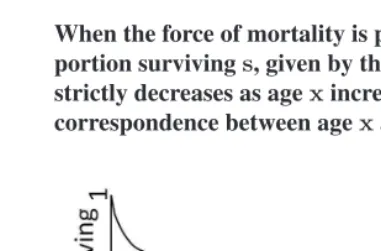
The life table`(x), constant in time, with continuous agex, is the proportion of a cohort (whether a birth cohort or a synthetic period cohort) that survives to agexor longer. In probabilistic terms,`(x)is one minus the cumulative distribution function of length of lifex. The maximum possible ageω may be finite or infinite. Ifω = ∞, then some individuals may live longer than any finite bound. By definition,`(0) = 1and`(ω) = 0. Assume`(x)is a continuous, differentiable function ofx,0 ≤ x≤ω, and assume life expectancy at age 0 is finite. The age-specific force of mortality at agexis, by definition,
(1) µ(x) =− 1
`(x)
d`(x)
dx .
Assumeµ(x) > 0 for all0 ≤ x ≤ ω. The life table `(x)is strictly decreasing from
`(0) = 1to`(ω) = 0so there is a one-to-one correspondence between agexin[0, ω]and the proportionsin[0,1]of the cohort that survives to agexor longer. One direction of this correspondence is given by the life table functions=`(x)(illustrated schematically in Figure 1 and for the United States population in 2004 in Figure 3A).
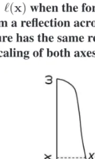
There appears to be no standard demographic term for the inverse function that maps the proportion surviving s, 0 ≤ s ≤ 1, to the corresponding agex, so I propose to call it the age functiona(illustrated schematically in Figure 2 and for the United States population in 2004 in Figure 3D). In words, the agea(s)at which the fractionsof the birth cohort survives is the agexat which the life table function`(x)iss. By definition, under the assumptionµ(x) >0for all0 ≤ x ≤ω,a(s) = xif and only if`(x) = s. Equivalently, by definition, for every s in0 ≤ s ≤ 1 and every xin0 ≤ x ≤ ω,
a(`(x)) =xand`(a(s)) =s. We definea(1/2)as the median life length, that is, the age by which half the cohort has died.
Figure 2: The functionx=a(s)that expresses the agexat which a fraction
sof a birth cohort survives is the inverse of the life table function
s=`(x)when the force of mortality is positive at every age. Apart from a reflection across the diagonal linex=s, the curve in this figure has the same relative shape as the curve in Figure 1 but the rescaling of both axes makes the two curves look different.
For everysin0 ≤ s≤1, we define the survival-specific force of mortalityλ(s)in terms of the age-specific force of mortalityµ(x)in (1) in three equivalent ways:
(2) λ(s) =µ(x) if s=`(x); or λ(s) =µ(a(s)); or λ(`(x)) =µ(x).
survival-specific force of mortalityλis0≤s≤1. We give below an explicit formula (9) for the survival-specific force of mortality at surviving proportions. This formula is analogous to (1) for the age-specific force of mortality.
The complete expectation of life at age x, e(x), is the average number of years remaining to be lived by those who have attained agex:
(3) e(x) = 1
`(x)
y=Zω−x
y=x
(y−x)`(y)µ(y)dy.
Inserting the definition (1) in place ofµ(y)in (3) and integrating by parts gives
(4) e(x) = 1
`(x)
aZ=ω
a=x
`(a)da,
a standard formula for life expectancy at agex(Keyfitz 1968:6).
1.2 Relationships
It is well known that the age-specific force of mortalityµ(x)equals a constantK > 0 at every agexif and only if the life table is negative exponential with parameterK, i.e.,
`(x) = exp(−Kx). In this case, the expectation of life at agexis the reciprocal of the age-specific force of mortality:
(5) e(x) = 1
K.
From the definition (2) of the survival-specific force of mortality, it is evident that
λ(s) = K > 0 at every surviving proportionsif and only if the life table is negative exponential with parameter K. Thus K in (5) may be viewed as a constant force of mortality, both age-specific and survival-specific.
Generalizations (6) and (8) extend (5) when the survival-specific force of mortality is
notconstant. These generalizations seem to be new. A first generalization of (5) states that
(6) e(x) = 1
`(x)
s=Z`(x)
s=0
In words, the expectation of life at agexis the average reciprocal of the survival-specific force of mortality weighted by the life-table deathsdsafter age x. Whenλ(s) = K, (6) simplifies to (5) because
(7) 1
`(x)
s=Z`(x)
s=0
ds= 1.
One can entirely eliminate agex(years of life lived in the past) from life expectancy (average years of life to be lived in the future) by defining a survival-specific life expectancyE(s)(analogous to the survival-specific force of mortality defined above) as the life expectancy when the surviving proportion of the birth cohort iss. Thus by defini-tion,E(s) =e(x)ifs=`(x)and equivalentlyE(s) =e(a(s))andE(`(x)) =e(x).
A second generalization of (5) is to rewrite (6) as
(8) E(s) = 1
s
s0=s Z
s0=0
ds0 λ(s0).
Heres0 is the running variable fors. In words, the life expectancy when the surviving
fraction issis the death-weighted average of the reciprocal of the survival-specific force of mortality over each survival proportion smaller than s. The substantive difference between (6) and (8) is that agexappears as an argument on both sides of (6) and nowhere in (8). An illustration of (8) using United States data will be discussed in section 4. Appli-cations.
We also demonstrate survival-specific forms of the force of mortality:
(9) λ(s) =−1
s ds da =−
1
s
µ
da ds
¶−1
.
2. Proofs
Sincea(s)and`(x)are inverse functions, elementary calculus shows that
(10) d`
dx =
µ
da ds
¶−1 = ds
da
(11) ds= µ
da ds
¶−1
da.
Then, fors= `(x)and running variabless0 =l(x0)(and with the equalities numbered
for subsequent explanation), we have
E(s)=1 e(x)
2 = 1
`(x)
x0=ω Z
x0=x −1
µ(x0) d`(x0)
dx0 dx 0
3 = 1
s
s0=s Z
s0=0 +1
λ(s0)
µ
da ds0
¶−1
da
4 = 1
s
s0=s Z
s0=0
ds0 λ(s0).
(12)
Equality 1 in (12) holds by definition ofE. Equality 2 takes (4) and replaces the integrand
`(a)in (4) with the result of exchanging`(x)andµ(x)in (1). Equality 3 uses the defi-nitionss=`(x)andλ(s) =µ(x)from (2), changes the minus one to plus one because of the reversal in the direction of integration, and uses (10) to replace one derivative with another. Finally, equality 4 uses (11) to “cancel” the differentialsda. This proves (8), and using the definitions=`(x)gives (6).
Finally, (9) follows immediately from the definitions (1) and (2) and the fact (10).
3. History and related results
I believe I was the first to state a special case of (6) in my first problem set dated 4 October 1971 for an undergraduate course on mathematical population models which I introduced at Harvard University (Biology 150). Assuming`(0) = 1, I asked the students to prove that
(13) e(0) =
1 Z
l=0
The text for the course was Nathan Keyfitz’s then recentIntroduction to the Mathematics
of Population (1968). When Keyfitz began teaching at Harvard in the fall of 1972,
I showed him (13) to find out if he had seen it before. He had not. I believe Keyfitz subsequently published (13), but not (6) or (8), as an exercise in one of his books. I can-not find the citation. To my knowledge, (6) and (8) and (9) have appeared nowhere before and no proof of (6), (8) or (13) has been published previously. The inequality (14) below also seems to be new.
4. Applications
4.1 Lower bound inequality
The expression (6) fore(x)yields a new lower bound on life expectancy at agex. The reciprocal function that maps each positive real number xinto 1/x is strictly convex. Therefore, Jensen’s inequality for the average of a convex function applies to (6) and yields
(14) e(x) = 1
`(x)
l=Z`(x)
l=0
dl λ(l)≥
1
1
`(x)
l=R`(x)
l=0
λ(l)dl
= `(x)
l=R`(x)
l=0
λ(l)dl .
This inequality is strict unless all deaths occur at a single age, that is, unless the life table is rectangular (in which case the age-specific force of mortality is not positive at ages less thanω), or unless the age-specific force of mortality is constant at all ages, in which case the survival-specific force of mortality is also constant. In words, the expectation of life at agexis at least as large as (and, apart from a rectangular life table or a constant force of mortality, is greater than) the reciprocal of the average survival-specific force of mortality weighted by life-table deathsdlat surviving proportions less than`(x), that is, at ages abovex.
4.2 Lower bound in the exponential distribution
and the denominator of the right side is
(15) K
l=Z`(x)
l=0
dl=K `(x) =K exp(−Kx).
Thus the right side of (14) equals`(x)/(K `(x)) = 1/Kand equality holds in (14), as expected in the case of a constant force of mortality.
4.3 Discrete actuarial approximations
If we are given the life-table proportions`xsurviving at each exact agex, the life-table
probabilityqx of dying by age x+ 1 given survival to exact agex, and the
expecta-tion of lifeex at exact age x, then the estimation of a(s), λ(s), andE(s) for given
surviving proportionss requires only linear (or other) interpolation. For example, the Matlab commandinterp1(lx,x,s,‘spline’)uses piecewise cubic spline inter-polation to producea(s)from three arguments: the life table expressed as a vectorlx, a vectorxof ages, and a vectorsof proportions surviving. Similarly, Matlab command
interp1(lx,qx,s,‘spline’) estimates the survival-specific force of mortality
λ(s)and Matlab commandinterp1(lx,ex,s,‘spline’)estimates the survival-specific life expectancyE(s). Both spline and linear interpolation were tried and the results were very similar. Spline interpolation was preferred to linear interpolation be-cause spline interpolation was smoother and took advantage of information outside the local interval of age.
The ability to compute a(s), λ(s), andE(s)using existing actuarial methods plus interpolation is a double advantage. It requires little retooling of methods or software, and it sheds new light on, and raises fresh questions about, familiar data, as the following example is intended to show.
4.4 Example based on life tables of the United States in 2004
Arias (2007) tabulated`x,qx, andexfor exact ages0,1,2, . . . ,99, and a terminal
catch-all group 100 years or older, for the 2004 United States population and eight subpopula-tions. Figure 3 plots (A)`(x)≈ `x, (B)µ(x)≈qx, and (C)e(x) ≈ex, for exact ages
for argumentsssmaller than`99 would have required extrapolation rather than interpo-lation. Just as Arias’s estimates for the age group 100 years or older required additional assumptions, estimates fors < `99would have required additional assumptions.
Figure 3: United States population in 2004 showing (A) the life table`(x),
(B) the age-specific force of mortalityµ(x), and (C) the expectation of remaining lifee(x),
as functions of agex, based on Arias (2007:Table 1) and (D) the agea(s)at which the proportionssurvives, (E) the survival-specific force of mortalityλ(s), and (F) the expectation of remaining lifeE(s)
as functions of the surviving proportions.
and substantially across the entire range ofs. Finally, while the age-specific expecta-tion of life (Figure 3C) falls gradually, almost linearly, across the entire range of age, the survival-specific expectation of life Figure 3F) rises slowly untilsapproaches 1 and then rises quite sharply. Looked at another way, by movingsin a decreasing direction from right to left in Figure 3F, the greatest losses in expectation of remaining life occur when the first small fraction dies (at highs). Thereafter, assdecreases further, the decline in expectation of remaining life is much more gradual.
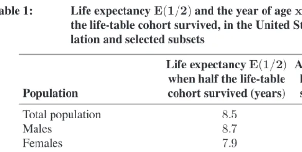
This perspective provides new ways to compare populations. To illustrate, Table 1 comparesE(1/2), the survival-specific life expectancy when half the cohort survives, as defined in (8), for the total population and eight subpopulations of the United States in 2004 (Figure 4), based on data of Arias (2007:Tables 1-9). For example, for the total population of the U.S. in 2004 (Arias 2007:Table 1), by exact age 81 the proportion sur-viving was 0.50987 with remaining life expectancy of 8.6 years and by exact age 82 the proportion surviving was 0.47940 with remaining life expectancy of 8.2 years. By linear interpolation I estimated a life expectancy of 8.4704 years when the proportion surviving was 0.5, and by spline interpolation I estimated a life expectancy of 8.4708, so I tabulated
E(1/2) = 8.5years. For simplicity in this illustration, the median life lengtha(1/2), that is, the age at which the proportion survivingsequaled1/2, was approximated by the whole number of years of life completed, that is, by the integer part ofa(1/2). Males’
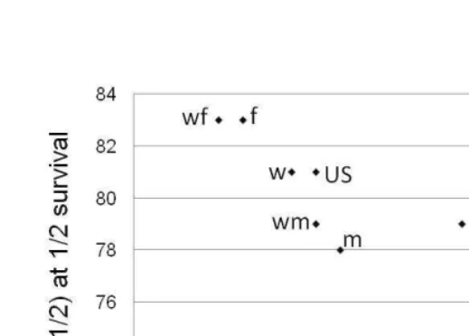
E(1/2)exceeded females’E(1/2)by 0.8 year but half the male cohort had died by age 78, five years younger than half the female cohort had died, by age 83. Similarly, the black population’sE(1/2)exceeded the white population’sE(1/2)by 2.3 years but half the black cohort had died by age 76, five years younger than half the white cohort died, at age 81. Of the subpopulations considered in Table 1, black males had the longest
E(1/2), 10.9 years, and the shortest median life length, reaching half survival youngest, at 72 years. White females had the shortestE(1/2), 7.7 years, and the longest median life length, 83 years, tied for oldest with all U.S. females. The younger half of a cohort died, that is, the shorter the median life length, the longer its life expectancy at that age.
This relationship is the opposite of the relationship expected from the simplest model, when the force of mortality is a constantK and the life table is negative exponential
`(x) = exp(−Kx). Thena(1/2) = ln(2)/K while the expectation of life (at any age or any surviving proportion) is1/K. Not surprisingly, the higher the force of mortality, the sooner half the cohort dies and the shorter the life expectancy. Both a(1/2) and
E(1/2)=e(a(1/2))are inversely proportional to the force of mortalityKand are directly proportional to one another in the family of negative exponential life tables with parameter
K, contrary to the observations of United States subpopulations.
pa-rameter or several papa-rameters (for example, the family of negative exponential life tables is indexed by the parameterK). One problem is to find necessary and sufficient condi-tions on the form of the life table and the values of the parameter(s) such thatE(s)and
a(s)are positively (or, negatively) associated as a parameter increases within some range. An empirical problem is to identify the demographic, economic, and cultural conditions under whichE(s)anda(s)are observed to be positively (or, negatively) associated, and to interpret these conditions in terms of the theoretical conditions.
Table 1: Life expectancyE(1/2)and the year of agextox+1in which half the life-table cohort survived, in the United States’ 2004 total popu-lation and selected subsets
Life expectancyE(1/2) Age when half the when half the life-table life-table cohort Population cohort survived (years) survived (years)
Total population 8.5 81-82
Males 8.7 78-79
Females 7.9 83-84
White population 8.3 81-82
White males 8.5 79-80
White females 7.7 83-84
Black population 10.6 76-77
Black males 10.9 72-73
Figure 4: Integer part of the age a at which half a cohort survived (vertical axis) as a function of the complete expectation of life at agea, for the United States total population and eight subpopulations, 2004, estimated by interpolation from data of Arias (2007)
US = total population, w = white, b = black, m = male, f = female
5. Acknowledgements
References
Arias, E. (2007). United States Life Tables, 2004.National Vital Statistics Reports56(9). Hyattsville, MD: National Center for Health Statistics. http://www.cdc.gov/ nchs/data/nvsr/nvsr56/nvsr56_09.pdf.