www.geosci-model-dev.net/7/1183/2014/ doi:10.5194/gmd-7-1183-2014
© Author(s) 2014. CC Attribution 3.0 License.
A technique for generating consistent ice sheet initial conditions for
coupled ice sheet/climate models
J. G. Fyke1, W. J. Sacks2, and W. H. Lipscomb1
1Group T-3, Los Alamos National Laboratory, Los Alamos, New Mexico, USA 2National Center for Atmospheric Research, Boulder, Colorado, USA
Correspondence to: J. G. Fyke ([email protected])
Received: 19 March 2013 – Published in Geosci. Model Dev. Discuss.: 15 April 2013 Revised: 7 April 2014 – Accepted: 23 April 2014 – Published: 23 June 2014
Abstract. A transient technique for generating ice sheet preindustrial initial conditions for long-term coupled ice sheet/climate model simulations is developed and demon-strated over the Greenland ice sheet using the Community Earth System Model (CESM). End-member paleoclimate simulations of the last glacial maximum, mid-Holocene op-timum and the preindustrial are combined using weighting provided by ice core data time series to derive continuous energy-balance-model-derived surface mass balance and sur-face temperature fields, which are subsequently used to force a long transient ice sheet model simulation of the last glacial cycle, ending at the preindustrial. The procedure accounts for the evolution of climate through the last glacial period and converges to a simulated preindustrial ice sheet that is geo-metrically and thermodynamically consistent with the prein-dustrial CESM state, yet contains a transient memory of past climate. The preindustrial state generated using this tech-nique notably improves upon the standard equilibrium spin-up technique, relative to observations and other model stud-ies, although in the demonstration we present here, large bi-ases remain due primarily to climate model forcing bibi-ases. Ultimately, the method we describe provides a clear template for generating initial conditions for ice sheets within a fully coupled climate model framework that allows for the effects of past climate history to be self-consistently included in long-term simulations of the fully coupled ice sheet/climate system.
1 Introduction
Ice sheets play an important role in regulating critical as-pects of the climate system such as sea level rise (Foster and Rohling, 2013), atmospheric circulation (Ridley et al., 2005) and ocean circulation (Weaver et al., 2003). Ice sheets can be considered coupled components of the climate sys-tem for several reasons. Ice sheet geometry is closely re-lated to climate via the surface mass balance (SMB) and sur-face temperature (Cuffey and Paterson, 2010): SMB defines where ice accumulates or melts and thus helps determines ice sheet geometry, while advection of surface temperature into ice sheets regulates the internal ice temperature distribu-tion and consequently ice rheology and basal sliding. Con-versely, ice sheet presence and evolution is a fundamental control on regional to hemispheric circulation patterns (e.g., Manabe and Broccoli, 1985), oceanic freshwater fluxes (e.g., Broecker, 1994) and regional climate behavior (e.g., Langen et al., 2012).
1184 J. G. Fyke et al.: Ice sheet spin-up for coupled models between all components of the climate model is required
before prognostic experiments can proceed. In traditional non-ice-sheet-enabled models, this consistency typically is acquired through spin-up to a stable equilibrium, with all coupling between components enabled. Ice sheets excluded, the slowest component of coupled models to equilibrate is usually the deep ocean, which reaches steady state after
∼103 years; this deep-ocean spin-up time ultimately deter-mines the coupled model spin-up simulation length. In typ-ical preindustrial coupled climate model spin-up exercises, the primary goal is to obtain a coupled model state in which all the physical and biogeochemical components (including the deep ocean) are in equilibrium with each other and with recent Holocene climate forcings (insolation, radiative gases, etc.) at the year 1850.
Inclusion of ice sheets in coupled models complicates this traditional ocean-limited preindustrial spin-up approach, for the basic reason that ice sheets reach quasi-equilibrium on average deep ice residence and lithospheric relaxation timescales, i.e., ∼104–105 years (i.e., 1–2 orders of mag-nitude slower than the ocean). This long equilibration time means that the present-day Greenland and Antarctic ice sheets (GrIS/AIS) are not in full equilibrium with preindus-trial (i.e., recent Holocene) climate. Rather, they contain a remnant thermal and dynamic memory of past glacial peri-ods that is reflected in present-day ice sheet conditions and potentially in long-term future ice sheet projections. Compu-tationally efficient stand-alone ice sheet model simulations forced with simple and highly parameterized climate repre-sentations driven by various paleoclimate time series are able to simulate the 104–105years necessary to capture this mem-ory (e.g., Huybrechts, 2002; Applegate et al., 2012). How-ever, an analogous synchronous fully coupled spin-up with a computationally expensive fully coupled ice sheet/climate model is simply not possible. Several approaches have been introduced to circumvent this computational barrier to gen-erating preindustrial coupled ice sheet/climate initial condi-tions. However, each method displays significant shortcom-ings:
– A computationally cheaper climate parameterization can be used to force an ice sheet model through one or more glacial periods. At some point, the resulting ice sheet could be inserted into the climate model (Vizcaíno et al., 2010). Shortcoming: this approach results in an artificial discontinuity in the ice dynamic response due to a step-function change in climate forcing that poten-tially affects future simulations.
– A positive-degree-day (PDD)-based SMB model could be used for past climates, with anomalies of model-simulated preindustrial temperature/precipitation condi-tions calculated using paleoclimate time series (Quiquet et al., 2013). Shortcoming: an analogous approach to scaling inputs to the SMB model is not feasible for more
physically consistent energy-balance-based SMB mod-els. Also, if a PDD model is used during spin-up, a dis-continuity will occur at the transition to the more consis-tent energy balance surface calculations within the cou-pled climate model framework.
– Asynchronous coupling could be used to accelerate the ice sheet and orbital forcings, relative to the rest of the climate. Shortcoming: abyssal-ocean- and ice-sheet-related limits to asynchronicity (Calov et al., 2009) still necessitate an extremely long climate simulation of 10 kyr or more to cover the entire last glacial cycle. – The ice sheet/climate model could be spun up under
constant preindustrial forcing (Fyke et al., 2011). Short-coming: while this approach may be valid for decadal-to-century-scale simulations (Seroussi et al., 2013), ne-glecting past climate history on preindustrial ice sheet conditions will affect the longer century-to-millennial-scale dynamic response of the ice sheets in coupled model simulations.
These issues point to a requirement for an alternate method for generating spun-up ice sheets that (a) is driven by uncor-rected conditions generated with integrated coupled climate model energy balance calculations; (b) has an internal mem-ory of the past glacial climate state (specifically as repre-sented by bias-uncorrected paleoclimate climate simulations) and (c) is self-consistent with the state of the climate-model-simulated preindustrial climate. These constraints must be satisfied so that the resulting ice sheet state can be “inserted” into a fully coupled framework as part of the suite of self-consistent component model initial conditions. In this study we describe and demonstrate one method for achieving this goal.
2 Models and methodology 2.1 Models
To develop a preindustrial ice sheet state that is compati-ble for use in a fully coupled modeling framework, we use a toolchain of models within the Community Earth System Model (CESM) framework. These include the fully coupled climate model CCSM4 (Gent et al., 2011), the stand-alone Community Land Model Version 4 (CLM; Oleson et al., 2010) and the Community Ice Sheet Model (CISM; Lip-scomb et al., 2013) within CESM1.1. We point the reader to the above references for detailed technical descriptions of CCSM4, CLM4 and CISM. Briefly, we summarize here that CISM is a shallow-ice-approximation thermomechani-cal ice sheet model on a 5 km resolution GrIS grid. It in-cludes a simple parameterization of basal sliding that de-pends on the presence of basal ice at the pressure melting point and a simple calving prescription in which all ice at floatation is instantaneously removed. SMB and surface tem-perature calculations over the GrIS are calculated using a full energy-balance-based SMB model at multiple vertical levels in CLM, the elevations of which are explicitly set to cover the full potential range of GrIS elevations. Importantly, SMB and surface temperatures are calculated at each time step in a full(x, y, z)matrix that includes locations where the GrIS surface does not exist. This feature is critical in the context of the ice sheet spin-up procedure described below, because it allows SMB and surface temperature values to be easily and directly interpolated to the evolving GrIS ice topography. This avoids complexities related to generating SMB lapse rates (Helsen et al., 2012) since it allows vertically interpo-lated climate-model-derived SMB values to be used directly during the ice sheet model simulation.
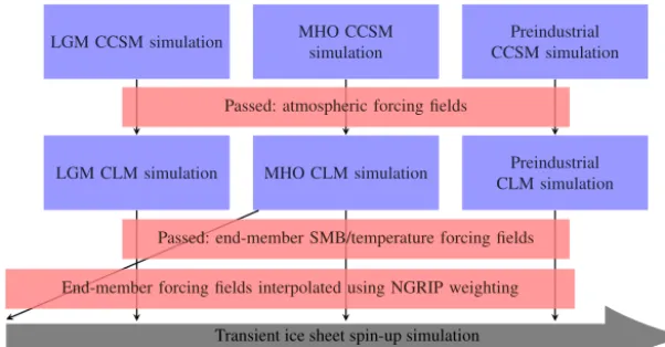
The ice sheet spin-up technique described here using CCSM4, CLM and CISM simulations can be briefly stated as follows: the coupled CCSM4 climate model was used to sim-ulate last glacial maximum (LGM), mid-Holocene optimum (MHO) and preindustrial climate states. Using output from these simulations, a corresponding set of CLM land surface model simulations were carried out to generate SMB and sur-face temperatures over Greenland for LGM, MHO and prein-dustrial climates. Composite SMB and surface temperatures at times between these “end-member” climate states were then calculated using weighting based on the North Green-land Ice Core Project (NGRIP) ice coreδO18 record (Wolff et al., 2010). This series of forcing fields is finally down-scaled via interpolation to the ice sheet model topography to drive a long CISM ice sheet model simulation. This process is described in more detail below and detailed graphically in Fig. 1.
2.2 End-member climate SMB and temperature generation
Previously, Brady et al. (2013) generated fully coupled equilibrium climate states for the LGM and MHO using the CCSM4. This same model configuration was also inte-grated to equilibrium under preindustrial conditions (Lan-drum et al., 2012). These “simulations of opportunity” pro-vided us with end-member climate states to use in testing our spin-up procedure. Unlike more recent versions of the CESM, the version of CLM within these CCSM4 simulations did not include in-line SMB calculations. However, included in the output of each of these large-scale simulations were the necessary atmospheric fields required to drive an updated version of CLM, which includes calculations for generat-ing in-line SMB and surface temperature values at multi-ple elevation levels over Greenland. We thus used the final 30 years of output from the previously performed coupled climate model simulations of the LGM, MHO and preindus-trial periods as looped input forcing for three corresponding CLM4 simulations, which were integrated for 200 years each to equilibrium and from which the final 30 years of equilib-rium LGM, MHO and preindustrial SMB and surface tem-perature matrices were obtained at multiple vertical levels on the coarse CLM4 grid.
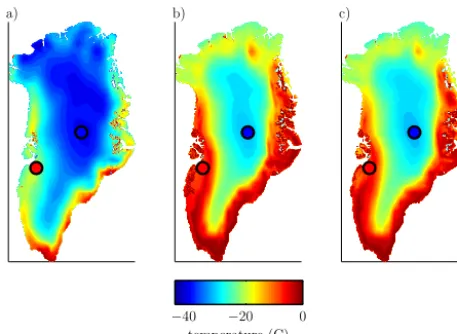
These 30 year equilibrium SMB and surface temperature climatologies formed the basis from which the continuous forcing for the long transient ice sheet model spin was gener-ated (Sect. 2.3). The downscaled end-member LGM, MHO and preindustrial SMB and surface temperature fields based on these climatologies are shown in Figs. 2 and 3. To ensure a sufficient spin-up length, the simulation was initialized at the end of the last interglacial (LIG). However, an appropri-ate fully coupled CESM LIG simulation was not available. We thus assumed the MHO to be the best approximation for the LIG and copied this forcing state for use as an idealized initial end-member LIG SMB forcing. The bias in ice sheet evolution resulting from using MHO forcing as a proxy for LIG climate conditions had little effect on the final preindus-trial ice sheet state (which was the primary target of the sim-ulation) since the memory of this forcing was swept from the system during the cold glacial period (Sect. 3). Full 30-year climatologies of SMB and surface temperature were used to ensure that both the mean climatology and any non-zero im-pacts on ice sheet evolution due to interannual SMB vari-ability about the mean (Pritchard et al., 2008) were properly captured.
2.3 Continuous ice sheet model boundary condition generation
1186 J. G. Fyke et al.: Ice sheet spin-up for coupled models
Discussion
P
ap
er
|
Dis
cussion
P
ap
er
|
Discussion
P
ap
e
r
|
Discussion
P
ap
er
|
MHO CCSM simulation
LGM CCSM simulation Preindustrial
CCSM simulation
MHO CLM simulation
LGM CLM simulation Preindustrial
CLM simulation Passed: atmospheric forcing fields
Passed: end-member SMB/temperature forcing fields
End-member forcing fields interpolated using NGRIP weighting
Transient ice sheet spin-up simulation
Fig. 1.Work flow for the procedure described in this study. Atmospheric output from global model simu-lations is used to drive land-surface model simusimu-lations. These simusimu-lations generate surface mass balance fields necessary to force the ice sheet model simulation (after ice core data-weighted interpolation be-tween bounding end-member SMB and temperature fields, and interpolation to the ice sheet geometry). Blue boxes: End-member simulations; red boxes: fields passed from one simulation to the next; grey arrow: final ice sheet simulation. Note use of MHO climate as a proxy for the LIG (diagonal arrow).
28
Figure 1. Work flow for the procedure described in this study. Atmospheric output from global model simulations is used to drive land-surface model simulations. These simulations generate the surface mass balance fields necessary to force the ice sheet model simulation (after ice core data-weighted interpolation between bounding end-member SMB and temperature fields and interpolation to the ice sheet geometry). Blue boxes: end-member simulations; red boxes: fields passed from one simulation to the next; grey arrow: final ice sheet simulation. Note use of MHO climate as a proxy for the LIG (diagonal arrow).
was done using a technique adopted and modified from stand-alone ice sheet model spin-up approaches. First, rep-resentative LGM, MHO(/LIG) and preindustrial δO18 val-ues were calculated by averaging the 600 years of NGRIP values bounding each time period from the NGRIP δO18 record (Wolff et al., 2010) (for the preindustrial climate, NGRIP values corresponding to the interval 1250–1850 were used). The 600-year averaging avoided aliasing of LGM, MHO and preindustrial end-member climate NGRIP val-ues due to centennial-scale variability in the NGRIP record. The δO18 record was then thresholded slightly to account for the fact that time periods represented by the climate model end-member simulations did not fall exactly on maxi-mum/minimum MHO/LGM NGRIP values. This avoided ar-tificial extrapolation of SMB values beyond the cold/warm LGM/MHO cases, which would have potentially introduced non-realistic extrapolated SMB values such as negative SMB at the summit during the LGM and too-high accumulation during the LIG/MHO. The practical impact of this thresh-olding was to set SMB values of cold pre-LGM glacial peri-ods between interstadials to slightly higher model-simulated LGM values, despite suggestions from the isotopic record that these periods were actually slightly more extreme.
The resulting thresholded NGRIP δO18 record was then used to guide the time interpolation between the end-member SMB and surface temperature matrices for every time step and(x, y, z)location between the LIG and the preindustrial climates. Climate was assumed to vary in 600-year steps. For each 600-year period, a weight between bracketing climate end-members was determined. A 30-year SMB/surface tem-perature climatology was then constructed for this interval by a linear interpolation of SMB and temperature values from the appropriate years of the bounding end-member climates
(Figs. 2 and 3):
wt−1=
δ18OEM+1−δ
18O CC
δ18O
EM+1−δ18OEM−1
, (1)
wt+1=1−wt−1, (2)
SMB(x, y, z)yrCC=1:30= [SMB(x, y, z)yrEM=1:30
−1 wt−1] + [SMB(x, y, z)yrEM=1:30
+1 wt+1], (3)
T (x, y, z)yrCC=1:30= [T (x, y, z)yrEM=1:30
−1 wt−1] + [T (x, y, z)yrEM=+1:30
1 wt+1], (4)
where EM−1and EM+1represent bounding end-member
cli-mates for a particular mid-run climate period CC and CC in-creases by 1 for every 600-year period (for example, for a period CC in middle of the last glacial period EM−1=LIG
and EM+1=LGM). The interpolated 30-year SMB/surface
c)
temperature (C) b)
a)
−40 −20 0
1
Figure 2. 30-year climatological annual average surface tempera-ture fields for the LGM (a), MHO (b) and preindustrial (c) end-member climate states. Blue/red circles: location of the sum-mit/margin temperature time series presented in Fig. 4.
at 122 ka with a present-day geometry based on a modified version of that presented in Bamber et al. (2001). Initial in-ternal temperature profiles trended linearly from the CESM-simulated preindustrial surface temperature 2 degrees Cel-cius below the location-specific pressure-dependent melting point. From this initial condition the transient temperature and SMB forcings drove ice sheet model evolution.
The ice sheet model had previously undergone a perturbed-physics analysis to determine a set of ice sheet pa-rameters that corresponded to an optimal steady-state GrIS geometry under constant preindustrial climate (Lipscomb et al., 2013). We adopted these parameters for the present study, despite their being generated using an ensemble of equilibrium simulations. A full implementation of the spin-up technique (demonstrated here with one simulation) will ultimately involve a large, computationally intensive ensem-ble of transient spin-up simulations and subsequent selec-tion of optimal ensemble members (e.g., Applegate et al., 2012). We chose not to undertake this effort for the present study, which is meant primarily as a demonstration of the transient spin-up procedure and not as a full optimization ex-ercise to identify optimal ice sheet parameter combinations. Finally, compared to the simulations presented in Lipscomb et al. (2013), some additional structural model changes were present: the number of elevation levels in CLM was increased to 36, the maximum snow depth in CLM was increased to 5 m water equivalent (w.e.), and a sub-grid snow-rain parti-tioning routine to segregate incoming precipitation based on downscaled surface temperature was included.
3 Results
To demonstrate the procedure outlined above, a full LIG-to-preindustrial transient ice sheet simulation was performed.
c)
SMB (m WE/yr) b)
a)
−3 −2 −1 0 1
1
Figure 3. 30-year climatological SMB fields for the LGM (a), MHO (b) and preindustrial (c) end-member climate states. Blue/red circles: location of the summit/margin SMB time series presented in Fig. 4.
In the following section we describe important aspects of this simulation, with a particular focus on trends in surface conditions during the simulation and differences in the final preindustrial state relative to a spin-up simulation driven with constant preindustrial forcing. We place emphasis on evalu-ation of trends in surface SMB and surface temperature and comparison to the equilibrium spin-up simulation rather than the absolute surface conditions themselves, which are a func-tion of the broader climate model state. This is motivated by our aim not to validate the overlying climate model forcing (which is a large and ongoing task that is subject to change as CESM is developed further) but rather to verify that the spin-up procedure produces qualitatively correct trends in surface conditions and improves in a relative sense over an equilib-rium spin-up approach. In addition, it is important to note that the CCSM4 climate simulations used here were simu-lations of opportunity, in the sense that they were the only fully coupled and equilibrated CCSM4 or CESM paleocli-mate simulations available. While they provided broad forc-ing reflective of LGM, MHO and preindustrial time periods, they were never initially intended to provide GrIS surface conditions (or formally evaluated over the GrIS). Thus, we emphasize that these climate model simulations were used, in the context of this study, only to help demonstrate an ap-plication of the transient spin-up method template rather than specifically generate an accurate and data-constrained recon-struction of GrIS behavior over the last glacial cycle. 3.1 Evolution of surface forcing conditions
1188 J. G. Fyke et al.: Ice sheet spin-up for coupled models
c) b) a)
time (kyr BP)
to ta l S M B (G t/ y r) te m p e ra tu re (C ) S M B (m / y r w .e .) te m p e ra tu re (C ) S M B (m / y r w .e .)
−100 −90 −80 −70 −60 −50 −40 −30 −20 −10 −100 −90 −80 −70 −60 −50 −40 −30 −20 −10 −100 −90 −80 −70 −60 −50 −40 −30 −20 −10 −100 −90 −80 −70 −60 −50 −40 −30 −20 −10 −100 −90 −80 −70 −60 −50 −40 −30 −20 −10 200 400 600 800 −40 −35 −30 0.15 0.2 −20 −15 −10 −1 0 1
Figure 4. Time series of integrated GrIS SMB (a). Marginal/summit specific SMB (b): margin location is blue and the summit location is green; the vertical axes scaling is different for the two time se-ries to highlight the anticorrelated relationship between the two. Marginal/summit surface temperature (c): margin location is blue and the summit location is green.
and a representative western ablation zone location (the loca-tions of these sample points are highlighted in Figs. 2 and 3). A comparison of SMB and surface temperature time series at these two locations highlights important strengths of the spin-up technique. Near-surface temperature trends on the margin are similar to interior trends and, as expected, temper-atures in both regions decrease during glacial periods. The temperature at the summit ranges from −30◦C to−40◦C: the maximum simulated temperature compares well with that reconstructed from the Greenland Ice Core Project (GRIP) temperature profile (Dahl-Jensen et al., 1998), but the min-imum simulated LGM temperature is significantly warmer. This is partly due to the fact that thresholding of the NGRIP
δO18 record described in Sect. 2 thresholds cold pre-LGM stadial temperatures, which the CESM LGM simulation does not represent. Surface temperatures at the marginal location are always warmer than those in the interior, ranging from
−7◦C to−21◦C.
In contrast to temperature trends, SMB trends in the in-terior are generally anticorrelated to trends on the margin. During a glacial state, summit SMB decreases from over 0.2 m w.e. yr−1to 0.11 m w.e. yr−1, in agreement with accu-mulation rates derived from the GRIP ice core (Dahl-Jensen et al., 1993). On the other hand, margin SMB increases from
−2 m w.e. yr−1to 0.05 m w.e. yr−1. The opposite response of the two locations results from a lack of ablation in the in-terior and decreased atmospheric moisture transport in cold climates. At the summit, since no ablation occurs at any time,
b) a) -5 -5 -5 -10 -10 -10 -15 -15 -15 -20 -20 -20 -25 -25 -25 -30 -30 -30 -35 -35 -35 -35 -35 -35 b a sa l T (C )
time (kyr BP)
d e p th b e lo w su rf a ce (m )
−100 −90 −80 −70 −60 −50 −40 −30 −20 −10 −3.5
−3 −2.5 −3000 −2500 −2000 −1500 −1000 −500 0 1
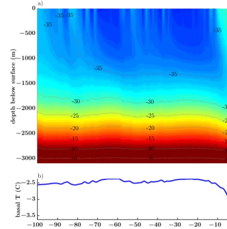
Figure 5. (a) Temperature evolution through time of the simulated ice column at the location of the observed GIS summit; (b) basal temperature evolution.
the simulated decrease in precipitation during glacial peri-ods causes a decrease in SMB. This glacial decrease is due to a combination of decreased moisture availability from in-creased sea ice cover, dein-creased marine boundary layer evap-orative potential and decreased moisture-carrying capacity of cold air. In contrast, marginal ablation zone SMB becomes much less negative, and even slightly positive, during glacial periods due to a reduction in ablation during glacial peri-ods. Qualitative reproduction of the interior and margin SMB trends in glacial climates thus serves as a validation of the ba-sic climate model phyba-sics.
3.2 Evolution of ice sheet temperature
c) b) a)
time (yr BP)
e
le
v
a
ti
o
n
(m
a
sl
)
a
re
a
(k
m
2)
v
o
lu
m
e
(k
m
3)
−100 −90 −80 −70 −60 −50 −40 −30 −20 −10
−100 −90 −80 −70 −60 −50 −40 −30 −20 −10
−100 −90 −80 −70 −60 −50 −40 −30 −20 −10
×106 ×106
2900 3000 3100 3200 3300 2.05 2.1 2.15 2.2 2.25 3.3 3.4 3.5 3.6 3.7
1
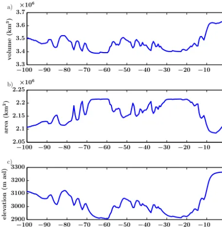
Figure 6. Time series of total GIS volume (a), GIS area (b) and GIS summit elevation (c).
warmer than ice at mid-depths. This inversion decreases with time as the cold glacial signal advects marginwards and the transition from the MHO to the preindustrial climate cools the upper ice. However, cold mid-depth ice remains at the end of the transient spin-up simulation, in good agreement with the temperature profile obtained at the GRIP site (Greenland Ice-Core Project Members, 1993).
The evolution and final state of the basal temperature field is also important, since the distribution of basal ice tem-peratures at the pressure melting point determines where basal sliding may potentially occur. Basal temperature shows a very damped response to surface temperatures changes. Nonetheless, the extended cold signal of the LGM is suffi-cient to penetrate to the bottom of the ice sheet in the tran-sient spin-up simulation and actively depresses the basal tem-peratures at the preindustrial period (Fig. 5b). This delayed present-day cooling response to LGM conditions occurs at the same time that shallower regions of the central ice sheet display warming, highlighting one aspect of the multiple re-sponse timescales inherent in the GrIS.
3.3 Evolution of ice sheet geometry
The simulated CISM ice sheet geometry evolves through the simulation, in response to the transient SMB and surface temperature forcing. Ice summit elevation primarily changes in response to the interior accumulation trends. During the LGM glacial period, the strong decrease in precipitation in the interior is reflected by a corresponding 100–200 m drop in summit elevation compared to the MHO/preindustrial ele-vation (Fig. 6). The eleele-vation drop at the LGM relative to the
MHO/preindustrial elevation is consistent with previous es-timates of summit elevation changes based on modeling esti-mates that assume little margin migration (Cuffey and Clow, 1997), which is the case in the transient spin-up simulation. At the same time, margins of the LGM ice sheet thicken due to decreased ablation. The net effect of these two pro-cesses is a decrease in simulated LGM ice volume relative to MHO/preindustrial ice volumes, since the decrease in inte-rior ice volume outweighs the increase in marginal thickness. Post-deglaciation, the summit elevation increases then re-mains relatively constant between the MHO and preindus-trial states. This behavior is consistent with previous mod-eling, but not with data-based estimates which suggest sum-mit thinning between the MHO and the preindustrial (Vinther et al., 2009). The overall increase in post-glacial summit ele-vation is reflected by an interior ice volume increase while at the same time anomalously low MHO-preindustrial ablation around the margins results in (a) little margin retreat, (b) net integrated SMB which at the end of the simulation is sig-nificantly (∼60 %) higher than the historical SMB (Ettema et al., 2009) and (c) anomalously high marginal and total ice volume at the preindustrial (Fig. 6). Over the final 4200 years of the simulation, the ice sheet gains ice volume at a modest rate of 9 km3yr−1, in rough agreement with the estimate of 20 km3yr−1made by Huybrechts (1994). The spatial pattern of surface elevation change dH /dt also agrees qualitatively with Huybrechts (1994), in that late Holocene mass gain is concentrated at the margins of the ice sheet, particularly the southwest.
1190 J. G. Fyke et al.: Ice sheet spin-up for coupled models
el
ev
at
io
n
ab
ov
e
se
a
le
ve
l
(m
)
a)
distance (km)
b)
1
0 0 0
0 0
0
0
0
0 0
0 0
0
0 0
0
0
0
-1
-1
-1 -1
-1
-1
-2
-2 -2
-2
-2 -3
-3 -3
-3
-3 -4
-5
200 400 600 800 1000 1200 −40 −20 0 0
500 1000 1500 2000 2500 3000 3500
0 500 1000 1500 2000 2500 3000 3500
1
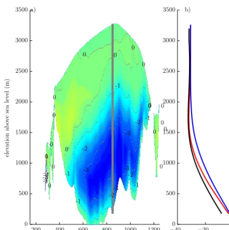
Figure 7. (a) Difference in final preindustrial temperature across the central ice sheet between transient and equilibrium spin-up simula-tions (blue: transient simulation is colder); (b) comparison of ver-tical temperature profiles at observed summit location to the GRIP temperature profile. Red: transient up; blue: equilibrium spin-up; black: GRIP temperature profile.
3.4 Comparison of transient spin-up to equilibrium spin-up at the preindustrial
A comparison of the final preindustrial state of the transient up simulation to the final state of the equilibrium spin-up simulation provides a robust benchmark for assessing the impact of climate history on the spin-up procedure. The fun-damental utility of a transient spin-up in improving preindus-trial ice sheet states has been previously well demonstrated (e.g., Huybrechts, 1994). Here, we identify improvements of the transient spin-up relative to the equilibrium spin-up sim-ply to show that the transient spin-up method we have devel-oped performs as expected, despite the imposed constraints which ensure consistency when the final state is used as an initial condition within a coupled climate model framework. Figure 7a plots the difference in preindustrial internal tem-peratures between the transient and equilibrium spin-ups, across the same cross section that contains the summit col-umn plotted in Fig. 5. The difference in temperature is small (less than 1◦C) in the upper ice column but increases to
al-most 5◦C in the deep interior. Figure 7b plots the observed GRIP temperature profile (Greenland Ice-Core Project Mem-bers, 1993) against the equivalent preindustrial transient and equilibrium spin-up profiles. The transient spin-up does a significantly better job at matching the GRIP temperature profile, confirming the ability of the spin-up procedure to better reflect past ice history in the final ice sheet internal
temperature (C) b)
temperature (C) a)
−8 −6 −4 −2 0
−8 −6 −4 −2 0
1
Figure 8. Preindustrial basal temperatures for both transient (a) and equilibrium spin-up (b) simulations.
state. The temperature at the base of the GRIP core location is significantly warmer than observed in both the transient and equilibrium spin-up simulations (though slightly less so in the case of the transient spin-up): this is perhaps due to too high a prescribed geothermal heat flux in this location rela-tive to the actual flux and/or due to spatial biases in the sim-ulated temperature distribution (highlighted by the fact that a∼40 km shift in the location of the simulated GRIP perature profile would provide a much better basal ice tem-perature comparison). Regardless, the presence of this bias in both simulations indicates that the issue is related to other aspects of model design and not specifically to the spin-up technique.
c) b)
a)
elevation (masl)
0 2000
1
Figure 9. Surface heights for transient spin-up simulation preindus-trial state (a), equilibrium spin-up simulation preinduspreindus-trial state (b) and observed geometry (c). Both model simulations clearly overes-timate ice thickness and resulting surface height around the margins.
minor impact on overall evolution. However, were a higher-order ice sheet model with greater sliding-derived transport to be used instead, the change in the extent of basal sliding due to spin-up technique could play a more important role in determining both the preindustrial ice sheet state and future evolution of the model.
Final preindustrial surface elevations for the two spin-ups are shown in Fig. 9a and b, the observed GrIS surface eleva-tion is shown in Fig. 9c, and the difference in the simulated surface elevations is displayed in Fig. 10. As noted previ-ously, the model generates too much marginal ice, regardless of the spin-up procedure. Thus, decreases in marginal ice volume represent an improvement in model performance. To this end, the transient spin-up simulation displays decreases in ice thickness of up to 500 m in the northern ice sheet rel-ative to the equilibrium spin-up simulation (Fig. 10): this difference likely arises from decreased accumulation during the LGM, followed by the warm period of the MHO during which simulated near-coastal ablation was somewhat higher than during the preindustrial. The ice sheet interior is slightly higher in the transient spin-up case compared the equilib-rium spin-up case, likely due to the influence of decreased basal sliding resulting from colder basal temperatures. Both of these effects nudge the transiently spun-up preindustrial state closer to the observed ice sheet geometry, compared to the equilibrium spin-up simulation.
4 Discussion
In this work we have described and demonstrated a tech-nique for generating ice sheet initial conditions for use in future fully coupled climate model simulations that are geo-metrically and thermodynamically consistent with the prein-dustrial climate model state yet contain a transient memory
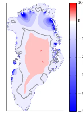
height difference (m)−500
−400
−300
−200
−100
0 100
1
Figure 10. Difference in surface topography between transient and equilibrium simulation preindustrial states: blue colors indicate that the transient spin-up state is lower, while red colors indicate that the transient spin-up state is higher. The thick grey line is the zero-contour.
1192 J. G. Fyke et al.: Ice sheet spin-up for coupled models SMB fields prior to use as ice sheet model boundary
condi-tions, as this would also make the resulting ice sheet state inconsistent with the climate-model-derived forcing. Finally, we cannot (within the scope of this method’s description) tune CESM to provide more realistic SMB fields in the same way that a highly parameterized representation of ice sheet climate forcing can be tuned. This is because CESM is a full-complexity climate model that is ultimately forced by plan-etary boundary conditions, and tuning such a model practi-cally is not a simple “order 1” parametric sensitivity study but rather an ongoing CESM community effort.
The constraints we impose in our spin-up result in a sig-nificant overestimate of the final GrIS volume, largely due to SMB overestimates from the end-member CESM simula-tions. However, the goal of the exercise is to demonstrate the ability to generate an ice sheet state that is consistent with cli-mate model forcing, not to generate an accurate GrIS recon-struction through the last glacial cycle. Within this context, the overestimated volume does not preclude the success of the method. Instead, it points to clear routes to improvement in the overlying CLM and CESM model that are the target of ongoing global climate model tuning exercises. More gener-ally, it is notable that all the other the non-land-ice compo-nents of the CESM also display significant historical biases (e.g., de Boer et al., 2012; Lawrence et al., 2012; Bates et al., 2012; Kopparla et al., 2013); the ice volume overestimate we obtain is directly analogous to these biases and must be re-duced though comprehensive global coupled model improve-ment.
Inverse procedures (e.g., Arthern and Gudmundsson, 2010; Price et al., 2011; Gillet-Chaulet et al., 2012) have been used recently to calculate basal drag coefficient fields such that the difference between simulated and observed ve-locities is minimized. Inverse methods are primarily aimed at generating initial conditions for short-term ice sheet forecasts which (like weather forecasts) ideally require initial states very close to those which are observed. However, it is not clear that such methods are feasible alternatives to the ap-proach described here for century-to-millennia scale simu-lations using fully coupled ice sheet/climate models. Since coupled models are in no way constrained by observations during run-time, an equilibrated coupled model representa-tion of the preindustrial will almost invariably display (hope-fully small) biases compared to observations, including bi-ases in ice sheet state: this is the trade-off for fully coupled system consistency. Conversely, an ice sheet state that is in force balance and reproduces observed velocities will dis-play negligible biases compared to observations but will very likely be inconsistent with any model-derived climate. Thus, if an ice sheet initialized by an observationally constrained inverse method were to be inserted into the CESM or another climate model, an initialization shock would occur as the ice sheet velocities, temperature distribution and geometry read-justed to the new fully coupled surface forcings. It could be possible to derive a cost function to integrate climate model
surface forcings into the inversion procedure, such that the optimal inverted basal drag coefficient field results in an ice sheet that respects both balance velocities and modeled sur-face conditions such as SMB and temperature (Price et al., 2011). However, additional issues could arise. For example, any climate model biases that are reflected in the simulated SMB would not be removed but simply transferred to the ice sheet model basal traction coefficient field. Perhaps more critically, any ice sheet model within a coupled model must be allowed to incept or expand into ice-free regions, but it is not clear how inversion techniques would account for ice ex-pansion where no ice velocity exists in current observations. The ability to expand to currently ice-free regions is critical for simulated preindustrial climate consistency and certainly for coupled simulations of colder periods such as the LGM.
Several recent studies have utilized large ensembles of ice sheet simulations to optimize important ice sheet model pa-rameters (Stone et al., 2010; Applegate et al., 2012; Lip-scomb et al., 2013). The impact of a transient spin-up on optimal ice sheet parameters could manifest itself in several ways. A transient spin-up results in colder interior tempera-tures in much of the interior of the ice sheet, particularly in deeper ice where deformational flow is strongest. Thus, the optimal ice sheet parameter set should tend to have a higher flow enhancement factor compared to an equilibrium spin-up if this is one free parameter in the optimization. Lower basal temperatures should shrink the regions where basal sliding occurs. To compensate, optimal basal sliding coef-ficients should generally be higher in sliding regions for the case where transient spin-ups are used.
to document and demonstrate the spin-up approach itself, us-ing presently available coupled simulations. To that end, gen-eral model behavior such as the generation of spatially vari-able SMB trends of opposite sign, the residual LGM internal ice temperature signal that matches observations, and the in-crease in summit elevation between LGM and preindustrial suggest that the spin-up technique is reasonable and can be used to generate preindustrial ice sheet initial conditions as part of the suite of initial conditions for fully coupled CESM simulations of future climate change.
Testing the long-term impact of the climate-consistent restart that we present here requires simulations past the year 2100, since prior to this time, the majority of the ice re-sponse is due to atmospheric and oceanic boundary condi-tion changes and not to the internal climate history of the ice (Seroussi et al., 2013). Only after several hundred years do the effects of ice dynamics begin to play a major role in determining the ice sheet evolution (Ridley et al., 2005). However, to date, CESM simulations including SMB have only extended to the year 2100 and, in addition, have not contained a full representation of two-way ice sheet/climate coupling. This coupling is required past the year 2100 due to the increasing strength of ice sheet/climate feedbacks (Viz-caíno et al., 2010). Completion of the full ice sheet/climate model CESM-CISM (Fyke et al., 2014b) will allow for a full analysis of the consistency of the spun-up ice sheet state within the fully coupled framework and a robust analysis of the role of ice sheet spin-up procedure in determining multi-century (post-2100) GrIS evolution trends. This work will be reported in upcoming studies; here we focus on detailing the methodology behind the spin-up technique we will use in these coupled simulations.
5 Conclusions
We have described and demonstrated a new procedure for generating a simulated preindustrial ice sheet state for use in fully coupled ice sheet/climate models. The procedure gener-ates an ice sheet state that is consistent with simulated prein-dustrial climate forcing but also contains a consistent thermo-dynamic memory of climate-model-simulated paleoclimatic conditions. As a result, the effect of past climate on future ice sheet evolution is captured while non-physical trends in the ice sheet component of future ice sheet/climate simulations are avoided. This capability allows for the creation of consis-tent ice sheet/climate conditions that can be used as part of the set of initial conditions for coupled model simulations of future ice sheet and sea level change.
The technique was developed within the CESM frame-work. It uses ice core data to guide interpolation of surface mass balance and temperature fields generated from CLM simulations (driven by forcing from previous fully coupled CESM simulations) in order to generate the time-continuous forcing required for long ice sheet spin-up simulations.
Unique to this approach is the use of matrices of surface mass balance and temperature fields generated using an un-bias-corrected energy balance model instead of a simpler positive-degree-day approach. The procedure results in a preindustrial ice sheet geometry and temperature distribution that fully re-flects both simulated preindustrial and earlier paleoclimate climate states yet avoids artificial climate forcing discon-tinuities, which is a necessary precondition for consistent fully coupled simulations of future coupled ice sheet/climate change.
We demonstrated the feasibility of the procedure for the Greenland ice sheet by carrying out a full 122 000 year sim-ulation from the LIG to the preindustrial period. The ice sheet simulation displayed qualitatively correct surface mass balance, vertical summit migration and internal temperature evolution trends. At the preindustrial, a residual LGM ther-mal signature was present in the simulated ice sheet and important improvements were apparent over a correspond-ing spin-up uscorrespond-ing constant preindustrial forccorrespond-ing. Internal and basal ice temperatures were up to 5◦C cooler compared to a spin-up forced with constant preindustrial conditions and ice sheet thickness was improved in places by up to 500 m compared to observed thicknesses. Excess ice thickness pri-marily due to climate model forcing biases remained around the margins, resulting in an overestimate of the preindustrial GrIS volume. However, this ice volume bias does not pre-clude the demonstrated ability of the spin-up procedure to generate an ice sheet state with a dynamic and thermody-namic memory of past climate that is consistent with the simulated preindustrial climate. Rather, it emphasizes that improvements to climate-side surface mass balance calcula-tions are important in order to produce a spun-up ice sheet state that better matches observations. Thus, we are confi-dent that the technique described here is a feasible approach for providing consistent ice sheet initial conditions within a fully coupled ice sheet/climate model framework.
Acknowledgements. The authors wish to acknowledge Bette
Otto-Bliesner and colleagues for providing CESM simulation output. Support was provided by the National Science Foundation through Award ANT-1103686 for William J. Sacks. Support for William H. Lipscomb was also provided by the Scientific Discovery through Advanced Computing (SciDAC) project funded by the US Department of Energy, Office of Science, Advanced Scientific Computing Research and Biological and Environmental Research (BER). Jeremy G. Fyke was supported by the Regional Arctic System Modeling project funded by BER and by the National Science Foundation Office of Polar Programs. The CESM project is supported by the National Science Foundation and the Office of Science (BER) of the US Department of Energy. NCAR is sponsored by the National Science Foundation.The simulations were carried out on the Yellowstone computing system (National Center for Atmospheric Research, Computational and Information Systems Laboratory, 2014).
1194 J. G. Fyke et al.: Ice sheet spin-up for coupled models References
Applegate, P. J., Kirchner, N., Stone, E. J., Keller, K., and Greve, R.: An assessment of key model parametric uncertainties in projec-tions of Greenland Ice Sheet behavior, The Cryosphere, 6, 589– 606, doi:10.5194/tc-6-589-2012, 2012.
Arthern, R. and Gudmundsson, G.: Initialization of ice-sheet fore-casts viewed as an inverse Robin problem, J. Glaciol., 56, 527– 533, 2010.
Bamber, J. L., Layberry, R. L., and Gogineni, S.: A new ice thick-ness and bed data set for the Greenland ice sheet 1: Measurement, data reduction, and errors, J. Geophys. Res., 106, 33773–33780, 2001.
Bates, S. C., Fox-Kemper, B., Jayne, S. R., Large, W. G., Stevenson, S., and Yeager, S. G.: Mean biases, variability, and trends in air– sea fluxes and sea surface temperature in the CCSM4, J. Climate, 25, 7781–7801, doi:10.1175/JCLI-D-11-00442.1, 2012. Brady, E., Otto-Bliesner, B., Kay, J., and Rosenbloom, N.:
Sensitiv-ity to glacial forcing in the CCSM4, J. Climate, 26, 1901–1925, doi:10.1175/JCLI-D-11-00416.1, 2013.
Broecker, W.: Massive iceberg discharges as triggers for global cli-mate change, Nature, 372, 421–424, 1994.
Calov, R., Ganopolski, A., Kubatzki, C., and Claussen, M.: Mech-anisms and time scales of glacial inception simulated with an Earth system model of intermediate complexity, Clim. Past, 5, 245–258, doi:10.5194/cp-5-245-2009, 2009.
Charbit, S., Ritz, C., and Ramstein, G.: Simulations of Northern Hemisphere ice-sheet retreat: sensitivity to physical mechanisms involved during the Last Deglaciation, Quaternary Sci. Rev., 21, 243–265, doi:10.1016/S0277-3791(01)00093-2, 2002.
Charbit, S., Ritz, C., Philippon, G., Peyaud, V., and Kageyama, M.: Numerical reconstructions of the Northern Hemisphere ice sheets through the last glacial-interglacial cycle, Clim. Past, 3, 15–37, doi:10.5194/cp-3-15-2007, 2007.
Cuffey, K. and Clow, G.: Temperature, accumulation, and ice sheet elevation in central Greenland through the last deglacial transition, J. Geophys. Res., 102, 26383–26396, doi:10.1029/96JC03981, 1997.
Cuffey, K. and Paterson, W.: The Physics of Glaciers, Elsevier, Am-sterdam, 2010.
Dahl-Jensen, D., Johnsen, S., Hammer, C., Clausen, H., and Jouzel, J.: Past accumulation rates derived from observed annual layers in the GRIP ice core from Summit, central Greenland, in: Ice in the Climate System, edited by: Peltier, W., 517–532, Springer-Verlag, 1993.
Dahl-Jensen, D., Mosegaard, K., Gundestrup, N., Clow, G., Johnsen, S., Hansen, A., and Balling, N.: Past temperatures di-rectly from the Greenland ice sheet, Science, 282, 268–271, doi:10.1126/science.282.5387.268, 1998.
de Boer, G., Chapman, W., Kay, J., Medeiros, B., Shupe, H., Vavrus, S., and Walsh, J.: A characterization of the present-day Arctic atmosphere in CCSM4, J. Climate, 25, 2676–2695, doi:10.1175/JCLI-D-11-00228.1, 2012.
Ettema, J., van den Broeke, M., van Meijgaard, E., van de Berg, W. J., Bamber, J., Box, J., and Bales, R.: Higher surface mass balance of the Greenland ice sheet revealed by high-resolution climate modeling, Geophys. Res. Lett., 36, L12501, doi:10.1029/2009GL038110, 2009.
Forsström, P.-L. and Greve, R.: Simulation of the Eurasian ice sheet dynamics during the last glaciation, Global Planet. Change, 42, 59–81, doi:10.1016/j.gloplacha.2003.11.003, 2004.
Foster, G. and Rohling, E.: Relationship between sea level and
cli-mate forcing by CO2on geological timescales, Proc. Natl. Aca.
Sci., 110, 1209–1214, doi:10.1073/pnas.1216073110, 2013. Fyke, J. G., Weaver, A. J., Pollard, D., Eby, M., Carter, L., and
Mackintosh, A.: A new coupled ice sheet/climate model: de-scription and sensitivity to model physics under Eemian, Last Glacial Maximum, late Holocene and modern climate condi-tions, Geosci. Model Dev., 4, 117–136, doi:10.5194/gmd-4-117-2011, 2011.
Fyke, J., Eby, M., Mackintosh, A., and Weaver, A.: Impact of cli-mate sensitivity and polar amplification on projections of Green-land Ice Sheet loss, Clim. Dynam., 1–12, doi:10.1007/s00382-014-2050-7, online first, 2014a.
Fyke, J., Sacks, W., Lipscomb, W., and Vizcaíno, M.: Coupling of the Community Ice Sheet Model to the Community Earth System Model (Part 1): model description, in preparation., 2014b. Gent, P., Danabasoglu, G., Donner, L., Holland, M., Hunke, E.,
Jayne, S., Lawrence, D., Neale, R., Rasch, P., Vertenstein, M., Worley, P., Yang, Z.-L., and Zhang, M.: The Community Cli-mate System Model Version 4, J. CliCli-mate, 24, 4973–4991, doi:10.1175/2011JCLI4083.1, 2011.
Gillet-Chaulet, F., Gagliardini, O., Seddik, H., Nodet, M., Du-rand, G., Ritz, C., Zwinger, T., Greve, R., and Vaughan, D. G.: Greenland ice sheet contribution to sea-level rise from a new-generation ice-sheet model, The Cryosphere, 6, 1561–1576, doi:10.5194/tc-6-1561-2012, 2012.
Goelzer, H., Huybrechts, P., Furst, J., Nick, F., Andersen, M., Ed-wards, T., Fettweis, X., Payne, A., and Shannon, S.: Sensitiv-ity of Greenland ice sheet projections to model formulations, J. Glaciol., 59, 733–749, doi:10.3189/2013JoG12J182, 2013. Greenland Ice-Core Project Members: Climate instability during
the last interglacial period recorded in the GRIP ice core, Nature, 364, 203–207, doi:10.1038/364203a0, 1993.
Gregory, J. M., Browne, O. J. H., Payne, A. J., Ridley, J. K., and Rutt, I. C.: Modelling large-scale ice-sheet-climate inter-actions following glacial inception, Clim. Past, 8, 1565–1580, doi:10.5194/cp-8-1565-2012, 2012.
Hanna, E., Navarro, F., Pattyn, F., Domingues, C., Fettweis, X., Ivins, E., Nicholls, R., Ritz, C., Smith, B., Tulaczyk, S., White-house, P., and Zwally, H.: Ice-sheet mass balance and climate change, Nature, 498, 51–59, doi:10.1038/nature12238, 2013. Helsen, M. M., van de Wal, R. S. W., van den Broeke, M. R., van
de Berg, W. J., and Oerlemans, J.: Coupling of climate models and ice sheet models by surface mass balance gradients: appli-cation to the Greenland Ice Sheet, The Cryosphere, 6, 255–272, doi:10.5194/tc-6-255-2012, 2012.
Huybrechts, P.: The present evolution of the Greenland ice sheet: an assessment by modeling, Global and Planetary Change, 9, 39– 51, doi:10.1016/0921-8181(94)90006-X, 1994.
Huybrechts, P.: Sea-level changes at the LGM from ice-dynamic reconstructions of the Greenland and Antarctic ice sheets dur-ing the glacial cycles, Quaternary Sci. Rev., 21, 203–231, doi:10.1016/S0277-3791(01)00082-8, 2002.
atmosphere model, Geophys. Res. Lett., 40, 5803–5808, doi:10.1002/2013GL057866, 2013.
Landrum, L., Otto-Bliesner, B., Wahl, E., Conley, A., Lawrence, P., Rosenbloom, N., and Teng, H.: Last Millennium Climate and Its Variability in CCSM4, J. Climate, 26, 1085–1111, doi:10.1175/JCLI-D-11-00326.1, 2012.
Langen, P. L., Solgaard, A. M., and Hvidberg, C. S.: Self-inhibiting growth of the Greenland Ice Sheet, Geophys. Res. Lett., 39, L12502, doi:10.1029/2012GL051810, 2012.
Lawrence, D. M., Oleson, K. W., Flanner, M. G., Fletcher, C. G., Lawrence, P. J., Levis, S., Swenson, S. C., and Bonan, G. B.: The CCSM4 land simulation, 1850–2005: assessment of surface climate and new capabilities and simulation, 1850–2005: assess-ment of surface climate and new capabilities, J. Climate, 25, 2240–2260, doi:10.1175/JCLI-D-11-00103.1, 2012.
Lipscomb, W., Fyke, J., Vizcaíno, M., Sacks, W., Wolfe, J., Verten-stein, M., Craig, T., Kluzek, E., and Lawrence, D.: Implementa-tion and initial evaluaImplementa-tion of the Glimmer Community Ice Sheet Model in the Community Earth System Model, J. Climate, 26, 7352–7371, doi:10.1175/JCLI-D-12-00557.1, 2013.
Manabe, S. and Broccoli, A.: The influence of continental ice sheets on the climate of an ice age, J. Geophys. Res., 90, 2167–2190, 1985.
National Center for Atmospheric Research, Computational and In-formation Systems Laboratory: Yellowstone IBM iDataPlex Sys-tem (NCAR Community Computing), available at: http://n2t.net/ ark:/85065/d7wd3xhc, 2014.
Oleson, K., Lawrence, D., Bonan, G., Flanner, M., Kluzek, E., Lawrence, P., Levis, S., Swenson, S., Thornton, P., Dai, A., Decker, M., Dickinson, R., Feddema, J., Heald, C., Hoffman, F., Lamarque, J.-F., Mahowald, N., Niu, G.-Y., Qian, T., Randerson, J., Running, S., Sakaguchi, K., Slater, A., Stöckli, R., Wang, A., Yang, Z., Zeng, X., and Zeng, X.: Technical Description of ver-sion 4.0 of the Community Land Model (CLM), National Center for Atmospheric Research, NCAR Technical Note, NCAR/TN-478+STR, 2010.
Price, S., Payne, A., Howat, I., and Smith, B.: Committed sea-level rise for the next century from Greenland ice sheet dynamics during the past decade, Proc. Natl. Aca. Sci., 108, 8978–8983, doi:10.1073/pnas.1017313108, 2011.
Pritchard, M., Bush, B., and Marshall, S.: Interannual at-mospheric variability affects continental ice sheet simula-tions on millennial time scales, J. Climate, 21, 5976–5992, doi:10.1175/2008JCLI2327.1, 2008.
Quiquet, A., Punge, H. J., Ritz, C., Fettweis, X., Gallée, H., Kageyama, M., Krinner, G., Salas y Mélia, D., and Sjolte, J.: Sensitivity of a Greenland ice sheet model to atmospheric forc-ing fields, The Cryosphere, 6, 999–1018, doi:10.5194/tc-6-999-2012, 2012.
Quiquet, A., Ritz, C., Punge, H. J., and Salas y Mélia, D.: Green-land ice sheet contribution to sea level rise during the last inter-glacial period: a modelling study driven and constrained by ice core data, Clim. Past, 9, 353–366, doi:10.5194/cp-9-353-2013, 2013.
Ridley, J., Huybrechts, P., Gregory, J., and Lowe, J.: Elimination of
the Greenland ice sheet in a high CO2climate, J. Climate, 18,
3409–3427, doi:10.1175/JCLI3482.1, 2005.
Rogozhina, I., Martinec, Z., Hagedoorn, J., Thomas, M., and Flem-ing, K.: On the long term memory of the Greenland ice sheet, J. Geophys. Res., 116, F01011, doi:10.1029/2010JF001787, 2011. Seroussi, H., Morlighem, M., Rignot, E., Khazendar, A., Larour, E., and Mouginot, J.: Dependence of century-scale projections of the Greenland icesheet on its thermal regime, J. Glaciol., 59, 1024–1034, doi:10.3189/2013JoG13J054, 2013.
Stone, E. J., Lunt, D. J., Rutt, I. C., and Hanna, E.: Investigating the sensitivity of numerical model simulations of the modern state of the Greenland ice-sheet and its future response to climate change, The Cryosphere, 4, 397–417, doi:10.5194/tc-4-397-2010, 2010. van den Berg, J., van de Wal, R., and Oerlemans, H.: A
mass balance model for the Eurasian Ice Sheet for the last 120,000 years, Global Planet. Change, 61, 194–208, doi:10.1016/j.gloplacha.2007.08.015, 2008.
Vinther, B., Buchardt, S., Clausen, H., Dahl-Jensen, D., Johnsen, S., Fisher, D., Koerner, R., Raynaud, D., Lipenkov, V., Andersen, K., Blunier, T., Rasmussen, S., Steffensen, J., and Svensson, A.: Holocene thinning of the Greenland ice sheet, Nature, 461, 385– 388, doi:10.1038/nature08355, 2009.
Vizcaíno, M., Mikolajewicz, U., Jungclaus, J., and Schurgers, G.: Climate modification by future ice sheet changes and conse-quences for ice sheet mass balance, Clim. Dynam., 43, 301–324, doi:10.1007/s00382-009-0591-y, 2010.
Weaver, A., Saenko, O., Clark, P., and Mitrovica, J.:
Melt-water pulse 1A from Antarctica as a trigger of the
Bølling-Allerød warm interval, Science, 299, 1709–1713, doi:10.1126/science.1081002, 2003.
Wolff, E., Chappellaz, J., Blunier, T., Rasmussen, S., and Svens-son, A.: Millennial scale variability during the last glacial: the ice core record, Quaternary Sci. Rev., 29, 2828–2838, doi:10.1016/j.quascirev.2009.10.013, 2010.
Yan, Q., Wang, H., Johannessen, O., and Zhang, Z.: Greenland ice sheet contribution to future global sea level rise based on CMIP5 models, Adv. Atmos. Sci., 31, 8–16, doi:10.1007/s00376-013-3002-6, 2014.