R E S E A R C H
Open Access
An efficient spectral collocation algorithm for
nonlinear Phi-four equations
Ali H Bhrawy
1,2*, Laila M Assas
1,3and Mohammed A Alghamdi
1*Correspondence: [email protected] 1Department of Mathematics, Faculty of Science, King Abdulaziz University, Jeddah, 21589, Saudi Arabia
2Department of Mathematics, Faculty of Science, Beni-Suef University, Beni-Suef, Egypt Full list of author information is available at the end of the article
Abstract
A Jacobi-Gauss-Lobatto collocation method is developed in this work to obtain spectral solutions for different versions of nonlinear time-dependent Phi-four equations subject to nonhomogeneous initial-boundary conditions. The node points are introduced as the roots of the orthogonal Jacobi polynomial with general parameters,
α
andβ
. The objective of this paper is thus to investigate the influence of the Jacobi spectral collocation method for solving the nonlinear Phi-four equations. Moreover, the results obtained with the different Jacobi polynomial parameters,α
andβ
are compared to examine the accuracy of most of these parameters. The accuracy and performance of the proposed method are assessed and evaluated through solving three nonlinear problems. Some numerical experiments are presented to show the convergence and the accuracy of the proposed algorithm.Keywords: nonlinear Phi-four equations; nonlinear time-dependent equations; Jacobi collocation method; Jacobi-Gauss-Lobatto quadrature; implicit Runge-Kutta method
1 Introduction
Spectral methods are an efficient and highly accurate techniques adopted in applied math-ematics and fluid dynamics to numerically solve linear and nonlinear differential equations and integral equations (see,e.g., [–] and the references therein). The three well-known versions of spectral methods are the Galerkin, tau and collocation methods. The spectral collocation method is considered the simplest method with high accuracy and stability similar to the other types of spectral methods. During the last three decades, the spec-tral collocation method has gained increased interest in the numerical analysis field and is considered as a good candidate for solving nonlinear physical modeling problems and frac-tional differential equations [–]. The spectral collocation method offers the exponential rate of convergence as the grid is refined or the degree of the interpolation polynomial is increased.
A well-known advantage of a collocation method is that it achieves high accuracy with relatively fewer spatial grid points when compared with other numerical methods. In this direction, a new Legendre-Gauss collocation method was proposed in [] for solving non-linear second-order ordinary differential equations. A generalization of this approach was well studied in [] for treating a class of fractional differential equation. Saadatmandi and Dehghan [] introduced the Sinc-collocation approach for solving multi-point boundary value problems; in this approach, the computation of numerical solution is reduced to solve system of algebraic equations. Recently, Bhrawy and Alofi [] proposed the shifted
Jacobi-Gauss collocation approach to find an accurate solution of the Lane-Emden type equation, meanwhile, Dohaet al.[] developed this approach for solving nonlinear high-order multipoint boundary value problems.
Many mathematical problems arising in science and engineering have been described by the nonlinear Klein-Gordon equation. It is a relativistic version of the Schrödinger equa-tion. Moreover, any solution to the Dirac equation is automatically a solution to the Klein-Gordon equation, but the converse is not true [–]. A very important particular form of the Klein-Gordon equation is the Phi-four equation; the model phenomenon in particle physics where kink and antikink solitary waves interact.
Several numerical methods have been proposed in the literature for solving nonlinear time-dependent partial differential equations, (see, [–]). Dehghanet al.[] proposed a finite difference scheme for solving the Klein-Gordon equation. They approximated the spatial derivative by the fourth-order finite difference scheme and the resulted system of second-order ordinary differential equations in time by the implicit Runge-Kutta-Nystrom method, which has fourth-order accuracy in time. In the literature, few numerical schemes have been presented for solving the Phi-four equation. In [], the authors obtained the singular soliton solution of the Phi-four equation, which appears in relativistic quantum mechanics by the ansatz method, and a new spectral solution was proposed based on ra-tional Chebyshev functions on a semiinfinite domain. Some analytical methods for solv-ing the Phi-four equation and other related equations were given in [–]. To the best of the authors’ knowledge, there are no results on the Jacobi-Gauss-Lobatto collocation method for solving nonlinear Phi-four equations. This partially motivated our interest in such method.
In this paper, we propose an orthogonal collocation scheme for solving the Phi-four equation based on Jacobi family in which the nodes of the Jacobi-Gauss-Lobatto quadra-ture whose distributions can be tuned by two parameters,αandβ. Firstly, we apply the Jacobi-Gauss-Lobatto collocation (J-GL-C) method on the model equation for discretiz-ing spatial derivatives, usdiscretiz-ing (N– ) nodes of the Jacobi-Gauss-Lobatto interpolation, which depends upon the two general parameters (α,β> –). These equations together with the two-point boundary conditions, which are enforced in the collocated equation, constitute the system of (N– ) ordinary differential equations (ODEs) in time. Secondly, the Runge-Kutta method of fourth-order is investigated for the time integration of the resulting nonlinear system of (N– ) second-order ODEs. Finally, the accuracy of the pro-posed method is shown by test problems.
The outline of this paper is as follows. In Section , we give some properties of Jacobi polynomials. In Section , the J-GL-C method technique for nonlinear time-dependent Phi-four equation is implemented, and in Section the proposed method is applied to three Phi-four equations. Finally, a conclusion is drawn in Section .
2 Some properties of Jacobi polynomials
Due to obtaining the solution in terms of the Jacobi parametersαandβ, the use of Ja-cobi polynomials for solving differential equations has gained increasing popularity in re-cent years (see, [, ]). These orthogonal polynomials are eigenfunctions of the Sturm-Liouville equation:
The orthogonal Jacobi polynomials are satisfying the following relations:
P(α,β)k (–x) = (–)kPk(α,β)(x), P(α,β)k (–) =(–)
k(k+β+ )
k!(β+ ) ,
P(α,β)k () = (k+α+ ) k!(α+ ) .
()
Letw(α,β)(x) = ( –x)α( +x)β, then we define the weighted spaceL
w(α,β)as usual, equipped with the following inner product and norm:
(u,v)w(α,β)=
–
u(x)v(x)w(α,β)(x)dx, uw(α,β)= (u,u)
w(α,β), ()
and the discrete inner product and norm
(u,v)w(α,β)= N
j=
ux(α,β)N,j vx(α,β)N,j N(α,β),j , uw(α,β)= (u,u)
w(α,β), ()
where x(α,β)N,j (≤j≤N) and N,j(α,β) (≤ j≤ N) are the nodes and the correspond-ing Christoffel numbers of the Jacobi-Gauss-Lobatto quadrature formula on the interval (–, ).
The set of Jacobi polynomials forms a completeL
w(α,β)-orthogonal system, and
Pk(α,β)w(α,β)=hk=
α+β+(k+α+ )(k+β+ )
(k+α+β+ )(k+ )(k+α+β+ ). ()
3 J-GL-C method for nonlinear Phi-four model
Since the collocation method is an efficient numerical technique for approximating var-ious problems in physical space, including variable coefficient and nonlinear terms (see, for instance [, ]), we present the J-GL-C method to numerically solve the nonlinear time-dependent Phi-four equations.
3.1 Jacobi spectral collocation method in space dimensional
The J-GL-C method will be used to approximate solutions of the following nonlinear Phi-four equation:
vtt=vθ+εv+ζvyy, (y,t)∈D×[,T], ()
where
D={y:A≤y≤B},
subject to the initial-boundary conditions
v(A,t) =g(t), v(B,t) =g(t), ()
Now, suppose the change of variablesx=B–A y+A–BA+B,u(x,t) =v(y,t), which will be used to transform problem ()-() into another one in the classical interval, [–, ], for the space variable, to directly implement collocation method based on Jacobi family defined on [–, ],
utt=uθ+εu+ B–A
ζuxx, (x,t)∈D∗×[,T], ()
whereD∗={x: –≤x≤}, subject to the initial-boundary conditions
u(–,t) =g(t), u(,t) =g(t), ()
u(x, ) =f(x), ut(x, ) =f(x), x∈D∗. ()
The node points are the set of points in a specified domain where the dependent vari-able values are approximated. In general, the choice of the location of the node points are optional, but taking the nodes of Jacobi-Gauss-Lobatto quadrature whose distributions can be tuned by two parameters,αandβ; referred to as Jacobi -Gauss-Lobatto colloca-tion points, gives particularly accurate solucolloca-tions for the spectral methods. The aim of this work is to consider the advantage of the Jacobi collocation method in a specified domain, [–, ] using the nodes of Jacobi-Gauss-Lobatto quadrature. Now, we outline the main step of the J-GL-C method for solving the nonlinear Phi-four model. Let us expand the depen-dent variable in a Jacobi series,
u(x,t) = N
j=
aj(t)P(α,β)j (x), ()
and in virtue of () and (), we deduce that
aj(t) = hj
–
u(x,t)w(α,β)(x)P(α,β)j (x)dx. ()
To evaluate the previous integral accurately, we present the Jacobi-Gauss-Lobatto quadra-ture. For anyφ∈SN+(–, ),
–
w(α,β)(x)φ(x)dx= N
j=
N,j(α,β)φx(α,β)N,j , ()
whereSN(–, ) is the set of polynomials of degree less than or equal toN,x(α,β)N,j (≤j≤N) andN,j(α,β) (≤j≤N) are the nodes and the corresponding Christoffel numbers of the Jacobi-Gauss-Lobatto quadrature formula on the interval (–, ), respectively.
In accordance to (), the coefficientsaj(t) in terms of the solution at the collocation points can be approximated by
aj(t) = hj
N
i=
Therefore, () can be rewritten as
u(x,t) = N j= hj N i=
Pj(α,β)x(α,β)N,i P(α,β)j (x)N,i(α,β)ux(α,β)N,i ,t
, ()
or equivalently
u(x,t) = N i= N j= hj
Pj(α,β)x(α,β)N,i P(α,β)j (x)N,i(α,β)
ux(α,β)N,i ,t. ()
Furthermore, if we differentiate () once, and evaluate it at all Jacobi-Gauss-Lobatto col-location points, we can write the first spatial partial derivative in terms of the values at theses collocation points as
ux
x(α,β)N,n ,t= N i= N j= hj
P(α,β)j x(α,β)N,i Pj(α,β)x(α,β)N,n N(α,β),i
ux(α,β)N,i ,t,
n= , , . . . ,N, ()
or shortened to
ux
x(α,β)N,n ,t= N
i= Aniu
x(α,β)N,i ,t, n= , , . . . ,N, ()
where
Ani= N
j= hj
P(α,β)j x(α,β)N,i P(α,β)j x(α,β)N,n N(α,β),i . ()
Similar steps can be applied to the second spatial partial derivative to get
uxx
x(α,β)N,n ,t= N i= N j= hj
P(α,β)j x(α,β)N,i Pj(α,β)x(α,β)N,n N(α,β),i
ux(α,β)N,i ,t
= N
i= Bniu
x(α,β)N,i ,t, n= , , . . . ,N, ()
where
Bni= N
j= hj
P(α,β)j x(α,β)N,i Pj(α,β)x(α,β)N,n N(α,β),i . ()
In the proposed Jacobi-Gauss-Lobatto collocation method, the residual of () is set to zero atN– of Jacobi-Gauss-Lobatto points, moreover, the boundary conditions () will be enforced at the two collocation points – and . Therefore, adopting ()-(), enable one to write ()-() in the form:
¨
un(t) =un(t)θ+εun(t) +ζ B–A
N
i=
where
uk(t) =ux(α,β)N,k ,t, k= , . . . ,N– .
This provides a (N– ) system of second-order ordinary differential equations in the ex-pansion coefficientsaj(t), namely
¨ un(t) =
un(t)
θ
+εun(t) +ζ B–A
N–
i=
Bniui(t) +dn(t)
, ()
where
dn(t) =Ang(t) +AnNg(t),
dn(t) =Bng(t) +BnNg(t).
This means that problem ()-() is transformed to the following system of ordinary dif-ferential equations (SODEs):
¨
un(t) =un(t)θ+εun(t) +ζ b–a
N–
i=
Bniui(t) +dn(t)
, ()
subject to the initial values
un() =f
x(α,β)N,n , n= , . . . ,N– ,
˙ un() =f
xN(α,β),n , n= , . . . ,N– .
()
Finally, ()-() can be rewritten into a matrix form ofN– second-order ordinary dif-ferential equations with their vectors of initial values:
¨
u(t) =Ft,u(t),
u() =f, ()
˙
u() =f,
where
¨
u(t) =u¨(t),u¨(t), . . . ,u¨N–(t)T,
f=
f
x(α,β)N, ,f
x(α,β)N, , . . . ,f
x(α,β)N,N–T,
f=
f
x(α,β)N, ,f
x(α,β)N, , . . . ,f
x(α,β)N,N–T,
and
Ft,u(t)=F
t,u(t),F
t,u(t), . . . ,FN–
where
Fn
t,u(t)=un(t)θ+εun(t) +ζ b–a
N–
i=
Bniui(t) +dn(t)
.
Remark . It is well known that the Legendre polynomials, the Chebyshev polynomials of the first, second, third and fourth kinds, and the ultraspherical polynomials are special cases of the Jacobi polynomials. Therefore, this work covers all the previous mentioned polynomials. More specifically, Legendre, Chebyshev and ultraspherical spectral colloca-tion methods can be obtained as special cases from the proposed method.
3.2 System of differential equations in time
This subsection presents the implicit Runge-Kutta of fourth order investigated in this study and difference between the measured value of approximate solution and its exact value. One of the most important family of implicit and explicit iterative finite differ-ence methods for the approximation of solutions of ordinary differential equations is the method of implicit Runge-Kutta of fourth order. The SODEs () can be solved by using the implicit Runge-Kutta of fourth order
ui(t) =ui–(t) + h
(k+ k+ k+k), ()
where
kl=hF
ti+cih,ui+ s
j= aljkj
. ()
Thus, we can calculate the values ofui,i= , . . . ,nfor any timetand then the approximated solution () of the PDEs () can be obtained.
The difference between the measured or inferred value of approximate solution and its exact value (absolute error) is given by
E(x,t) =u(x,t) –u(x,t), ()
whereu(x,t) andu(x,t) are the exact and approximate solutions at the point (x,t), respec-tively. Moreover, the maximum absolute error is given by
ME=max
E(x,t) :∀(x,t)∈D×[,T]. ()
4 Numerical results
Example As a first example, we consider the nonlinear time-dependent Phi-four equa-tion in the form
utt=λuxx+λu–λu, (x,t)∈D×[,T], ()
subject to the boundary conditions
u(A,t) =λ λ
–tanh
λ (ν–λ
) (A–νt)
,
u(B,t) =λ λ
–tanh
λ (ν–λ
) (B–νt)
,
()
and the initial conditions
u(x, ) =λ λ
–tanh
λ (ν–λ)(x)
, x∈D, ()
ut(x, ) = νλ
λ
λ (ν–λ
)
tanh
λ (ν–λ
) (x)
sech
λ (ν–λ
) (x)
,
x∈D. ()
If we apply the generalized tanh method [], then the exact solution of () is
u(x,t) =λ λ
–tanh
λ
(ν–λ)(x–νt)
. ()
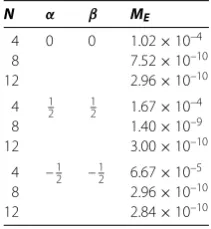
Maximum absolute errors of () subject to () and () are introduced in Table using the J-GL-C method for with various choices ofN,αandβin the interval [, ], while the absolute errors of problem () are presented in Table forα=β=,λ=λ=λ= and N= with different values of (x,t) in the interval [, ].
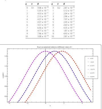
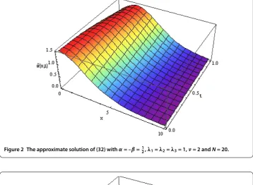
In Figure , we see that the approximate solution and the exact solution for different values oft(, . and .) of problem () are completely coinciding in the case ofα= β=,λ=λ=λ= ,ν= andN= . Moreover, the approximate solution of problem whereα= –β=,λ=λ=λ= ,ν= andN= is plotted in Figure , while the
Table 1 Maximum absolute errors withA= 0,B= 1 and various choices ofN,αandβ, for Example 1
N α β ME
4 0 0 1.02×10⁻⁴
8 7.52×10⁻¹⁰
12 2.96×10⁻¹⁰
4 12 12 1.67×10⁻⁴
8 1.40×10⁻⁹
12 3.00×10⁻¹⁰
4 –12 –12 6.67×10⁻⁵
8 2.96×10⁻¹⁰
Table 2 Absolute errors withA= 0,B= 10,α=β=12,N= 24 and various choices ofx,t, for Example 1
x t E
0 0.1 3.08×10⁻¹⁰ 1 5.33×10⁻¹¹ 2 4.53×10⁻¹¹ 3 2.13×10⁻¹¹ 4 4.37×10⁻¹¹ 5 4.37×10⁻¹¹ 6 3.57×10⁻¹¹ 7 6.56×10⁻¹¹ 8 4.77×10⁻¹¹ 9 7.96×10⁻¹¹ 10 3.08×10⁻¹⁰
x t E
0 0.2 2.87×10⁻¹⁰ 1 5.12×10⁻¹¹ 2 2.04×10⁻¹¹ 3 2.96×10⁻¹¹ 4 7.97×10⁻¹² 5 2.45×10⁻¹¹ 6 2.63×10⁻¹¹ 7 4.35×10⁻¹¹ 8 1.87×10⁻¹¹ 9 4.43×10⁻¹¹ 10 2.87×10⁻¹⁰
Figure 1 The approximate and exact solutions for different values oft(0, 0.5 and 0.9) of problem (32) withα=β=1
2,λ1=λ2=λ3= 1,ν= 2 andN= 24.
absolute error of () withα=β= –,λ=λ=λ= ,ν= andN= is displayed in Figure . This assertion that the obtained numerical results are very accurate and compare favorably with the exact solution.
Example Consider the Phi-four equation
utt=uxx+u–u, (x,t)∈D×[,T], ()
subject to initial-boundary conditions
u(A,t) =tanh
( –ν)(A–νt)
,
u(B,t) =tanh
( –ν)(B–νt)
,
Figure 2 The approximate solution of (32) withα= –β=1
2,λ1=λ2=λ3= 1,ν= 2 andN= 20.
Figure 3 The absolute error of (32) withα=β= –12,λ1=λ2=λ3= 1,ν= 2 andN= 4.
u(x, ) =tanh
( –ν)(x)
, x∈D, ()
ut(x, ) =tanh
( –ν)(x)
, x∈D. ()
The exact solution of this equation is
u(x,t) =tanh
( –ν)(x–νt)
Table 3 Maximum absolute errors withA= 0,B= 1 and various choices ofN,αandβ, for Example 2
N α β ME
4 0 0 7.38×10⁻⁴
8 1.26×10⁻⁷
12 7.20×10⁻¹²
4 12 12 11.55×10⁻⁴
8 2.49×10⁻⁷
12 1.82×10⁻¹¹
4 –12 –12 4.61×10⁻⁴
8 4.39×10⁻⁸
12 3.17×10⁻¹²
Table 4 Absolute errors withA= 0,B= 1, –α=β=12,N= 12 and various choices ofx,tfor Example 2
x t E
0 0.1 1.97×10⁻⁹ 0.1 6.05×10⁻¹¹ 0.2 6.21×10⁻¹⁰ 0.3 5.64×10⁻¹⁰ 0.4 1.04×10⁻⁹ 0.5 8.99×10⁻¹⁰ 0.6 1.31×10⁻⁹ 0.7 1.18×10⁻⁹ 0.8 1.42×10⁻⁹ 0.9 7.16×10⁻¹⁰ 1 7.89×10⁻¹¹
x t E
0 0.2 1.12×10⁻¹⁰ 1 1.49×10⁻¹⁰ 0.2 6.11×10⁻¹⁰ 0.3 6.01×10⁻¹⁰ 0.4 8.29×10⁻¹⁰ 0.5 1.08×10⁻⁹ 0.6 1.03×10⁻⁹ 0.7 1.33×10⁻⁹ 0.8 7.60×10⁻¹⁰ 0.9 2.35×10⁻¹⁰ 1 4.47×10⁻¹²
Figure 4 The approximate and exact solutions fort= 0.5 of problem (37) withα=β= –1 2,ν= 0.01
Figure 5 The approximate solution of problem (37) withα=β= –1
2,ν= 0.01 andN= 16.
Figure 6 The absolute error between the exact and approximate solutions of problem (37) where
α=β= 0,ν= 0.01 andN= 12.
Table lists the maximum absolute errors of () subject to () and (), using the J-GL-C method for with various choices ofN,αandβ. Moreover, in Table , we introduce absolute errors using the J-GL-C method for the special value –α =β = (Chebyshev polynomials of the third kind) andN= .
Table 5 Maximum absolute errors withA= 0,B= 1, and various choices ofN,αandβ, for Example 3
N α β ME
4 0 0 6.59×10⁻⁴
8 2.20×10⁻⁷
12 1.36×10⁻⁸
4 12 12 8.66×10⁻⁴
8 4.35×10⁻⁷
12 1.36×10⁻⁸
4 –12 –12 4.40×10⁻⁴
8 7.74×10⁻⁸
12 7.56×10⁻⁹
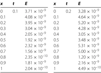
Table 6 Absolute errors withA= 0,B= 1,α=β= –12,N= 12 and various choices ofx,tfor Example 3
x t E
0 0.1 3.71×10⁻⁹ 0.1 4.08×10⁻⁹ 0.2 3.95×10⁻⁹ 0.3 3.04×10⁻⁹ 0.4 2.05×10⁻⁹ 0.5 1.92×10⁻⁹ 0.6 2.32×10⁻⁹ 0.7 1.56×10⁻⁹ 0.8 2.35×10⁻¹⁰ 0.9 1.81×10⁻⁹ 1 2.04×10⁻¹⁰
x t E
0 0.2 3.28×10⁻⁹ 0.1 4.64×10⁻⁹ 0.2 5.20×10⁻⁹ 0.3 4.28×10⁻⁹ 0.4 3.05×10⁻⁹ 0.5 3.48×10⁻⁹ 0.6 5.31×10⁻⁹ 0.7 5.00×10⁻⁹ 0.8 1.20×10⁻⁹ 0.9 2.16×10⁻⁹ 1 4.49×10⁻¹⁰
approximate solutions of problem () withα=β= (Legendre polynomials),ν= . andN= is plotted in Figure .
Example Consider the nonlinear time-dependent one-dimensional Phi-four equation in the form
utt=uxx+u–u, (x,t)∈D×[,T], ()
subject to the initial-boundary values
u(A,t) = –tanh
(A–νt)
,
u(B,t) = –tanh
(B–νt)
,
()
u(x, ) = –tanh
(x)
, x∈D,
ut(x, ) = ν –tanh
(x)
–
tanh
(x)
sech
(x)
, x∈D.
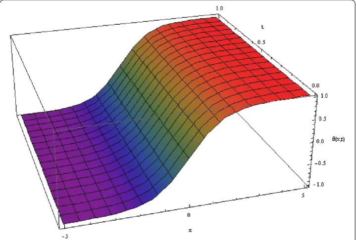
Figure 7 The approximate solution and the exact solution fort= 0.5 of problem (42) where
α=β= –12,ν= 0.01 andN= 16.
The exact solution using generalized tanh method is
u(x,t) = –tanh
(x–νt)
. ()
Maximum absolute errors of () subject to () and () are introduced in Table using the J-GL-C method for with various choices ofN,αandβ, while the absolute errors are presented in Table forα=β=(Chebyshev polynomials of the second kind) andN= at different values of (x,t).
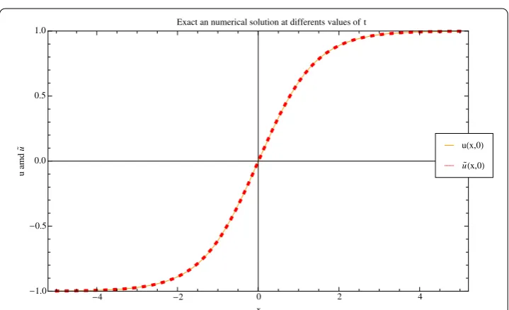
In Figure , we see that the approximate solutions and the exact solutions for three values oft(t= , ., .) of problem () are completely coincide for all values ofxin the interval x∈[–, ]. The approximate solution is plotted in Figure with values of parameters listed in its caption, and the absolute error using J-GL-C method is displayed in Figure . From the presented results, it can be concluded that the numerical solutions are in excellent agreement with the exact solutions.
5 Conclusions
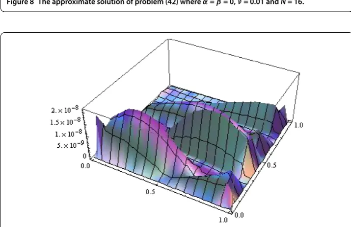
Figure 8 The approximate solution of problem (42) whereα=β= 0,ν= 0.01 andN= 16.
Figure 9 The absolute error between the exact and approximate solutions of problem (42) where
α=β=12,ν= 0.01 andN= 12.
Competing interests
The authors declare that they have no competing interests.
Authors’ contributions
The authors have equal contributions to each part of this paper. All the authors read and approved the final manuscript.
Author details
1Department of Mathematics, Faculty of Science, King Abdulaziz University, Jeddah, 21589, Saudi Arabia.2Department of Mathematics, Faculty of Science, Beni-Suef University, Beni-Suef, Egypt.3Department of Mathematics, Faculty of Science, Umm Al-Qura University, Makkah, Saudi Arabia.
Acknowledgements
This study was supported by the Deanship of Scientific Research of King Abdulaziz University. The authors would like to thank the reviewers for their constructive comments and suggestions to improve the quality of the article.
References
1. Canuto, C, Hussaini, MY, Quarteroni, A, Zang, TA: Spectral Methods: Fundamentals in Single Domains. Springer, New York (2006)
2. Doha, EH, Bhrawy, AH: An efficient direct solver for multidimensional elliptic robin boundary value problems using a Legendre spectral-Galerkin method. Comput. Math. Appl.64, 558-571 (2012)
3. Kamrani, M, Hosseini, SM: Spectral collocation method for stochastic Burgers equation driven by additive noise. Math. Comput. Simul.82, 1630-1644 (2012)
4. Saadatmandi, A, Dehghan, M: A tau approach for solution of the space fractional diffusion equation. Comput. Math. Appl.62, 1135-1142 (2011)
5. Bhrawy, AH, Alshomrani, M: A shifted Legendre spectral method for fractional-order multi-point boundary value problems. Adv. Differ. Equ.2012, Article ID 8 (2012)
6. Bhrawy, AH, Alofi, AS: The operational matrix of fractional integration for shifted Chebyshev polynomials. Appl. Math. Lett.26, 25-31 (2013)
7. Guo, BY, Yan, JP: Legendre-Gauss collocation method for initial value problems of second order ordinary differential equations. Appl. Numer. Math.59, 1386-1408 (2009)
8. Doha, EH, Bhrawy, AH, Ezz-Eldien, SS: A new Jacobi operational matrix: an application for solving fractional differential equation. Appl. Math. Model.36, 4931-4943 (2012)
9. Saadatmandi, A, Dehghan, M: The use of Sinc-collocation method for solving multi-point boundary value problems. Commun. Nonlinear Sci. Numer. Simul.17, 593-601 (2012)
10. Bhrawy, AH, Alofi, AS: A Jacobi-Gauss collocation method for solving nonlinear Lane-Emden type equations. Commun. Nonlinear Sci. Numer. Simul.17, 62-70 (2012)
11. Doha, EH, Bhrawy, AH, Hafez, RM: On shifted Jacobi spectral method for high-order multi-point boundary value problems. Commun. Nonlinear Sci. Numer. Simul.17, 3802-3810 (2012)
12. Wang, ML, Zhou, YB: The periodic wave solutions for the Klein-Gordon-Schrodinger equations. Phys. Lett. A318, 84-92 (2003)
13. Yomba, E: On exact solutions of the coupled Klein-Gordon-Schrodinger and the complex coupled KdV equations using mapping method. Chaos Solitons Fractals21, 209 (2004)
14. Li, XY, Yang, S, Wang, ML: The periodic wave solutions for the (3 + 1)-dimensional Klein-Gordon-Schrodinger equations. Chaos Solitons Fractals25, 629-636 (2005)
15. Arafa, AAM, Rida, SZ: Numerical solutions for some generalized coupled nonlinear evolution equations. Math. Comput. Model.56, 268-277 (2012)
16. Jiwari, R, Mittal, RC, Sharma, KK: A numerical scheme based on weighted average differential quadrature method for the numerical solution of Burgers’ equation. Appl. Math. Comput.219, 6680-6691 (2013)
17. Bhrawy, AH, Al-shomrani, M: A Jacobi Dual-Petrov Galerkin-Jacobi Collocation Method for Solving Korteweg-de Vries equations. Abstr. Appl. Anal.2012, Article ID 16 (2012)
18. Khan, Y: A method for solving nonlinear time-dependent drainage model. Neural Comput. Appl. (2013). doi:10.1007/s00521-012-0933-2
19. Khan, Y, Diblik, J, Faraz, N, Smarda, Z: An efficient new perturbative Laplace method for space-time fractional telegraph equations. Adv. Differ. Equ.2012, Article ID 204 (2012)
20. El-Kady, M, El-Sayed, SM, Fathy, HE: Development of Galerkin method for solving the generalized Burger’s-Huxley equation. Math. Probl. Eng.2013, Article ID 9 (2013)
21. Van Gorder, RA, Vajravelu, K: Analytical and numerical solutions of the density dependent Nagumo telegraph equation. Nonlinear Anal., Real World Appl.11, 3923-3929 (2010)
22. Dehghan, M, Mohebbi, A, Asgari, Z: Fourth-order compact solution of the nonlinear Klein-Gordon equation. Numer. Algorithms52, 523-540 (2009)
23. Chowdhury, A, Biswas, A: Singular solitons and numerical analysis of phi-four equation. Math. Sci.6, Article ID 42 (2012)
24. Sassaman, R, Biswas, A: Soliton perturbation theory for Phi-four model and nonlinear Klein-Gordon equations. Commun. Nonlinear Sci. Numer. Simul.14, 3239-3249 (2009)
25. Khater, AH, Callebaut, DK, Bhrawy, AH, Abdelkawy, MA: Nonlinear periodic solutions for isothermal magnetostatic atmospheres. J. Comput. Appl. Math.242, 28-40 (2013)
26. Soliman, AA: Exact traveling wave solution of nonlinear variants of the RLW and the PHI-four equations. Phys. Lett. A
368, 383-390 (2007)
27. Triki, H, Wazwaz, A: Envelope solitons for generalized forms of the phi-four equation. Journal of King Saud University. Science (2012). doi:10.1016/j.jksus.2012.08.001
28. Zhou, H, Shen, J: Bifurcations of travelling wave solutions for modified nonlinear dispersive phi-four equation. Appl. Math. Comput.217, 1584-1597 (2010)
29. Deng, X, Zhao, M, Li, X: Travelling wave solutions for a nonlinear variant of the Phi-four equation. Math. Comput. Model.49, 617-622 (2009)
30. Russo, M, Van Gorder, RA, Choudhury, SR: Painleve property and exact solutions for a nonlinear wave equation with generalized power-law nonlinearities. Commun. Nonlinear Sci. Numer. Simul.18, 1623-1634 (2013)
31. Van Gorder, RA, Sweet, E, Vajravelu, K: Analytical solutions of a coupled nonlinear system arising in a flow between stretching disks. Appl. Math. Comput.216, 1513-1523 (2010)
32. Doha, EH, Bhrawy, AH: A Jacobi spectral Galerkin method for the integrated forms of fourth-order elliptic differential equations. Numer. Methods Partial Differ. Equ.25, 712-739 (2009)
33. Bhrawy, AH, Alghamdi, MA: A shifted Jacobi-Gauss-Lobatto collocation method for solving nonlinear factional Langevin equation involving two fractional orders in different intervals. Bound. Value Probl.2012, Article ID 62 (2012) 34. Fan, E, Hon, YC: Generalized tanh method extended to special types of nonlinear equations. Z. Naturforsch.57a,
692-700 (2002)
doi:10.1186/1687-2770-2013-87