International Doctorate School in
Information and Communication Technologies
Department of Information Engineering and Computer Science
University of Trento
D
EEPN
EURALN
ETWORKM
ODELSFOR
I
MAGEC
LASSIFICATION ANDR
EGRESSIONSalim MALEK
THANKS
All my gratitude and thanks to God, who guided me to this way of science, and gave me the courage and the will to get to this level.
I would like to express my gratitude to my supervisor Dr. Farid Melgani for his academic and moral supports, and his valuable advices.
I thank also Dr. Yakoub Bazi and Dr. Mohamed Lamine Mekhalfi for their encouragement and support.
Abstract
Deep learning, a branch of machine learning, has been gaining ground in many research fields as well as practical applications. Such ongoing boom can be traced back mainly to the availability and the affordability of potential processing facilities, which were not widely accessible than just a decade ago for instance. Although it has demonstrated cutting-edge performance widely in computer vision, and particularly in object recognition and detection, deep learning is yet to find its way into other research areas. Furthermore, the performance of deep learning models has a strong dependency on the way in which these latter are designed/tailored to the problem at hand. This, thereby, raises not only precision concerns but also processing overheads. The success and applicability of a deep learning system relies jointly on both components. In this dissertation, we present innovative deep learning schemes, with application to interesting though less-addressed topics.
In this respect, the first covered topic is rough scene description for visually impaired individuals, whose idea is to list the objects that likely exist in an image that is grabbed by a visually impaired person, To this end, we proceed by extracting several features from the respective query image in order to capture the textural as well as the chromatic cues therein. Further, in order to improve the representativeness of the extracted features, we reinforce them with a feature learning stage by means of an autoencoder model. This latter is topped with a logistic regression layer in order to detect the presence of objects if any.
In a second topic, we suggest to exploit the same model, i.e., autoencoder in the context of cloud removal in remote sensing images. Briefly, the model is learned on a cloud-free image pertaining to a certain geographical area, and applied afterwards on another cloud-contaminated image, acquired at a different time instant, of the same area. Two reconstruction strategies are proposed, namely pixel-based and patch-based reconstructions.
From the earlier two topics, we quantitatively demonstrate that autoencoders can play a pivotal role in terms of both (i) feature learning and (ii) reconstruction and mapping of sequential data.
Convolutional Neural Network (CNN) is arguably the most utilized model by the computer vision community, which is reasonable thanks to its remarkable performance in object and scene recognition, with respect to traditional hand-crafted features. Nevertheless, it is evident that CNN naturally is availed in its two-dimensional version. This raises questions on its applicability to unidimensional data. Thus, a third contribution of this thesis is devoted to the design of a unidimensional architecture of the CNN, which is applied to spectroscopic data. In other terms, CNN is tailored for feature extraction from one-dimensional chemometric data, whilst the extracted features are fed into advanced regression methods to estimate underlying chemical component concentrations. Experimental findings suggest that, similarly to 2D CNNs, unidimensional CNNs are also prone to impose themselves with respect to traditional methods.
Contents
Chapter 1 Introduction and Thesis Overview ...1
1.1. Deep Neural Networks ...2
1.2. Applications and Open Issues ...4
1.3. Thesis Objectives, Solutions and Organization ...5
1.4. References ...7
Chapter 2 Real-Time Indoor Scene Description for the Visually Impaired Using AutoEncoder ... 10
2.1. Introduction ... 11
2.2. Coarse Description ... 13
2.3. Tools and Concepts ... 14
2.3.1 Histogram of Oriented Gradient ... 15
2.3.2 Bag of Visual Words ... 15
2.3.3 Local Binary Pattern (LBP) ... 15
2.3.4 AutoEncoder Networks (AE) ... 16
2.4. Feature Fusion ... 17
2.5. Experimental Results ... 19
2.5.1 Description of the Wearable System ... 19
2.5.2 Dataset Description ... 19
2.5.3 Evaluation Metrics and Parameter Setting ... 20
2.5.4 Results ... 21
2.6. Conclusions ... 25
2.7. References ... 26
Chapter 3 Reconstructing Cloud-Contaminated Multispectral Images with Contextualized AutoEncoder ... 28
3.1. Introduction ... 29
3.2. Methodology ... 30
3.2.1 Pixel-based Reconstruction with AutoEncoder ... 31
3.2.2 Patch-based reconstruction strategy ... 33
3.2.3 Estimation of the size of the hidden layer ... 34
3.2.4 Multi-objective Optimization ... 36
3.3. Experimental Validation ... 37
3.3.1 Dataset description... 37
3.3.2 Results ... 39
3.4. Conclusion ... 47
3.5. References ... 48
Chapter 4 1D-Convolutional Neural Networks for Spectroscopic Signal Regression ... 50
4.1. Introduction ... 51
4.2. 1D-CNNs... 52
4.2.1 Forward propagation ... 53
4.2.2 Back propagation ... 54
4.2.3 Subsampling layers ... 55
4.3. PSO-1DCNN ... 55
4.4. Prediction ... 57
4.4.1 GPR ... 57
4.4.2 SVR ... 59
4.5. Experimental results ... 60
4.5.1 Dataset description and performance evaluation ... 60
4.5.2 Parameter setting ... 63
4.5.3 Results ... 64
4.6. Conclusion ... 68
4.7. Appendix: List of Mathematical Symbols ... 69
4.8. References ... 70
Chapter 5 Convolutional SVM ... 73
5.1. Introduction ... 74
5.2. Proposed Methodology ... 75
5.2.1 Monolabel classification ... 76
5.2.2 Multilabel classification ... 77
5.3. Experimental results ... 78
5.3.1 Dataset description and performance evaluation ... 78
5.3.2 Parameter setting ... 80
5.3.3 Results ... 81
5.4. Conclusion ... 84
5.5. References ... 84
List of Figures
Figure 1-1: Example of a Restricted Boltzman Machine network ...3
Figure 1-2: Example of an AutoEncoder network ...3
Figure 1-3:Example of a simple CNN architecture ...3
Figure 2-1: Binary descriptor construction for a training image. ... 14
Figure 2-2: Pipeline of the feature learning-based image multilabeling scheme. ... 15
Figure 2-3: One layer architecture of an AE. ... 17
Figure 2-4:Diagram of the first fusion strategy (Fusion 1) based on a low-level feature aggregation. ... 18
Figure 2-5:Diagram of the second fusion strategy (Fusion 2) based on a AE induced-level aggregation. ... 18
Figure 2-6:Diagram of the third fusion strategy (Fusion 3) based on a decision-level aggregation. ... 18
Figure 2-7:View of the wearable prototype with its main components. ... 19
Figure 2-8:Impact of the threshold value on the classification rates using the three feature types. Upper row for Dataset 1, bottom row for Dataset 2. ... 21
Figure 2-9:Example of results obtained by the proposed multilabeling fusion approach for both datasets. Upper row for Dataset 1, and lower one for Dataset 2. ... 22
Figure 3-1:Proposed pixel-based AutoEncoding reconstruction method. ... 32
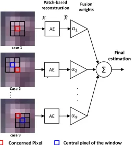
Figure 3-2:Proposed patch-based AutoEncoding reconstruction method. ... 33
Figure 3-3: Illustration of the fusion of the patch-based results related to a given pixel of interest (in black) for a 3×3 neighborhood system. In this case, 𝛼1 = 12 and all other weights 𝛼2 = ⋯ = 𝛼9 = 116. ... 34
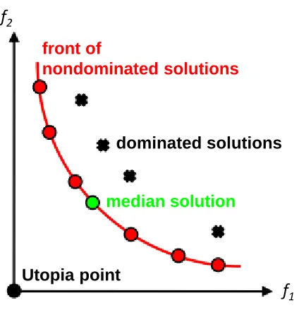
Figure 3-4: Illustration of a front of nondominated solutions. ... 37
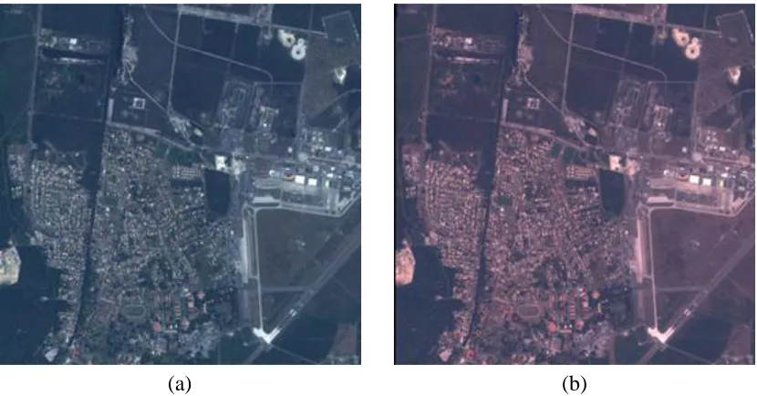
Figure 3-5: Color composite of first dataset acquired by FORMOSAT-2 over the Arcachon basin on (a) 24th June and (b) 16th June, 2009. ... 38
Figure 3-6: Color composite of second dataset acquired by SPOT-5 over the Réunion island on (a) May 2nd and (b) June 18th, 2008. ... 38
Figure 3-7: Masks adopted to simulate the different ground cover contaminations... 39
Figure 3-8: Pareto fronts obtained at convergence for the first dataset and mask A simulation by (a) pixel-based autoencoding reconstruction, and (b) patch-based autoencoding reconstruction. ... 40
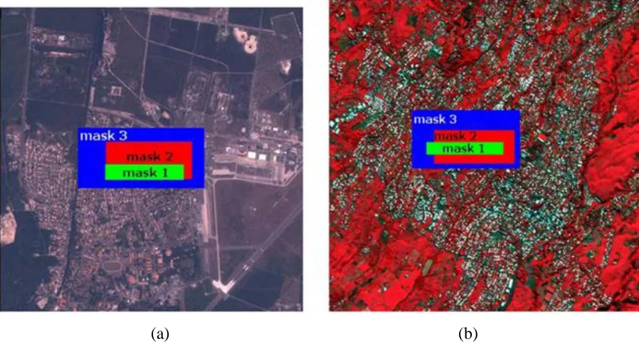
Figure 3-9: Masks adopted to simulate the different sizes of contamination. ... 42
Figure 3-10: Examples of qualitative results for Dataset 1. (a) Original image. Image reconstructed (after contamination with mask C) by the (b) OMP and (c) patch-based reconstruction methods. ... 44
Figure 3-11: Examples of qualitative results for Dataset 2. (a) Original image. Image reconstructed (after contamination with mask 2) by the (b) OMP and (c) patch-based reconstruction methods. ... 44
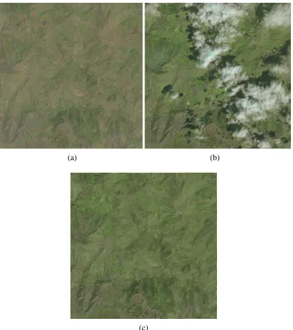
Figure 3-12: Color composite of the third dataset acquired by Sentinel-2 over Washington on (a) September 14th, 2015 (source image); (b) August 5th, 2015 (target image 1); and (c) July 20th, 2016 (target image 2). ... 45
Figure 3-13: Masked clouds and shadows of the third dataset. ... 45
Figure 3-14: Reconstructed images obtained for dataset 3. (a) second image (August 5th, 2015), (b) third image (July 20th, 2016). ... 46
Figure 3-15: Zooms of reconstruction results obtained for third image (July 20th, 2016) from source image (September 14th, 2015) of dataset 3, over (a)-(b) urban and (d)-(e) green areas. For comparison, results generated by the OMP method are provided in (c) and (f). ... 46
Figure 3-16: Results achieved for dataset 4. (a) first image (July 31st, 2016), (b) second image (March 28th, 2016), (c) reconstruction of second image. ... 47
... 53
Figure 4-3:Architecture of the PSO-1DCNN. ... 56
Figure 4-4: Near-infrared spectra of orange juice training samples. ... 61
Figure 4-5: Mid-infrared spectra of wine training samples. ... 61
Figure 4-6: Near-infrared spectra of Tecator training samples. ... 62
Figure 4-7: Effect of number of layers on estimation error. ... 64
Figure 4-8: Effect of number of feature signals on estimation error. ... 64
Figure 4-9: Sample-by-sample comparison between estimated and real output values for the test set of the Orange Juice dataset. ... 67
Figure 4-10: Sample-by-sample comparison between estimated and real output values for the test set of the Wine dataset. ... 67
Figure 4-11: Sample-by-sample comparison between estimated and real output values for the test set of the Tecator dataset ... 68
Figure 5-1: Estimating the weights of the convolution layer with SVM for detecting the presence of two objects in a given input image. ... 75
Figure 5-2: Training set generation for the first convolution layer. ... 76
Figure 5-3: Supervised feature map generation. ... 77
Figure 5-4: Example of fusion of output maps of two CNNs ... 78
Figure 5-6: Example of images of the first dataset ... 79
Figure 5-7: Example of images of the second dataset ... 79
Figure 5-8: Example of images of the third dataset ... 79
Figure 5-9: Example of classification results with CSVM and GoogLeNet on Dataset1. In red are highlighted false positives. ... 82
Figure 5-10: Example of classification results with CSVM and ResNet on Dataset2. In red are highlighted false positives. ... 82
List of Tables
Table 2-1: Obtained recognition results using single features. ... 21
Table 2-2: Classification outcomes of all the fusion schemes. ... 22
Table 2-3: Comparison of classification rates on Dataset 1. ... 23
Table 2-4: Comparison of classification rates on Dataset 2. ... 23
Table 2-5: Comparison of classification rates on Dataset 1 under different resolutions. ... 24
Table 2-6: Comparison of classification rates on Dataset 2 under different resolutions. ... 24
Table 2-7: Comparison of average runtime per image on Dataset 1 under different resolutions. ... 24
Table 2-8: Comparison of average runtime per image on Dataset 2 under different resolutions. ... 25
Table 3.1: Best size of hidden layer found for the different cases... 40
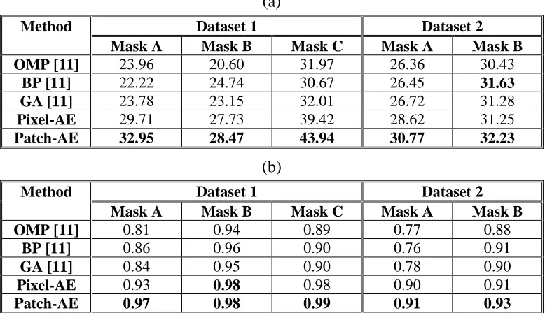
Table 3.2: (a) PSNR values and (b) correlation coefficients obtained by the different methods in the first simulation experiments. ... 41
Table 3.3: Analysis of the sensitivity to the patch size in terms of PSNR for the first simulation experiments. 1×1 size refers to the pixel-based strategy. ... 41
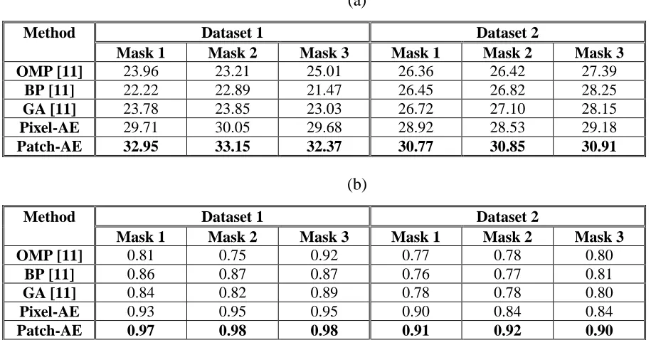
Table 3.4: (a) PSNR values and (b) correlation coefficients obtained by the different methods in the second simulation experiments. ... 43
Table 3.5: Analysis of the sensitivity to the patch size in terms of PSNR for the second simulation experiments. 1×1 size refers to the pixel-based strategy. ... 44
Table 4.1: Best parameter values of the 1D-CNN for each dataset. ... 63
Table 4.2:Best parameter values of the PSO-1DCNN for each dataset... 63
Table 4.3:Results for the Orange Juice dataset. ... 65
Table 4.4:Results for the Wine dataset. ... 65
Table 4.5:Results for the Tecator dataset. ... 65
Table 4.6:Gain in accuracy for the 3 datasets. ... 65
Table 5.1:Best parameter values of the CSVM for each dataset. ... 80
Table 5.2:Comparison of classification rates on Dataset 1. ... 81
Table 5.3:Comparison of classification rates on Dataset 2. ... 81
Table 5.4:Comparison of classification rates on Dataset 3. ... 81
Table 5.5:Training time of the proposed CSVM. ... 83
Table 5.6:Comparison of average runtime per image on Dataset 1... 83
Table 5.7:Comparison of average runtime per image on Dataset 2... 83
1
Chapter 1
2 1.1. Deep Neural Networks
Machine learning is a study field of artificial intelligence (AI) that enables systems to automatically learn and improve from experience without or with little explicit human interference. It focuses on the development of computer programs that can acquire data and build models in order to make better decisions according to prior observations or data records.
According to the adopted learning way, machine learning methods are usually categorized as being either supervised or unsupervised. In supervised learning, a model at hand is learned on a certain data along with its respective labels. Thus, once a model is learned on known data, it can be further fed with another set of data whose labels are unknown. In unsupervised learning, however, prior labels are inaccessible or accessible but unimportant for the application being addressed. This latter, thus, consists in studying how systems can infer functions to define hidden structures from unlabeled data. Semi-supervised learning is another direction whose aim is to exploit a small-sized label data and a large-sized unlabeled data.
A close look at the recent literature would tell that a big focus is being oriented towards deep learning. By contrast to traditional Neural Networks, various layers of neurons in deep learning perform a hierarchical learning of the data representation via non-linear transformations. In other words, the data is passed cumulatively across a long chain of layers (thus, the description deep), where each layer can be fully or partially connected to the preceding one.
Although deep architectures have long existed, the term “deep learning” was first introduced in
2006 by Hinton et al. [1], where they showed that a multilayer feedforward neural network can be more
efficient by applying pretraining of one layer at a time and considering each layer as an unsupervised Restricted Boltzmann Machine (RBM), by using supervised back propagation for finetuning. One year
later, Bengio et al. [2] developed the Stacked AutoEncoder (SAE), which is a deep architecture based on
the concatenation of many AutoEncoders (AEs). Each AE has three layers, one visible layer (input), one hidden layer and one reconstruction layer with similar size as the input. Another famous deep architecture is the Convolutional Neural Network (CNN) [3]. CNNs are generally composed of many layers, where each layer has two parts, one for convolution (filtering) and one for pooling (subsampling). The chain of convolutional/pooling layers is normally concluded by a regression layer (e.g., logistic regression) in order to discern the class label of the image/object presented as input to the network. CNNs are shaped in a 2D structure, which offers the advantage of directly processing the raw images. This can be achieved with local connections and tied weights followed by subsampling. Yet, it is evident that deep models in general, and CNNs in particular, undergo a heavy processing, which demands highly powerful computation machines.
3 Figure 1-1: Example of a Restricted Boltzman Machine network.
Figure 1-2: Example of an AutoEncoder network.
Figure 1-3:Example of a simple CNN architecture.
h1 h2 h3 h4
v1 v2 v3 v4 v5
h∈{0,1}4
v∈{0,1}5
W∈ ℝ4x5
Visible layer Hidden layer
h1
h2
h3 x1
x2
x3
x4
Hidden layer
Input layer Reconstruction layer
+1
+1
C1
Input 32x32
F1: feature map
4@28x28 F2: f. map
4@14x14 F3: f. map
8@10x10 F4: f. map 8@5x5
5x5 convolution
S1 2x2 subsampling
C2 5x5 convolution
S2 2x2 subsampling
Feature extraction
Neural Network
4 1.2. Applications and Open Issues
Deep learning techniques have been suggested to solve problems related to diverse research fields. For instance, in robotics, CNN was used in order to recognize the category and estimate the pose of garments hanging from a single point [4] and for real-time human detection with a feature-based layered pre-filter [5]. On the other hand, SAE was used for dimension reduction and combined with particle filter
for real-time humanoid robot imitation [6]. In the remote sensing field, Huang et al. [7] proposed a new
pan-sharpening method based on SAEs to address the remote sensing image fusion problem. Tang et al.
[8] propose a method for ship detection based on a Stacked Denoising Autoencoder (SDA) for hierarchical ship feature extraction in the wavelet domain and extreme learning machine (ELM) for
feature fusion and classification. Chen et al. [9] combine SAEs with principal component analysis (PCA)
to learn deep features of hyperspectral images, they propose to extract spatial dominated information for the classification and use the PCA to reduce the large input dimension. A logistic regression is used as output layer for the classification. Fang et al. [10] use CNNs for scene classification, CaffeNet [11] is used as pretrained model in the classification architecture and finetuning is applied to the pretrained model in order to tailor it to scene classification. Regarding problems of detection and recognition, deep learning was widely used to solve problems of different nature such as speech recognition [12]-[14], face recognition [15]-[18], traffic signs [19]-[21], pedestrian detection and recognition [22]-[24] and detection of various objects [25]-[28]. In the biomedical field, RBM and SAEs were used to solve problems of abnormalities detection and classification of Electrocardiogram signals (ECG) [29]-[32], Electroencephalogram signals (EEG) [33]-[35], Electrooculogram signals (EOG) [36]-[37] and Electromyogram signals (EMG) [38].
5 A second argument constituting this dissertation relates to remote sensing, where only several recent works deal with the problem of clouds based on a deep learning approach [45]-[46]. For instance, all focus on the problem of cloud detection, whilst none, to the best of our awareness, tried to solve the problem of removing clouds and reconstructing the missing area (the area obscured by clouds). Such contribution can bring benefits for many applications, especially with those which deal with multitemporal images.
Another important field of research is chemometrics analyses from spectroscopic data. Usually researchers use reference methods of regression such as partial least squares regression (PLS regression), support vector machines for regression (SVR) and Gaussian process regression (GPR) in order to estimate the concentration of chemical components of interest in a given product. By introducing deep learning, chemometrics can benefit from the advantages that deep methods can provide, especially the capacity of extracting highly discriminative features.
The last concern of this dissertation relates to the manner that deep methods, especially CNNs, estimate the parameters of the network. As a matter of fact, they are all based on the back propagation of errors, which requires big training data and numerous iterations to converge to a satisfactory solution. Such situation involves the need for sophisticated hardware and long processing time. Thus, it would be of particular interest to find another solution to train the network in order to overcome such inconvenient and even handle small training datasets.
1.3. Thesis Objectives, Solutions and Organization
As mentioned earlier, deep learning was used in many research fields and applications and brought important improvements and contributions. However, in some application issues, deep learning methods cannot necessarily be directly applied as they may need some modification and improvement to be suited to the considered problems. To this end, we propose to use deep methods to solve problems related to (i) multilabel classification for scene description for the visually impaired (VI) people, (ii) reconstructing areas obscured by clouds in multispectral images, and (iii) chemometric analysis from spectroscopic data.
6 Once generated, the new features are fed into a logistic regression layer using a multilabeling strategy as to draw the final outcomes highlighting the objects present in the image of interest.
For the problem of cloud removal and consequent reconstruction of obscured areas in multispectral images, we propose to exploit the strength of the AE networks in the reconstruction phase to restore the missing data. Suppose we have two satellite images of the same area, taken at two different times. Let the first be the cloud-free image (reference image) and the second be the cloud-contaminated image (target image), the AE learning will be slightly modified in such a way that, rather than supposing that the output layer (the reconstruction layer) is equal to the input layer, we consider here that the output is constituted of pixels from the target image, and their corresponding pixels on the reference image are used as input. In other words, we try to find the essential mapping function between the reference and the target images using the AE.
Concerning the question of chemometrics analyses from spectroscopic data, we propose to profit from the advantages of CNNs in extracting high discriminative features from images to apply them on spectroscopic data. Since the concerning data is of one-dimensional nature, the architecture of the CNN is modified and adapted to fulfill spectroscopic data requirements. In particular, filtering and pooling operations as well as equations for training are revisited. Furthermore, we propose to use the particle swarm optimization (PSO) method to train the 1D-CNN.
As per the last concern of this thesis, we propose a new method to calculate the weights of the CNN kernels. The method consists in training an SVM for each kernel in the CNN. The advantage of this new way of training is the possibility to use small training dataset while retaining a satisfactory performance of the network. Furthermore, the training is applied in one pass i.e., just one iteration, which renders it so fast compared to conventional CNNs.
The remainder of this dissertation is outlined as follows. Chapter 2 describes the multilabeling method using the AEs to describe the indoor environment for VI persons. In chapter 3, we give details about the proposed method to reconstruct a missing area covered by clouds in multispectral images using AEs. Chapter 4 details the developed 1D-CNN for chemometric data analysis. In Chapter 5, we present the developed SVM_CNN for multilabel classification. Finally, Chapter 6 concludes the thesis and gives suggestions for possible future improvements.
Finally, we would like to mention that, although deep learning constitutes a denominator of all the addressed topics in this thesis, the applications remain conceptually distinct. Thus, the following chapters were conducted independently. That is, each chapter is self-contained, which eases access to the reader and removes the need of keeping track of the chapters in a sequential order. Nevertheless, we suppose that the reader is familiar with typical concepts related to computer vision and machine learning. Otherwise, the reader is recommended to consult the references provided in each chapter.
7 1.4. References
[1] G. E. Hinton, S. Osindero and Y. W. Teh, "A Fast Learning Algorithm for Deep Belief Nets," in Neural Computation, vol. 18, no. 7, pp. 1527-1554, July 2006.
[2] Y. Bengio, P. Lamblin, D. Popovici, and H. Larochelle, “Greedy layer-wise training of deep networks,” in Proc. Neural Inf. Process. Syst., Cambridge, MA, USA, , pp. 153–160, 2007.
[3] Y. Lecun, L. Bottou, Y. Bengio and P. Haffner, "Gradient-based learning applied to document recognition," in Proceedings of the IEEE, vol. 86, no. 11, pp. 2278-2324, Nov 1998.
[4] I. Mariolis, G. Peleka, A. Kargakos and S. Malassiotis, "Pose and category recognition of highly deformable objects using deep learning," 2015 International Conference on Advanced Robotics (ICAR), Istanbul, 2015, pp. 655-662.
[5] E. Martinson and V. Yalla, "Real-time human detection for robots using CNN with a feature-based layered pre-filter," 2016 25th IEEE International Symposium on Robot and Human Interactive Communication (RO-MAN), New York, NY, 2016, pp. 1120-1125.
[6] Y. Kondo and Y. Takahashi, "Real-time whole body imitation by humanoic robot based on particle filter and dimension reduction by autoencoder," 2017 Joint 17th World Congress of International Fuzzy Systems Association and 9th International Conference on Soft Computing and Intelligent Systems (IFSA-SCIS), Otsu, 2017, pp. 1-6.
[7] W. Huang, L. Xiao, Z. Wei, H. Liu and S. Tang, "A New Pan-Sharpening Method With Deep Neural Networks," in IEEE Geoscience and Remote Sensing Letters, vol. 12, no. 5, pp. 1037-1041, May 2015.
[8] J. Tang, C. Deng, G. B. Huang and B. Zhao, "Compressed-Domain Ship Detection on Spaceborne Optical Image Using Deep Neural Network and Extreme Learning Machine," in IEEE Transactions on Geoscience and Remote Sensing, vol. 53, no. 3, pp. 1174-1185, March 2015.
[9] Y. Chen, Z. Lin, X. Zhao, G. Wang and Y. Gu, "Deep Learning-Based Classification of Hyperspectral Data," in IEEE Journal of Selected Topics in Applied Earth Observations and Remote Sensing, vol. 7, no. 6, pp. 2094-2107, June 2014.
[10] Z. Fang, W. Li, J. Zou and Q. Du, "Using CNN-based high-level features for remote sensing scene classification," 2016 IEEE International Geoscience and Remote Sensing Symposium (IGARSS), Beijing, 2016, pp. 2610-2613.
[11] Y. Jia, E. Shelhamer, J. Donahue, S. Karayev, J. Long, and R. Girshick, ''Caffe: Convolutional architecture for fast feature embedding," arXiv preprint arXiv:1408.5093,2014.
[12] M. Cai, Y. Shi and J. Liu, "Deep maxout neural networks for speech recognition," 2013 IEEE Workshop on Automatic Speech Recognition and Understanding, Olomouc, 2013, pp. 291-296.
[13] S. Kundu, G. Mantena, Y. Qian, T. Tan, M. Delcroix and K. C. Sim, "Joint acoustic factor learning for robust deep neural network based automatic speech recognition," 2016 IEEE International Conference on Acoustics, Speech and Signal Processing (ICASSP), Shanghai, 2016, pp. 5025-5029.
[14] P. Harár, R. Burget and M. K. Dutta, "Speech emotion recognition with deep learning," 2017 4th International Conference on Signal Processing and Integrated Networks (SPIN), Noida, 2017, pp. 137-140.
[15] D. Menotti et al., "Deep Representations for Iris, Face, and Fingerprint Spoofing Detection," in IEEE Transactions on Information Forensics and Security, vol. 10, no. 4, pp. 864-879, April 2015.
[16] S. Gao, Y. Zhang, K. Jia, J. Lu and Y. Zhang, "Single Sample Face Recognition via Learning Deep Supervised Autoencoders," in IEEE Transactions on Information Forensics and Security, vol. 10, no. 10, pp. 2108-2118, Oct. 2015.
8 [18] X. Peng, N. Ratha and S. Pankanti, "Learning face recognition from limited training data using deep neural networks," 2016 23rd International Conference on Pattern Recognition (ICPR), Cancun, 2016, pp. 1442-1447.
[19] C. Li and C. Yang, "The research on traffic sign recognition based on deep learning," 2016 16th International Symposium on Communications and Information Technologies (ISCIT), Qingdao, 2016, pp. 156-161.
[20] R. Q. Qian, Y. Yue, F. Coenen and B. L. Zhang, "Traffic sign recognition using visual attribute learning and convolutional neural network," 2016 International Conference on Machine Learning and Cybernetics (ICMLC), Jeju, 2016, pp. 386-391.
[21] F. Lin, Y. Lai, L. Lin and Y. Yuan, "A traffic sign recognition method based on deep visual feature," 2016 Progress in Electromagnetic Research Symposium (PIERS), Shanghai, 2016, pp. 2247-2250.
[22] B. Peralta, L. Parra and L. Caro, "Evaluation of stacked autoencoders for pedestrian detection," 2016 35th International Conference of the Chilean Computer Science Society (SCCC), Valparaiso, 2016, pp. 1-7.
[23] D. O. Pop, A. Rogozan, F. Nashashibi and A. Bensrhair, "Incremental Cross-Modality deep learning for pedestrian recognition," 2017 IEEE Intelligent Vehicles Symposium (IV), Los Angeles, CA, 2017, pp. 523-528.
[24] A. Dominguez-Sanchez, M. Cazorla and S. Orts-Escolano, "Pedestrian Movement Direction Recognition Using Convolutional Neural Networks," in IEEE Transactions on Intelligent Transportation Systems, vol. PP, no. 99, pp. 1-9, 2017.
[25] X. Wang, M. Yang, S. Zhu and Y. Lin, "Regionlets for Generic Object Detection," in IEEE Transactions on Pattern Analysis and Machine Intelligence, vol. 37, no. 10, pp. 2071-2084, Oct. 1 2015.
[26] F. Deng, X. Zhu and J. Ren, "Object detection on panoramic images based on deep learning," 2017 3rd International Conference on Control, Automation and Robotics (ICCAR), Nagoya, 2017, pp. 375-380.
[27] B. Tian, L. Li, Y. Qu and L. Yan, "Video Object Detection for Tractability with Deep Learning Method," 2017 Fifth International Conference on Advanced Cloud and Big Data (CBD), Shanghai, 2017, pp. 397-401.
[28] F. A. Chang, C. C. Tsai, C. K. Tseng and J. I. Guo, "Embedded multiple object detection based on deep learning technique for advanced driver assistance system," 2017 IEEE 60th International Midwest Symposium on Circuits and Systems (MWSCAS), Boston, MA, 2017, pp. 172-175.
[29] M. A. Rahhal, Y. Bazi, H. AlHichri, N. Alajlan, F. Melgani and R. R Yager, “Deep learning approach for
active classification of electrocardiogram signals,” Information Sciences 345, 340–354, 2016.
[30] P. R. Muduli, R. R. Gunukula and A. Mukherjee, "A deep learning approach to fetal-ECG signal reconstruction," 2016 Twenty Second National Conference on Communication (NCC), Guwahati, 2016, pp. 1-6.
[31] Z. Wu et al., "A Novel Features Learning Method for ECG Arrhythmias Using Deep Belief Networks," 2016 6th International Conference on Digital Home (ICDH), Guangzhou, 2016, pp. 192-196.
[32] Lin Zhou, Yan Yan, Xingbin Qin, Chan Yuan, Dashun Que and Lei Wang, "Deep learning-based classification of massive electrocardiography data," 2016 IEEE Advanced Information Management, Communicates, Electronic and Automation Control Conference (IMCEC), Xi'an, 2016, pp. 780-785.
[33] Z. Yin and J. Zhang, "Recognition of Cognitive Task Load levels using single channel EEG and Stacked Denoising Autoencoder," 2016 35th Chinese Control Conference (CCC), Chengdu, 2016, pp. 3907-3912.
[34] L. Fraiwan and K. Lweesy, "Neonatal sleep state identification using deep learning autoencoders," 2017 IEEE 13th International Colloquium on Signal Processing & its Applications (CSPA), Penang, Malaysia, 2017, pp. 228-231.
9 [36] L. H. Du, W. Liu, W. L. Zheng and B. L. Lu, "Detecting driving fatigue with multimodal deep learning," 2017 8th International IEEE/EMBS Conference on Neural Engineering (NER), Shanghai, 2017, pp. 74-77.
[37] Bin Xia et al., "Electrooculogram based sleep stage classification using deep belief network," 2015 International Joint Conference on Neural Networks (IJCNN), Killarney, 2015, pp. 1-5.
[38] A. Ben Said, A. Mohamed, T. Elfouly, K. Harras and Z. J. Wang, "Multimodal Deep Learning Approach for Joint EEG-EMG Data Compression and Classification," 2017 IEEE Wireless Communications and Networking Conference (WCNC), San Francisco, CA, 2017, pp. 1-6.
[39] T. Grigorios, and K. Ioannis, "Multi-label classification: an overview," International Journal of Data Warehousing & Mining. Vol. 3, no. 3, 2007, pp. 1–13.
[40] Z. Min-Ling, Z. Zhi-Hua, "A review on multi-label learning algorithms", IEEE Trans. Knowl. Data Eng., vol. 26, no. 8, pp. 1819-1837, Aug. 2014
[41] J. Read, B. Pfahringer, G. Holmes, and E. Frank, “Classifier Chains for Multi-label Classification,” Machine Learning Journal. Springer. Vol. 85, no. 3, 2011.
[42] W. W. Cheng, E. Hullermeier, "Combining instance-based learning and logistic regression for multilabel classification", Mach. Learn., vol. 76, no. 2/3, pp. 211-225, Sep. 2009.
[43] R. E. Schapire, Y. Singer, "Improved boosting algorithms using confidence-rated predictions", Mach. Learn., vol. 37, no. 3, pp. 297-336, Dec. 1999.
[44] A. Elisseeff, J. Weston, "A kernel method for multi-labelled classification", Adv. Neural Inf. Process. Syst. 14, vol. 14, pp. 681-687, 2002.
[45] F. Xie, M. Shi, Z. Shi, J. Yin and D. Zhao, "Multilevel Cloud Detection in Remote Sensing Images Based on Deep Learning," IEEE Journal of Selected Topics in Applied Earth Observations and Remote Sensing, vol. 10, no. 8, pp. 3631-3640, Aug. 2017.
10
Chapter 2
11 2.1. Introduction
Strolling around, adjusting the walking pace and bodily balance, perceiving nearby or remote objects and estimating their depth, are all effortless acts for a well-sighted person. That is, however, hardly doable for other portions in society, such as individuals with certain cases of handicap, or visual impairment, which may require different forms of substantial training, and in many situations external physical and/or verbal intervention as to ease their mobility. In dealing with that, numerous attempts at different governmental, institutional, as well as societal spheres have been taking place.
One assistive line, ought to be undertaken by various research institutions, is the providence of either technological designs or end-user products that can help bridging the gap between the conditions being experienced by such disabled people and their expectations. As per the physically handicapped category, a well-established amount of rehabilitation (particularly robotic-based) layouts has been developed so far. However, when it comes to blindness rehabilitation technologies, relatively fewer attentions have been drawn in the relevant literature. As a side note, depending upon the severity of sight loss, vision disability is an umbrella term that encompasses a wide range of progressively inclusive cases, since it could be diagnosed as a: (i) mild impairment, (ii) middle-range impairment, (iii) severe impairment, and ends up to the unfortunate (iv) full blindness. Full sight loss is therefore a serious disability that entails far-reaching ramifications, as it blocks in many cases, the affected individual from conducting his/her daily routines smoothly.
In order to enable the visually disabled persons to move around more easily, several contributions have been proposed in the literature, which are commonly referred to as Electronic Travel Aids (ETAs). By and large, the current ETA methodologies can be identified according to two distinct but complementary aspects, namely: (i) mobility and navigation assistance, that undertakes as a goal assisting visually disabled people to autonomously walk around with the possibility to sense nearby obstacles, and avoid potential collisions thereby, and (ii) object recognition, whose underlying motive is to aid them recognize objects.
12 is present along the walking path. The concept of the ultrasonic sensors is that they simultaneously emit beams of signals, which in case of obstacles if any, are reflected back. The distance to the obstacles is then deduced based on the time lapse between emission and reflection (commonly termed as time of flight − TOF). The same concept was adopted in [4], where the sensors are placed on a wearable belt instead. Another similar work was put forth in [5]. In this work, the sensors were placed on the shoulders of the user as well as on a guide cane. Another unique contribution proposes exploiting electromagnetic signals instead of ultrasonic ones by using a widespread antenna [6]. However, the capacity of the proposed prototype is limited to 3 m ahead of the user. Having a close look at the literature, it emerges clearly that TOF-based concepts have often been employed and exhibited promising outcomes. The apparent downsides of such methodologies, however, are mainly confined to the dimensions as well as weight of the developed prototypes on the one hand, which may compromise the user’s convenience, and the demanding power consumption (i.e., constant emission/reception of ultrasonic signals) on the other hand.
Regarding the object recognition aspect, introspectively far less contributions can be observed. This might be traced back to the reason that object recognition for the blind might be a harder task to fulfil as compared to navigation and object avoidance. In other words, mobility and object avoidance does not pay attention to the kind of potential objects but to their presence instead, whilst object recognition emphasises on the nature of the nearby objects (i.e., not only their existence). Furthermore, recognizing objects, in camera-shot images, might come at the cost of several challenges such as rotation, scale, and illumination variations, notwithstanding the necessity to carry out such task in a brief time lapse. Nevertheless, different computer-vision techniques have been tailored to tackle this issue. In [7], for instance, a food product recognition system in shopping spaces was proposed. It relies on detecting and recognizing the QR codes of food items by means of a portable camera. Another work considers detecting and recognizing bus line numbers for the VI [8]. Banknote recognition has also been addressed in [9]. Staircases, doors, and indoor signage detection/ recognition have been considered in [10–12]. In [13], the authors developed a prototype composed of ultrasonic sensors and a video camera, which is embedded in a smartphone for a real-time obstacle detection and classification. They first extract FAST feature points from the image and track them with a multiscale Lucas-Kanade algorithm. Then, in the classification phase, a Support Vector Machine was used to detect one of the four objects defined a priori. Consequently, it can be observed that the scarce amount of works that have been devoted to assisted object recognition for the VI so far, emphasize on detecting/recognizing single classes of objects. On this point, it is believed that extending the process into a multiobject recognition is prone to provide a richer description for the VI people.
13 limitation, Mekhalfi et al. [14] introduced a novel approach called coarse description, which operates on portable camera-grabbed images by listing the objects existing in a given nearby indoor spot, irrespective of their location in the indoor space. Precisely, they proposed Scale Invariant Feature Transform (SIFT), Bag of Words (BOW), and Principal Component Analysis (PCA) strategies as a means of image representation. For the sake of furthering the performance of their coarse image description, they suggested another scheme, which exploits Compressive Sensing (CS) theory for image representation and a semantic similarity metric for image likelihood estimation through a bunch of learned Gaussian Process Regression (GPR) models, and concluded that a trade-off between reasonable recognition rates and low processing times can be maintained [15].
In this Chapter, we propose a new method to describe the surrounding environment for a VI person in real-time. We use Local Binary Pattern (LBP) technique, Histogram of Oriented Gradient (HOG) and BOW to describe coarsely the content of the image acquired via an optical camera. In order to improve the state of the art results and deal properly with runtime, we propose to use a deep learning approach, in particular an Auto Encoder Neural Network (AE), to create a new high-level feature representation from the previous low-level features (HOG, BoW and LBP). Once generated, the new feature vectors are fed into a logistic regression layer using a multilabeling strategy as to draw the objects present in the image of concern. This work is a part of a project to guide a VI person in an indoor environment. As validated by the experimental setup, tangible recognition gains and significant speedups have been scored with respect to recent works.
In what follows, Section 2.2 recalls the coarse scene description in brief. Section 2.3 provides short but self-contained conceptual backgrounds of the different methodologies employed for image representation. Section 2.4 outlines the image multilabeling pipeline, which is meant for coarse description. In Section 2.5, we quantify the recognition rates and the processing time and discuss the different pros and cons of the proposed method in the context of indoor scene description. Finally, conclusions are given in Section 2.6.
2.2. Coarse Description
14 Figure 2-1: Binary descriptor construction for a training image.
2.3. Tools and Concepts
Let us consider a colour image X acquired by a portable digital camera in an indoor environment. Due to several inherent properties of the images, such as illumination, rotation and scale changes, the images cannot be used in their raw form but need to be transformed into an adequate feature space that is able to capture the spatial as well as the spectral variations. Such objective can normally be addressed from three perspectives, namely: (i) shape information, (ii) colour information, and (iii) textural changes. On this point, adopting one feature modality while omitting the others may drop the robustness of the classification algorithm being developed. We therefore resort to a more efficient representation, by making use of all three feature modalities. Precisely, we opt for reputed feature extractors. The first one is the HOG [16] to feature the different shapes distributed over the images. The second one is the BOW [17] based on colour information of the different chromatic channels (BOW_RGB). Finally, the LBP technique in order to express the textural behaviour of the images. As a matter of fact, all the mentioned features can yield interesting results, and this has been documented by previous works, mainly related to object, texture recognition, biometrics as well as remote sensing. In order to further boost their representativeness, we also put forth a feature learning scheme that maps the original feature vectors (derived by means of either feature type mentioned above) onto another lower/higher feature space that offers a better feature representation capability. A well-established feature learning model is the Stacked AutoEncoder (SAE) neural network, or simply AutoEncoder (AE), which constructs a model learned on features pertaining to training images, and then applies it on a given image in order to produce a final image representation.
15 Figure 2-2: Pipeline of the feature learning-based image multilabeling scheme.
2.3.1 Histogram of Oriented Gradient
The HOG was initially aimed at pedestrian detection [16]. Soon later, it was utilized in other applications ranging from object recognition and tracking to remote sensing [18,19]. The basic idea of the HOG is to gather the gradient variations across a given image. Basically, this can be done by dividing the image into adjacent small-sized areas, called cells, and calculating the histograms of the magnitudes/directions of the gradient for the pixels within the cell. Each pixel of the cell is then assigned to one of the bins of the histogram, according to the orientation of the gradient at this point. This assignment is weighted by the gradient of the intensity at that point. Histograms are uniform from either 0 to 180° (unsigned case) or from 0 to 360° (signed case). Dalal and Triggs [16] point out that a fine quantization of the histogram is needed, and they get their best results with a 9-bin histogram. The combination of the computed histograms then forms the final HOG descriptor.
2.3.2 Bag of Visual Words
The BOW is a very popular model in the general computer vision literature. It is usually adopted for its notable property of promoting a concise but rich representation of a generic image. BOW signatures are generally reproduced from a certain feature space of the images, it can be the spectral intensities or alternatively keypoint-based descriptors derived from the images. The BOW is opted for in our work in order to produce a compact representation of the colour attributes of an image. We therefore depart from the chromatic (Red, Green, and Blue channels) values of the images. At first, a basis commonly referred to as codebook is established by gathering all the spectral features of the training images into a matrix. Afterwards, we apply a clustering technique i.e., the K-means clustering, on the built matrix to narrow down its size, which points out a small-sized basis (codebook). Next, the occurrences of the elements (words) of the codebook are observed in the chromatic space of a given image, which turns out to generate a compact histogram whose length equals to the number of the codebook’s words. For a more detailed explanation, the reader is referred to [14,17].
2.3.3 Local Binary Pattern (LBP)
Texture is a very important information that can play a key-role in characterizing images and their objects. One of the most popular techniques in this regard is the Local Binary Pattern (LBP) which is a multiresolution, gray-scale, and rotation invariant texture representation. It was first proposed by Ojala et al. [20] and then improved by Guo et al. [21] who introduced a variant called Completed Local Binary Pattern (CLBP), followed by many other variants. The following part gives a brief review about the basic
16
LBP operator. Given a pixel in the image z(u, v) its LBP code is computed by comparing its intensity
value to the values of its local neighbours:
𝐿𝐵𝑃𝑃,𝑅(𝑢, 𝑣) = ∑𝑃−1𝑝=0𝐻(z(𝑢, 𝑣) − z(𝑢𝑝, 𝑣𝑝))2𝑝 (2.1)
where z(𝑢𝑝, 𝑣𝑝) is the grey value of its pth neighbouring pixel, P is the total number of neighbours, R is the radius of the neighbourhood and H(∙) is the Heaviside step function.
The coordinates of the neighbour z(𝑢𝑝, 𝑣𝑝) are: 𝑢𝑝 = 𝑢 + 𝑅cos (2π𝑝
𝑃 ) and 𝑣𝑝 = 𝑣 − 𝑅sin (
2π𝑝 𝑃 ). If the neighbors do not fall at integer coordinates, the pixel value is estimated by interpolation. Once the LBP label is constructed for every pixel z(𝑢, 𝑣) ∈ ℛi, a histogram is generated to represent the texture region as follows:
𝐻𝑖𝑠𝑡(𝑘) = ∑ ∑ 𝛿(𝐿𝐵𝑃𝑢 𝑣 𝑃,𝑅(𝑢, 𝑣), 𝑘), 𝑘 ∈ [0, 𝑁𝑏𝑖𝑛𝑠] (2.2)
where 𝑁𝑏𝑖𝑛𝑠 is the number of bins and δ is the delta function.
In order to give more robustness for LBP and make it more discriminative, a similar strategy to the HOG method is applied. First, the image is divided into cells and the LBP is calculated for each cell. Then, the computed LBPs are combined to form the final LBP descriptor.
2.3.4 AutoEncoder Networks (AE)
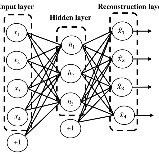
The AE is at the basis a neural network architecture characterized by one hidden layer. It has then three layers, one visible layer of size n, one hidden layer of d nodes and one reconstruction layer with n nodes. Let 𝐱 ∈ ℛ𝑛 be the input vector, 𝐡 ∈ ℛ𝑛 the output of the hidden layer and 𝐱̂ ∈ ℛ𝑛 the output of the AE (reconstruction of 𝐱). d can be inferior or superior to n. In the former case (i.e., d < n), the AE performs feature reduction. In the latter case, however, it performs an over-complete representation [22].
As can be shown in Figure 2-3, the output of the hidden and reconstruction layers can be calculated using the following equations:
𝐡 = 𝑓(𝐖𝐱 + 𝐛) (2.3)
𝐱̂ = 𝑓(𝐖′𝐡 + 𝐛′) (2.4)
Where f(.) is a non-linear activation function, 𝐖 and 𝐛 are the d × n weight matrix and the bias vector of dimension d of the encoding, and 𝐖′ and 𝐛′ are the n × d weight matrix and the bias vector of dimension n of the decoding part.
17
argmin
𝐖,𝐖′,𝐛,𝐛′[ 𝐿(𝐱, 𝐱̂)] (2.5)
The loss function 𝐿(𝐱, 𝐱̂) adopted in this work is the squared error i.e., ‖𝐱 − 𝐱̂‖2. After finding the optimal values of weights and biases, we proceed by removing the last layer (i.e., reconstruction) with its corresponding parameters (𝐖′ and 𝐛′). The layer ‘h’ therefore contains a new feature representation, which can be directly used as inputs into a classifier, or alternatively fed into another higher layer to generate deeper features.
In our case, we add a multinomial logistic regression layer (LRL), known also as softmax classifier, at the end of the encoding part to classify the produced feature representations. The choice of using a LRL is justified by its simplicity and the fact that it does not require any parameter tuning. The LRL is trained by adopting the output of the encoding part (the new feature representation) as input, and the corresponding binary vector as target output.
Figure 2-3: One layer architecture of an AE.
2.4. Feature Fusion
As described so far, three types of features are made use of in this work (HOG, BOW_RGB, and LBP). In order to further improve the classification efficiency, we propose three distinct feature fusion schemes. The first one is a stacked fusion, which consists of extracting the three feature vectors from a given image and then stack them up to form a global feature vector. This latter is injected as an input to an AE topped by a logistic regression layer (LRL). The general diagram of the stacked fusion is observed in Figure 2-4.
h
x
W′ W
Reconstruction
Decoding Feed-backward Encoding Feed-forward
18
Figure 2-4:Diagram of the first fusion strategy (Fusion 1) based on a low-level feature
aggregation.
The second technique is a parallel fusion, as shown in Figure 2-5, which proceeds by feeding each type of feature into an individual AE model, followed by concatenating the learned features to form a single vector. This latter is set as input to another AE model that is connected to a LRL that outputs the final classification results. It is worth to mention that the two blocks composing the autoencoders are trained separately.
Figure 2-5:Diagram of the second fusion strategy (Fusion 2) based on a AE induced-level
aggregation.
The third method is based on a linear sum of the individual decisions of the three types of features. In other words, each feature vector is fed into a separate AE model topped by a LRL. The outputs of each LRL are then averaged to come down to a single real-valued output, which is subsequently thresholded to force its values to either one or zero. Figure 2-6 gives an illustration of the fusion procedure.
Figure 2-6:Diagram of the third fusion strategy (Fusion 3) based on a decision-level
aggregation.
Image
BOW_RGB
HOG
LBP
AE+LRL
Image
BOW_RGB
HOG
LBP
AE
AE
AE
AE+LRL
Image
BOW_RGB
HOG
LBP
AE+LRL
AE+LRL
AE+LRL
19 2.5. Experimental Results
2.5.1 Description of the Wearable System
The developed method is part of a complete prototype which is composed of two parts. The first part is the guidance system, which is responsible of guiding a visually impaired person across an indoor environment from an initial point to a desired destination taking into account the avoidance of the different static and/or dynamic obstacles. The second part is the recognition system, which is meant to describe the indoor site for the blind individual to give him better ability to sense the nearby surrounding environment by providing him with a list of existing objects. Regarding the hardware, the wearable system is composed of a laser range finder for detecting and determining objects distance to the user, a portable CMOS camera model UI-1240LE-C-HQ (IDS Imaging Development Systems, Germany) equipped with a LM4NCL lens (KOWA, Japan), a portable processing unit which can be a laptop, a tablet or a smartphone and a headset for voice input and audio output. The user controls the system by giving vocal instructions (i.e., specific keywords) via a microphone and receives information (e.g., list of objects) vocally synthesized through the earphone. All the hardware is mounted on a wearable jacket as can be seen on Figure 2-7. The design of the entire prototype was performed by taking into consideration the feedbacks we received from VI persons, in particular regarding interfacing and exploitation.
Figure 2-7:View of the wearable prototype with its main components.
2.5.2 Dataset Description
20 end, we have selected the objects deemed to be the most important ones in the considered indoor spaces. Regarding the first dataset, 15 objects were considered as follows: ‘External Window’, ‘Board’, ‘Table’, ‘External Door’, ‘Stair Door’, ‘Access Control Reader’, ‘Office’, ‘Pillar’, ‘Display Screen’, ‘People’, ‘ATM’, ‘Chairs’, ‘Bins’, ‘Internal Door’, and ‘Elevator’. Whereas, for the second dataset, the list was the following: ‘Stairs’, ‘Heater’, ‘Corridor’, ‘Board’, ‘Laboratories’, ‘Bins’, ‘Office’, ‘People’, ‘Pillar’, ‘Elevator’, ‘Reception’, ‘Chairs’, ‘Self Service’, ‘External Door’, and ‘Display Screen’.
2.5.3 Evaluation Metrics and Parameter Setting
For evaluation purposes, we use the well-known sensitivity (SEN) and specificity (SPE) measures:
SEN = 𝑇𝑟𝑢𝑒 𝑃𝑜𝑠𝑖𝑡𝑖𝑣𝑒
𝑇𝑟𝑢𝑒 𝑃𝑜𝑠𝑖𝑡𝑖𝑣𝑒+𝐹𝑎𝑙𝑠𝑒 𝑁𝑒𝑔𝑎𝑡𝑖𝑣𝑒 (2.6)
SPE = 𝑇𝑟𝑢𝑒 𝑁𝑒𝑔𝑎𝑡𝑖𝑣𝑒
𝑇𝑟𝑢𝑒 𝑁𝑒𝑔𝑎𝑡𝑖𝑣𝑒+𝐹𝑎𝑙𝑠𝑒 𝑃𝑜𝑠𝑖𝑡𝑖𝑣𝑒 (2.7)
The sensitivity expresses the classification rate of real positive cases i.e., the efficiency of the algorithm towards detecting existing objects. The specificity, on the other hand, underlines the tendency of the algorithm to detect the true negatives i.e., the non-existing objects. In general, those two quantities reflect opposite measures. In other words, the more the method tends to detect existing objects (high True-Positive which entails higher sensitivity) the more is exposed to make wrong detections (high False-Positive which implies low specificity). In order to make a trade-off between the two measures and to make an adequate comparison of results with respect to the state-of-the-art methods, we propose to further include the average of both:
AVG =SEN+SPE
2 (2.8)
We set the parameters of the three feature extractors as follows.
For HOG features, we set the number of bins to 9 and the size of the cells to 80, which gives a
HOG feature vector of size 1260 (recall that the size of the image is 640 × 480).
Regarding the BOW_RGB, the number of centroids i.e., ‘K’ of the K-means clustering is set to
200, which was observed as the best choice among other options.
For the LBP, we set R = 1, P = 8, and size of the cells = 80, which produces a LBP feature
vector of length 480 bins.
21 exhibit opposite behaviours as the threshold value increases. On average between SEN and SPE, a threshold of 0.3 stands out as the best option, which will be adopted in the remaining experiments.
Figure 2-8:Impact of the threshold value on the classification rates using the three feature types. Upper row for Dataset 1, bottom row for Dataset 2.
2.5.4 Results
We first report the results pointed out by using the three types of features individually. We tried many configuration by changing the size of the hidden layer from 100 to 1000 nodes by a step of 100. Ultimately, 300 nodes turned out to be the best choice for all the features. It can be observed from Table 2-1 that on Dataset 1, the three features perform closely, with a slight improvement being noticed with BoW_RGB. On dataset 2, however, the BoW_RGB outperforms, by far, the remaining two, which was expected beforehand as this dataset particularly manifests richer colour information than the former one. Nevertheless, the yielded rates are quite reasonable taking into account the relatively large number of objects considered in this work, besides other challenges such as scale and orientation changes.
Table 2-1: Obtained recognition results using single features.
Dataset Dataset 1 Dataset 2
Method HOG BoW_RGB LBP HOG BoW_RGB LBP
SEN (%) 76.77 79.77 76.77 72.73 88.64 81.82
SPE (%) 82.16 82.9 80.07 88.67 90.24 86.27
AVG (%) 79.46 81.33 78.42 80.7 89.44 84.04
22 out their best at 500 and 300, respectively. It is to note that all the values within 100–1000 have pointed out nearby performances. The earlier optimal parameters will therefore be adopted in what follows.
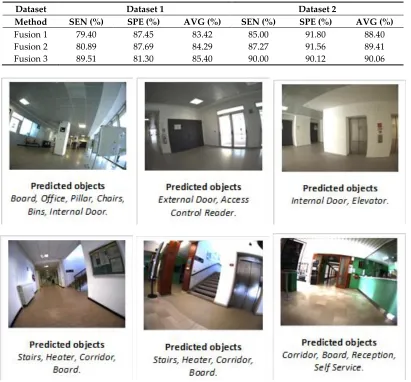
The classification results of the fusion schemes are summarized in Table 2-2 and examples of results obtained for some query images are provided in Figure 2-9 for both datasets. As a first remark, it can be spotted that significant gains have been introduced with respect to using individual features (Table 2-1), which strengthens the assumption that fusing multiple features is likely to be advantageous over individual feature classification scenarios.
Table 2-2: Classification outcomes of all the fusion schemes.
Dataset Dataset 1 Dataset 2
Method SEN (%) SPE (%) AVG (%) SEN (%) SPE (%) AVG (%)
Fusion 1 79.40 87.45 83.42 85.00 91.80 88.40
Fusion 2 80.89 87.69 84.29 87.27 91.56 89.41
Fusion 3 89.51 81.30 85.40 90.00 90.12 90.06
Figure 2-9:Example of results obtained by the proposed multilabeling fusion approach for
both datasets. Upper row for Dataset 1, and lower one for Dataset 2.
23 Dataset 1 and exhibits a better SEN-SPE balance on Dataset 2. As a matter of fact, choosing between SEN or SPE depends upon the application being addressed. In our case, we will privilege SEN as we think it is more important to provide information on the presence of objects (even if it generates some false positives) rather than on the absence of objects. For such purpose, late fusion of individual decisions (i.e., Fusion 3) has proved to be a more efficient option than feature-level fusion (i.e., the first two schemes), with a tendency to score higher or equal SEN rates with respect to SPE.
For the sake of comparison of Fusion 3 strategy with state-of-the-art methods, we considered the contribution made in [15], namely the Semantic Similarity-based Compressed Sensing (SSCS) and the Euclidean Distance-based Compressed Sensing (EDCS) techniques, and also three different pretrained Convolutional Neural Networks (CNNs) which are ResNet [24], GoogLeNet [25] and VDCNs [26]. As shown in Table 2-3, for Dataset 1, our strategy outperforms largely the reference work in [15] with at least 10% of improvement and between 2% to 5% compared to the three pretrained CNNs. Moreover, our method offers the advantage of yielding far higher SEN. Both observations can be traced back to two considerations. On the one hand, the work put forth in [15] makes use of a small-sized dictionary of learning images to represent a given image by means of a compressive sensing-based approach, which might succeed in representing an image that has good matches in the dictionary but may fail when it comes to an (outlier) image that has no match in the dictionary. On the other hand, the proposed approach proceeds by extracting robust features capable to capture different variations across the images, followed by a customized feature learning step that furthers their discrimination capacity, which is ultimately reflected on higher classification rates as the results tell. The same observations apply for Dataset 2 as seen in Table 2-4.
Table 2-3: Comparison of classification rates on Dataset 1.
Method SEN (%) SPE (%) AVG (%)
SSCS 79.77 66.54 73.15
EDCS 69.66 80.19 74.92
ResNet 66.29 94.46 80.38
GoogLeNet 67.04 94.22 80.63
VDCNs 71.91 94.46 83.19
Ours 89.51 81.3 85.40
Table 2-4: Comparison of classification rates on Dataset 2.
Method SEN (%) SPE (%) AVG (%)
SSCS 75 74.09 74.54
EDCS 70 90.12 80.06
ResNet 68.18 96.75 82.46
GoogLeNet 72.27 97.11 84.69
VDCNs 81.82 96.39 89.10
Ours 90.00 90.12 90.06
24 10% of the original size. The classification results in terms of AVG accuracy are shown in Table 2-5 and Table 2-6 for both datasets, respectively. It can be observed that the accuracy does not manifest drastic changes as the image size drops. In fact, there are instances where the smallest resolutions introduce slight improvements, which we believe can be interpreted by the fact that, in many images, there are large background surfaces (e.g., walls) that have usually uniform colours and textures, which may not be really useful as salient visual properties by which the images can be discriminated, reducing the image size thereby reduces the size occupied by those backgrounds, which may either maintain or even raise the classification performance.
Table 2-5: Comparison of classification rates on Dataset 1 under different resolutions.
Method 100% 50% 20% 10%
SSCS 73.15 73.34 74.52 74.51
EDCS 74.92 74.74 75.11 75.43
ResNet 80.38 79.88 79.32 78.76
GoogLeNet 80.63 81.63 82.52 79.02
VDCNs 83.19 83.37 84.50 84.57
Ours 85.40 86.02 86.14 86.63
Table 2-6: Comparison of classification rates on Dataset 2 under different resolutions.
Method 100% 50% 20% 10%
SSCS 74.54 74.54 73.91 74.48
EDCS 80.06 80.06 79.30 78.60
ResNet 82.46 82.40 84.69 87.13
GoogLeNet 84.69 84.69 84.74 84.12
VDCNs 89.10 88.71 87.80 88.13
Ours 90.06 90.34 90.03 90.69
Besides the classification rates, another important performance parameter is the runtime. For the proposed method, the runtime includes the feature extraction, the prediction and the fusion times. We provide the average processing time per image for both datasets in Table 2-7 and Table 2-8, from which it can be seen that, as expected, the runtime decreases with the image size, with our method being at least four times faster than the best runtime (GoogLeNet) provided by methods of reference. Particularly, 22 milliseconds per image is a very promising time span provided that fifteen objects are targeted in this work. Such processing time is based on a Matlab R2016b implementation, which is subject to be drastically reduced under for instance a C++ implementation. It is also worth mentioning that the number of objects in our work does not impact on the classification process.
Table 2-7: Comparison of average runtime per image on Dataset 1 under different resolutions.
Method 100% 50% 20% 10%
SSCS 2.16 1.42 1.22 1.17
EDCS 2.44 1.41 1.1 1.08
ResNet 0.136 0.132 0.131 0.131
GoogLeNet 0.100 0.098 0.096 0.093
VDCNs 0.300 0.295 0.291 0.288
25 Table 2-8: Comparison of average runtime per image on Dataset 2 under different resolutions.
Method 100% 50% 20% 10%
SSCS 2.66 1.53 1.21 1.17
EDCS 2.69 1.54 1.23 1.2
ResNet 0.136 0.132 0.131 0.131
GoogLeNet 0.100 0.098 0.096 0.093
VDCNs 0.300 0.295 0.291 0.288
Ours 1.230 0.200 0.048 0.022
2.6. Conclusions
This chapter presented a scene description (via image multilabeling) methodology meant to assist visually impaired people to conceive a more accurate perception about their surrounding objects in indoor spaces. The idea of the proposed method is promoted around detecting multiple objects at once within a possible short runtime. A key-determinant of our image multilabeling scheme is that the number objects is independent of the classification system, which entails the property of detecting as many objects as desired (depending on the offline setup to be customized by the user) within the same amount of time which amounts for much less than a second in our work.
The multilabeling algorithm exploits feature learning concept by means of an AutoEncoder neural network, which amply demonstrated a significant potential in generating discriminative image representations.
Pros: In the literature, there exist several multi-object recognition methods (but not in the context of visually impaired rehabilitation). Those methods, may show interesting recognition efficiency, but they are dependent on the number of objects considered. By contrast, our method as hinted earlier, does not, which renders it much faster yet more reliable if considered in real-time scenarios. The earlier two points are technically verified in [15], where it was concluded that coarse image description is more adequate in this sense.