International Doctorate School in Information and Communication Technologies
DIT - University of Trento
Modeling and Querying Data Series and
Data Streams with Uncertainty
Michele Dallachiesa
Advisor:
Prof. Themis Palpanas
Universit`a degli Studi di Trento
Many real applications consume data that is intrinsically uncertain and error-prone. An uncertain data series is a series whose point values are uncertain. An uncertain data stream is a data stream whose tuples are existentially uncertain and/or have an uncertain value. Typical sources of uncertainty in data series and data streams include sensor data, data synopses, privacy-preserving transformations and forecasting models. In this thesis, we focus on the following three problems: (1) the formulation and the evaluation of similarity search queries in uncertain data series; (2) the evaluation of nearest neighbor search queries in uncertain data series; (3) the adaptation of sliding windows in uncertain data stream processing to accommodate existential and value uncertainty. We demonstrate ex-perimentally that the correlation among neighboring time-stamps in data series can be leveraged to increase the accuracy of the results. We fur-ther show that the ”possible world” semantics can be used as underlying uncertainty model to formulate nearest neighbor queries that can be eval-uated efficiently. Finally, we discuss the relation between existential and value uncertainty in data stream applications, and verify experimentally our proposal of uncertain sliding windows.
Keywords
1 Introduction 1
1.1 Motivating Scenarios . . . 2
1.2 Modeling and Querying Uncertain Data Series . . . 5
1.2.1 Contributions . . . 6
1.3 Top-k Nearest Neighbor Search in Uncertain Data Series . 6 1.3.1 Contributions . . . 7
1.4 Management of Sliding Windows in Uncertain Data Streams 8 1.4.1 Contributions . . . 9
1.5 Structure of the Thesis . . . 10
2 Related Work 11 2.1 Nearest Neighbor Queries . . . 12
2.2 Uncertain Data Streams . . . 15
3 Preliminaries 21 4 Uncertain Time-Series Similarity: Return to the Basics 23 4.1 Similarity Matching for Uncertain Time Series . . . 24
4.1.1 MUNICH . . . 25
4.1.2 PROUD . . . 27
4.1.3 DUST . . . 29
4.2.2 Type of Distance Measures . . . 32
4.2.3 Type of Similarity Queries . . . 32
4.3 Comparative Study . . . 33
4.3.1 Experimental Setup . . . 33
4.3.2 Quality Performance . . . 36
4.3.3 Time Performance . . . 41
4.4 Moving Average for Uncertain Time Series . . . 43
4.4.1 Neighborhood-Aware Models . . . 44
4.4.2 Performance . . . 45
4.5 Discussion . . . 48
4.6 Summary . . . 51
5 Top-k Nearest Neighbor Search for Uncertain Data Series 53 5.1 Preliminaries . . . 54
5.1.1 Problem Statement . . . 57
5.2 Baseline Algorithm . . . 58
5.2.1 Complexity Analysis . . . 59
5.3 Proposed Approach . . . 60
5.3.1 Bounding the PNN Probability Estimates . . . 60
5.3.2 The Holistic-PkNN Algorithm . . . 63
5.3.3 Tightening the PNN Bounds . . . 66
5.3.4 Managing the Distance Partitions . . . 73
5.4 Indexing Uncertain Data Series . . . 77
5.4.1 Bulk-loading Algorithm . . . 78
5.4.2 Pruning the Search Space . . . 79
5.5 Extensions . . . 80
5.6 Experimental results . . . 81
5.6.3 Quality Results . . . 85
5.6.4 Time performance . . . 85
5.7 Summary . . . 96
6 Sliding Windows over Uncertain Data Streams 99 6.1 Uncertain data streams . . . 101
6.1.1 Preliminaries . . . 101
6.1.2 From value to existential uncertainty . . . 102
6.1.3 From existential to value uncertainty . . . 103
6.2 Uncertain Sliding Windows . . . 104
6.2.1 Modeling uncertain sliding windows . . . 105
6.2.2 Processing uncertain sliding windows . . . 107
6.2.3 The Poisson-binomial distribution . . . 109
6.2.4 Efficient approximations of the Poisson-binomial dis-tribution . . . 111
6.3 Adapting stream operators to handle data uncertainty . . 112
6.4 Efficient similarity join processing . . . 115
6.4.1 Upper-bounding the match probability . . . 116
6.4.2 Pruning the similarity search space . . . 117
6.5 Experimental evaluation . . . 120
6.5.1 Datasets . . . 121
6.5.2 Poisson-binomial distribution approximations . . . 122
6.5.3 Uncertain sliding windows for sum aggregation . . . 127
6.5.4 Uncertain sliding windows for similarity join . . . . 128
6.6 Extensions . . . 137
6.6.1 Other sliding window policies . . . 137
6.6.2 Integration into System S . . . 138
5.1 Notation used in this chapter. . . 57 5.2 Experiment parameter configuration ranges. Default values
are indicated in bold. . . 85
6.1 Symbols used in the chapter and their explanations. . . 105 6.2 Experiment parameter configuration ranges. Default values
4.1 Example of uncertain time series X = {x1, ..., xn} modeled
by means of pdf estimation. . . 26
4.2 Example of uncertain time series X = {x1, ..., xn} modeled
by means of repeated observations. . . 26
4.3 The probabilistic distance model. . . 28
4.4 F1 score for MUNICH, PROUD, DUST and Euclidean on
Gun Point truncated dataset, when varying the error stan-dard deviation: normal error distribution (left), uniform
(center), exponential (right). . . 38
4.5 F1 score for PROUD, DUST and Euclidean, averaged over
all datasets, when varying the error standard deviation: nor-mal error distribution (left), uniform (center), exponential
(right). . . 38
4.6 Precision and recall for PROUD, averaged over all datasets,
when varying error standard deviation and error distribution. 39
4.7 Precision and recall for DUST, averaged over all datasets,
when varying error standard deviation and error distribution. 40
4.8 F1 score for PROUD, DUST, and Euclidean on all the datasets
with mixed error distribution (normal), 20% with standard
nential), 20% with standard deviation 1.0, and 80% with
standard deviation 0.4. . . 41
4.10 F1 score for PROUD, DUST, and Euclidean on all the datasets
with mixed error distribution: normal, with standard
devi-ation erroneously reported as constant 0.7. . . 42
4.11 Average time per query for PROUD, DUST, and Euclidean, averaged over all datasets, when varying the error standard
deviation with normal error distribution. . . 43
4.12 Average time per query for PROUD, DUST, and Euclidean, averaged over all datasets, when varying the time series
length with normal error distribution. . . 43
4.13 F1 score varying the window size, w, for UMA and UEMA
(with λ = 0.1,1). . . 46
4.14 F1 score varying the decaying factor, λ, for UEMA (for w =
5,10). . . 47
4.15 F1 score for all datasets and mixed error distribution: uni-form with 20% standard deviation 1.0, and 80% standard
deviation 0.4. . . 49
4.16 F1 score for all datasets and mixed error distribution: nor-mal with 20% standard deviation 1.0, and 80% with
stan-dard deviation 0.4. . . 49
4.17 F1 score for all datasets and mixed error distribution: ex-ponential with 20% standard deviation 1.0, and 80% with
value-uncertainty model. Graph (b) shows the uncertain series Xi introduced in graph (a), modeled using the
series-uncertainty model with samples Xi1 and Xi2. Graph (c)
shows an uncertain series Xj that is distinguishable from
uncertain series Xi under the series-uncertainty model but
not under the value-uncertainty model. . . 55 5.2 Example of valid distance partition instantiationsSimin,Simid
and Smax
i representing the distance samples in Dist(Q, Xi). 61
5.3 Graph (a) shows an example of critical region R with over-lapping PNN probability bounds B3 and B2. Graph (b)
reports an example of empty critical region R. . . 64 5.4 Graph (a ) shows the critical region R, where B2 is a left
crosser. Graph (b) shows the critical region R, where B1 is
a double crosser and B2 is a left crosser. . . 69
5.5 Graph (a) shows the distance partitions Si and graph (b)
reports their respective PNN bounds Bi. . . 70
5.6 Example of uncertain series envelope. . . 74 5.7 Example of metric distance bounds. . . 75 5.8 Accuracy when varying the perturbation standard deviation
σ using the NN classifiers based on the Top-k-PN N(D, Q, k)
and Euclidean-Avg algorithms. . . 86
5.9 Ratio of retained candidates when varying the number of uncertain series samples m for distance partitions initialized
with spatial, metric and exact distance bounds, respectively. 88
5.10 Ratio of retained candidates when varying the perturbation standard deviation σ for distance partitions initialized with
metric and exact distance bounds, respectively. . . 88
5.12 Ratio of retained candidates when varying the number of pivots for the metric distance bounds using different pivot
selection strategies random, max-dist and k-means. . . 89
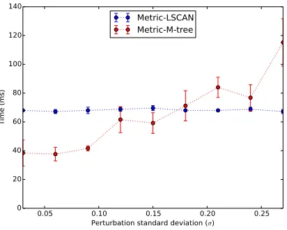
5.13 Time performance when varying perturbation standard de-viation for linear-scan and M-tree techniques for distance
partitions initialized using metric distance bounds. . . 90
5.14 Time performance when varying the number of samples m
for distance partitions initialized with spatial, metric and
exact distance bounds, respectively. . . 91
5.15 Time performance when varying the perturbation standard deviation σ for distance partitions initialized with spatial,
metric and exact distance bounds, respectively. . . 91
5.16 Time performance when varying the number of uncertain se-ries N for distance partitions initialized with spatial, metric
and exact distance bounds, respectively. . . 91
5.17 Time performance when varying number of samples m for
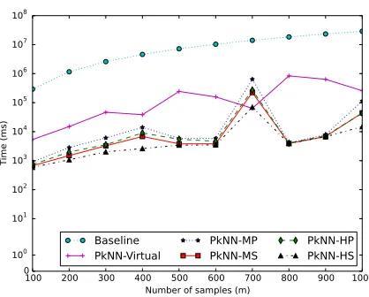
Baseline and Holistic-PkNN algorithms. . . 93
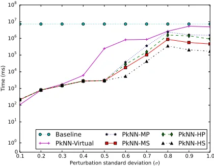
5.18 Time performance when varying the perturbation standard
deviation σ for Baseline and Holistic-PkNN algorithms. . 94
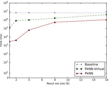
5.19 Time performance when varying the number k of retrieved uncertain series for theBaseline,Holistic-PkNNand
Holistic-PkNN-Virtual algorithms. . . 95
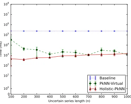
5.20 Time performance when varying the uncertain series length
nfor theBaseline,Holistic-PkNNandHolistic-PkNN-Virtual
uncertain series length n for the Holistic-PkNN algorithm. 97
5.22 Time performance for different levels of perturbation stan-dard deviation σ when varying the number of uncertain
se-ries N using the Holistic-PkNN algorithm. . . 98
5.23 Time performance for different configurations of the number of uncertain series samples m when varying the number of
uncertain series N using the Holistic-PkNN algorithm. . . 98
6.1 Example of an uncertain data stream, where uncertainty is modeled by repeated weighted measurements and tuples are 1-dimensional points. Weights are encoded using
trans-parency, i.e., lighter points occur with lower probability. . . 102
6.2 Example of an uncertain sliding window. Bounding inter-vals drawn using dashed lines represent the sliding window content, whereas light colored bars represent existentially
uncertain tuples. . . 104
6.3 Example of a similarity join between certain data streams. Interval bar displays tuples in W(T, w) that are similar to
sη+1 based on the distance threshold ǫ. Blue (dark) and red
(light) dots represent the values of the two streams to be
joined. . . 114
6.4 RMSE of different Poisson-binomial approximations for dif-ferent window sizes and with existential uncertainty distri-bution standard deviation set to 0.1 (Normal distribution). The approximation with lowest error is the Refined Normal, independent of the distribution used for assigning tuple exis-tential uncertainties. The figure also shows the low precision
provide the lowest cost. . . 125
6.6 F1 score for the similarity join operator when comparing the use of CDF approximations. Join using Normal & Refined Normal approximations provide results very similar to an
exact solution. . . 125
6.7 Precision for the similarity join operator when using CDF
approximations. . . 126
6.8 Recall for the similarity join operator when using CDF
ap-proximations. . . 126
6.9 Absolute percentage change of the output tuple values when substituting a regular sliding window W(V, w) with an un-certain sliding window W(V, w, α) for different configura-tions of window size w when varying the α probabilistic
threshold. . . 128
6.10 Actual size of uncertain sliding windows when varying the existential uncertainty standard deviations (σ). Memory footprint increases as the existential uncertainty standard
deviation increases. . . 130
6.11 Actual size of uncertain sliding windows when varying the probabilistic threshold α and the existential uncertainty σ. Window size is more sensitive to σ than α. It also presents
a steep increase as α approaches to 1. . . 131
6.12 Ratio of uncertain sliding window lengths maintained by eviction policiesuncert-evict-beta anduncert-evict when vary-ing the α probabilistic threshold. uncert-evict-beta policy
ferent window sizes. . . 134 6.14 Performance of pruning strategies when varying the number
of samples. . . 135 6.15 Average time performance of different pruning strategies
Introduction
In recent years, the database and data mining community has investi-gated extensively the problem of modeling and querying uncertain data [4, 33], and several probabilistic database systems have been proposed [41, 7, 32, 10, 81]. Uncertainty can occur for different reasons, includ-ing the inherent imprecision in the sensor observations, approximations introduced by summarization techniques, privacy-preserving transforma-tions of sensitive records, applicatransforma-tions in data integration and predictive models whose output is intrinsically uncertain.
Uncertain data poses significant challenges to data management. First, uncertainty needs to be modeled and represented. Each model is a trade-off between its ability to represent the complex underlying dependencies in uncertain data and its tractability and efficiency in a database sys-tem. Second, the formulation of traditional database queries and mining tasks must be revisited to accommodate the differences in the data repre-sentation, typically introducing probabilistic thresholds and other quality guarantees.
a novel model based on the moving average; (2) the efficient evaluation of nearest neighbor search queries in uncertain data series, unifying and extending prior works in the field; (3) the adaptation of sliding windows in uncertain data streams to accommodate the existential uncertainty of the processed tuples by introducing the novel concept of uncertain sliding windows.
In the next section, we describe some use cases, where modeling ex-plicitly the uncertainty of the underlying data is beneficial in real-world applications, and we then introduce the three problems that we study in this thesis summarizing our contributions.
1.1
Motivating Scenarios
The fast growing availability of sensor measurements is fueled by the raise of wearable devices and connected devices, as well as more traditional data sources such as meteorology, astronomy, computer vision and indus-trial monitoring. Applications in the above domains usually organize these sequential measurements into time series, i.e., sequences of data points or-dered along the temporal dimension, making time series a data type of particular importance. Several studies have recently focused on the prob-lems of processing and mining time series with incomplete, imprecise and even misleading measurements [21, 58, 85, 86, 91]. Some examples in real scenarios are listed below:
geologic observing systems, pollution management in urban settings, and application of water and fertilizers in precision agriculture. In transportation, sensor networks are employed to monitor weather and traffic conditions, and increase driving safety [75]. However, sensor data is inherently imprecise. Measurements are sampled from error-prone equipment [21], whose accuracy depends heavily on environ-mental conditions such as humidity and temperature. Furthermore, errors can be introduced during the processing and the wireless trans-mission in sensor networks. Repeated measurements can be obtained from multiple sensors to determine an aggregate value with higher confidence.
• Personal information contributed by individuals and corporations is steadily increasing, and there is a parallel growing interest in applica-tions that can be developed by mining these datasets, such as location-based services and social network applications. In these applications privacy is a major concern, addressed by various privacy-preserving transforms [3, 40, 73], which introduce data uncertainty. The data can still be mined and queried, but it requires a re-design of the existing methods in order to address this uncertainty.
• Forecasting models are used to predict future events such as weather conditions and market trends. Nevertheless, predictive models are also used by researchers as a convenient language to encode the complex semantics of the studied phenomena in natural sciences and other disciplines. Uncertainty is an inherent property of such models, that can be regarded as a measure of the goodness of the model itself.
uncertain time series.
In other applications, the sensor measurements arrive continuously and are organized as data streams. Streams of sensor measurements are widely used as inputs of real-time analytics monitoring and applications. The strong demand for applications that continuously monitor the occurrence of interesting events (e.g., road-tunnel management [75] and health moni-toring [84]) has driven the research in data stream processing systems [2, 43, 94]. In many of these application domains, the data sources avail-able for processing can be considered uncertain. Some examples in real scenarios are listed below:
• In offshore drilling operations [71], data sources can be inaccurate, and pose significant challenges to the monitoring systems. Oil companies want to avoid shutting down operations as much as possible. To detect when operations must indeed be stopped, such companies deploy mon-itoring systems to collect real-time sensor measurements, such as pres-sure, temperature, and mass transport along the well path. Streaming applications process the sensor data through prediction models, which generate alarms and warnings with an associated confidence.
inaccurate data in such scenarios.
In the remainder of this Chapter we introduce the open problems and summarize our contributions.
1.2
Modeling and Querying Uncertain Data Series
In this thesis we consider the problem of evaluating similarity range queries in uncertain data series. A range query returns a set of uncertain series whose distance to the query is lower than a predefined threshold with a known confidence level. We note that two uncertain series may be very similar with low probability. At the same time, they can be very differ-ent with high probability. The semantics of similarity in uncertain data involves distance and probabilistic thresholds. The uncertainty model and the similarity semantics affect significantly the result set.
top of it [89, 63, 66].
1.2.1 Contributions
Our evaluation reveals the effectiveness of the techniques that have been proposed in the literature under different scenarios. In the experiments, we stress-test the different techniques both in situations for which they were designed, as well as in situations that fall outside their normal oper-ation (e.g., unknown distributions of the uncertain values). In the latter case, we wish to establish how strong the assumptions behind the design principles of each technique are, and to what extent these techniques can produce reliable and stable results, when these assumptions no longer hold. We note that such situations do arise in practice, where it is not always possible to know the exact data characteristics of the uncertain time se-ries. Furthermore, we describe additional similarity measures for uncertain time series, inspired by the moving average, namely Uncertain Moving Av-erage (UMA), and Uncertain Exponential Moving AvAv-erage (UEMA). Even though these similarity measures are very simple, previous studies had not considered them. However, the experimental evaluation shows that they perform better than the more sophisticated techniques that have been pro-posed in the literature. We observe that UMA and UEMA incorporate some of the information inherent in the sequence of points in the time series, thus, taking a step back from the independence assumption of the other techniques.
1.3
Top-
k
Nearest Neighbor Search in Uncertain Data
Series
en-gines, and location-based services. A nearest neighbor search returns the uncertain series in the dataset whose distance to the query is the small-est one. A top-k nearest neighbor search returns the k closest uncertain series to the query. Similarly to range queries, the semantics depend on the adopted uncertainty model and the formulation of nearest neighbor in uncertain data.
The problem of identifying the top-k nearest neighbors has been widely studied in traditional database systems [48]. Its popularity is largely due to the simplicity of tuning the k parameter in contrast to other queries such as similarity search, where a distance threshold has to be provided. Similarly, the evaluation of top-k nearest queries has received considerable attention in probabilistic databases [26, 76, 56, 83, 16, 62, 28]. The high di-mensionality and the highly correlated dimensions of uncertain data series pose significant new challenges to the efficient evaluation of top-k nearest neighbor searches in uncertain series.
1.3.1 Contributions
1.4
Management of Sliding Windows in Uncertain
Data Streams
An uncertain data stream is a data stream whose tuples are existentially uncertain. The value assigned to each tuple is uncertain. In many ap-plications, data streams are processed through sliding windows. A sliding window of size w identifies the set of the mostw recent tuples and advances when a new tuple comes in. The semantics of sliding windows need to be revisited to accommodate the existential uncertainty of the stream tuples. In this study, we investigate the adaptation of sliding windows to uncertain data streams.
Current research in processing uncertain data streams focuses mostly on the development of specific stream operators (e.g., joins [57, 61] and aggregates [49]) and specific queries (e.g., top-k [51, 97] and clustering [5]) that can operate in the presence of value uncertainty. These works are not designed with the integration into current general-purpose stream pro-cessing engines in mind. This is because they ignore the challenges arising from operator composition (different operators are connected to form an operator graph), which is a common development paradigm when writing streaming queries [2, 46, 70]. One such challenge is to consider streams with existential uncertainty. Existential uncertainty arises when applying certain transformations to streams with value uncertainty. For example, tuples may be generated when an event is triggered. If the event is uncer-tain, then the new tuple may not exist in some possible world instantiation. As a result, the regular sliding windows can over-estimate the window size, not considering the possibility that some data values do not exist in the window. Processing streams with existential uncertainty has an impact on
window management, which is one of the basic building blocks of stream
algorithms that require access to the most recent history of a stream, such as aggregations, joins, and sorts. Windows can have different behaviors (e.g., tumbling and sliding) and configurations (e.g., size). Window sizes can be defined based on time (e.g, all tuples collected in the last x sec-onds) or based on a count (e.g., last x tuples). Count-based windows are especially useful for coping with the unpredictable incoming rate of data streams. By limiting the size of the windows, developers can ensure that the memory consumed by the operator can be bounded. In existentially certain streams, establishing the boundaries of a window is trivial, since every tuple processed is guaranteed to be present in the stream. However, how should one manage such windows considering that in existentially un-certain streams it is not guaranteed that a tuple is indeed present in a given window bound? We note that the characteristics of the data streams may vary over time and a constant, larger window size may lead to overestimates of the desired window size, eventually causing undesired and unexpected effects. In this study, we investigate this problem.
1.4.1 Contributions
1.5
Structure of the Thesis
The thesis is structured as follows. In Chapter 2, we review the state of the art and introduce the preliminaries in Chapter 3. In Chapter 4, we compare prior studies to evaluate similarity range queries in uncertain data series and propose novel models based on the moving average. In Chapter 5, we present our algorithms for the efficient evaluation of top-k
Related Work
The problem of modeling, querying and mining uncertain data has been investigated extensively in recent years [4, 33]. A comprehensive review of the models and algorithms introduced by the database community can be found in [6]. Several database systems supporting uncertain data have been proposed, such as Conquer [41], Trio [7], MistiQ [32], MayMBS [10] and Orion [81].
The ”possible worlds” model formalizes uncertainty by defining the space of the possible instantiations of the database. Instantiations must be consistent with the semantics of the data. For example, in a spatio-temporal database there may be two distinct possible trajectories repre-senting the uncertain trajectory of a moving object, but an object cannot be in two different locations at the same time. The main advantage of the ”possible worlds” model is that the formulations of the queries originally designed for certain data can be directly applied on each possible instan-tiation. Many different alternatives have then been proposed to aggregate the results across the different instantiations.
leverage its simplicity: The tuple- and the attribute-uncertainty models [50, 6]. In the attribute-uncertainty model, the uncertain tuple is repre-sented by means of multiple samples drawn from its Probability Density Function (PDF). In contrast, in the tuple-uncertainty model the value of the tuple is fixed but the tuple itself may not exist with some probability. In the context of time series databases, a series can be formalized as a point in a high-dimensional space with correlated dimensions. An uncer-tain series can then be represented by enumerating its possible instantia-tions under the ”possible world” semantics. Prior works on uncertain time series [79, 95, 11] introduce the additional assumption of independence across different timestamps. Nevertheless, temporal correlation is a well known property of time series data and ignoring it may lead to erroneous results.
We proceed reviewing prior studies focusing on the evaluation of top-k
nearest neighbor searches in uncertain data.
2.1
Nearest Neighbor Queries
The evaluation of Top-k nearest neighbor queries on uncertain data is a well recognized problem, that can be tracked back to the seminal work of Cheng et al. [26]. Subsequently many different formulations of ”nearest neighbor” in uncertain data have been proposed. A detailed review of the state of the art can be found in [50].
of this four-step approach can be found in nearly all the subsequent studies tackling the same problems.
In [76] Re et al. proposed the Multi-Simulation (MS) algorithm to discern the Top-K most probable NN objects by running in parallel several Monte-Carlo simulations. The objects that cannot be safely added to the result set or that cannot be discarded are identified by using the notion of critical region. The critical region is a region in the probability space. Each object is represented by its probability interval of being the NN. The objects having their probability intervals overlapping with the critical region are selected for another simulation step until convergence (i.e., the critical region is empty). In contrary to what considered in our study, the NN probability bounds for different objects are not correlated.
In [56] Kriegel et al. studied the efficient evaluation of probabilistic NN queries as formulated in [26] where each uncertain object is represented by a set of possible instantiations.The samples of each object are clustered using the k-means algorithm, thus obtaining a set of bounding regions that represent the identified clusters. The clusters are then indexed using an R-tree. Similarly to [76], Monte-Carlo simulations are efficiently evaluated on the constructed R-tree to determine the NN probability estimates.
In [83] Soliman et al. introduced the U-Top-k and U-kRanks queries and algorithms for their efficient evaluation on traditional DBMS. Objects are retrieved in minimum-distance order relying on the underlying DBMS capabilities and candidate result sets are then determined. The search terminates when any non-retrieved object can be safely pruned.
retrieved objects are represented by spatial regions that bound their uncer-tain location. When the bounding regions overlap, they are partitioned to obtain a more fine-grained representation of the object uncertainties. The algorithm terminates when the ”virtual” object (and thus all non-retrieved objects) can be safely pruned and the bounding regions of the objects have been sufficiently refined to discriminate their NN probabilities.
In [62] Lian et al. studied the efficient evaluation of pRank queries (equivalent to U-kRanks queries [83]). The uncertain objects are bounded to spatial regions and indexed using an R-tree. The index is then used to prune the candidate objects that have zero probability of being part of the result set. Pre-computed values of the inverse of the Cumulative Density Function (CDF) of the objects are then used to determine their Top-K-NN probability bounds. Eventually the object probabilities are estimated using exact numerical methods if the Top-K-NN probability bounds are not enough tight to discriminate the objects in the result set with enough accuracy.
In [28] Cheng et al. introduced the concept of probabilistic verifiers
to evaluate efficiently the approximate answer to Top-K-NN queries as formulated in [26]. Similarly to prior works, spatial regions bounding the uncertain objects are indexed using an R-tree to perform spatial pruning. Histograms representing the object Probability Density Functions (PDFs) are then used to determine the NN probability bounds. If further tightening of the probability bounds is required, histogram bins are approximated to point values until convergence.
Ide-ally a NN search on a spatial index will return only the NN point. In practice a larger number of points is returned because their index repre-sentations are not enough accurate. The ratio of pruned candidates is a measure of the dataset indexability and serve as a measure of the good-ness of the index structure. Minimum Bounding Rectangles (MBRs) are a popular representation of bounding regions in spatial indexes. Envelopes are their natural extension to data series. An envelope is a pair of series s.t. their value at each time-stamp t represents respectively the minimum and maximum values of the represented series at time-stamp t. Index structures and multi-resolution representations of data series that rely on envelope synopses include iSAX [20] and Haar wavelet transforms [22]. Recently, a new line of research focused on indexing uncertain objects in metric spaces [9]. In [9] Angiulli et al. introduced the UP-Index to sup-port the efficient evaluation of range queries by maintaining statistics on the distance distribution between the indexed objects and a set of pivot objects. These statistics are then used at query time to prune the search space using probability bounds based on the reverse triangular inequal-ity. The algorithm cannot be easily adapted to evaluate Top-K-NN queries since it doesn’t model the relationships between the indexed objects. At best of our knowledge, no prior works considered the problem of evaluating Top-K-NN queries for uncertain data in metric spaces.
2.2
Uncertain Data Streams
In the last decade, several database and stream processing systems with support for uncertainty have been proposed [12, 36, 53, 82, 31, 51, 90, 91], eventually leading to two emerging tuple models.
The x-tuple model [12] represents uncertain tuples by multiple
prob-abilities do not sum up to one, there exists possible instantiations of the uncertain stream where the tuple does not exist. Uncertain tuples are processed according to the possible worlds semantics [44].
In the attribute model [36, 82], uncertainty is more fine-grained and it refers to single tuple attributes. An uncertain attribute is represented by a random variable s.t. its distribution is assumed to be known. The distribution may be continuous or discrete, and it is fully described by its Probability Density Function (PDF). The baseline formalization of this model fails to capture correlations among attributes. Extensions have been proposed to address this limitation [82].
In this study we adopt the x-tuple model. This choice is motivated by the following observations. First, it can capture correlations among attributes without considering more complex extensions (i.e., making ex-plicit the tuple distribution by means of a set of drawn samples). Second, it supports both value uncertainty and existential uncertainty of tuples. Third, real-world uncertain data is often provided by means of discrete samples drawn from unknown distributions. Fourth, possible worlds se-mantics provide an intuitive bridge between sese-mantics of stream operators in certain data streams and their respective adaptations for uncertain data streams. Last but not the least, we observe that applying stream operators to uncertain streams can lead to complex distributions that do not have a closed form. This requires capturing data stream dynamics by reasoning on complex distributions, relying on methods like Monte Carlo estimation, which usually cannot be performed efficiently.
In what follows, we give an overview of relevant work in the literature on processing data streams with uncertainty, adopting the uncertainty models described above.
probabilistic pruning are used to filter the search space efficiently. The two data streams are processed through a pair of sliding windows, and candi-date matches are identified by the sliding window contents. This study is orthogonal to our proposal, and it is used to evaluate the effectiveness of our techniques.
Diao et al. [36] propose a data stream processing system that supports uncertainty modeled by continuous random variables. It also contributes two real-world use cases, namely object tracking on RFID networks and monitoring of hazardous weather conditions.
R´e et al. [77] propose an event processing system for probabilistic event streams by using Markovian models to infer hidden (possibly correlated) variables, e.g., a person’s location from RFID readings. It is worth noting that this system can produce output events that are existentially uncertain. Dallachiesa et al. [31] perform an extensive experimental and analyt-ical comparison of methods for answering similarity matching queries on uncertain time series.
In [30], an augmented R-tree indexes a dataset of spatial points with existential uncertainty. The authors represent existential uncertainty by independent probability values associated to the indexed points. Inter-mediate nodes maintain aggregate statistics, summarizing the existential probabilities of the indexed points in their subtrees. Augmented R-trees support probabilistic range queries, reporting only matching points with existential probabilities higher than a user-defined threshold.
In [60], the authors consider the problem of identifying frequent itemsets in uncertain data streams. Uncertain data streams are processed through a sliding window containing a fixed number of batches (each batch con-tains a fixed number of transactions). The existential probability of each transaction is represented by an independent probability value. Also in this study, the window size is fixed and it does not change over time.
Zhang et al. [98] propose an efficient method to maintain skylines over uncertain data streams. A skyline is a set of items s.t. they are not dominated by any other item. An item i dominates item j if it is “better” than j in at least one tuple attribute and not “worse” than j in all the other tuple attributes. The definitions of “better” and “worse” are domain-specific. The skyline is maintained over a sliding window. The window size is fixed. The probability for each item to belong to the skyline is then estimated by enumerating all the possible worlds. Only skyline items with probability higher than a user-defined thresholds are reported.
In the aforementioned papers, the occurrence probabilities of items in a data stream do not affect the sliding window size. The window size is fixed and does not depend on data uncertainty. In our study, we extend the semantics of sliding window query processing by referring to the window size as the number of truly existing tuples in the uncertain data stream. Our contribution is a basic building block for processing sliding windows on uncertain data streams, and it is orthogonal to past studies. As shown in Section 6.4, previous works on streaming operations with sliding windows can be easily adapted to accommodate our extensions.
Preliminaries
In this section, we overview the definitions of uncertain data series and uncertain data stream.
A data series1 S is an ordered sequence of n real valued numbers S =
S[t], 1 ≤ t ≤ n. For ease of exposition, we refer to the ith point of series S also as si. Where not specified otherwise, we assume normalized
time series with zero mean and unit variance. Notice that normalization is a preprocessing step that requires particular care to address specific situations [64]. An uncertain data series X is a data series whose values at each time-stamp are uncertain. We adopt the attribute-uncertainty model under the ”possible world” semantics to represent uncertain series. Under the attribute-uncertainty model, the series always exists but its value is uncertain. The value uncertainty along the series is represented by means of repeated instantiations, i.e., samples.
An instantiation can be represented by a real-valued sample drawn in-dependently from the value distribution at every time-stamp or by a series sample drawn from the full-joint distribution of the uncertain series. The properties and the implications of these two alternative models are dis-cussed in Chapter 5.
A data stream S is a sequence of tuples si, where 0 ≤i ≤ η and η ∈ N,
1
where η is the index of the most recent tuple received from stream S. We refer to i as the index of a tuple in a stream. Without loss of generality, a tuple si is a d−dimensional real-valued point 2. We define a subsequence
of stream S as S[i,j] = hsi, . . . , sji. We define a count-based sliding window
W(S, w) as the subsequence S[η−w+1,η], where w ∈ N indicates the size of
the window. When not implicit from the context, we refer to data streams without uncertainty as certain data streams.
An uncertain data stream U is a sequence of uncertain tuples ui, where
0 ≤ i ≤ η and η ∈ N. Tuple ui is represented by a set of l possible
mate-rializations, i.e., ui = {ui,1, . . . , ui,l}. If |ui| > 1, then the tuple has value
uncertainty. A sample materialization ui,j ∈ ui occurs with a given
prob-ability P r(ui,j). The existential probability P r(ui) of tuple ui is defined
as
P r(ui) =
X
ui,j∈ui
P r(ui,j). (3.1)
Tuple ui is said to exist in stream U if P r(ui) = 1. If P r(ui,) < 1, tuple
ui is considered existentially uncertain. As demonstrated in Chapter 6,
applying commonly used stream transformations to uncertain data streams can (i) introduce existential uncertainty from value uncertainty, and (ii) introduce value uncertainty from existential uncertainty.
In the next Chapter we will review and compare experimentally the dif-ferent models that have been proposed to evaluate similarity range queries in uncertain data series.
2
Uncertain Time-Series Similarity:
Return to the Basics
In the last years there has been a considerable increase in the availability of continuous sensor measurements in a wide range of application domains, such as Location-Based Services (LBS), medical monitoring systems, man-ufacturing plants and engineering facilities to ensure efficiency, product quality and safety, hydrologic and geologic observing systems, pollution management, and others.
Due to the inherent imprecision of sensor observations, many investi-gations have recently turned into querying, mining and storing uncertain data. Uncertainty can also be due to data aggregation, privacy-preserving transforms, and error-prone mining algorithms.
direction is to take into account the temporal correlations in the time se-ries. Based on our evaluations, we also provide guidelines useful for the practitioners in the field.
The rest of this chapter is structured as follows. In Section 4.1 we survey the principal representations and distance measures proposed for similarity matching of uncertain time series. In Section 4.2, we analyti-cally compare the methods proposed for uncertain time series modeling, and in Section 4.3, we present the experimental comparison. We describe new measures of similarity matching inspired by the moving average in Section 4.4, and evaluate their performance in relation to the other mea-sures. Finally, in Section 4.5 we summarize the results, and Section 4.6 concludes the study.
4.1
Similarity Matching for Uncertain Time Series
Recall that time series are sequences of points, typically real valued num-bers, ordered along the temporal dimension. We assume constant sampling rates and discrete timestamps.
In this study, we focus on uncertain time series where uncertainty is localized and limited to the points. Formally, an uncertain time series T is defined as a sequence of random variables < t1, t2, ..., tn > where ti is the
random variable modeling the real valued number at time-stamp i. All the three models we review and compare fit under this general definition.
The problem of similarity matching has been extensively studied in the past [8, 38, 78, 54, 23, 69, 68, 64] : given a user-supplied query sequence, a similarity search returns the most similar time series according to some distance function. More formally, given a collection of time series C =
{S1, ..., SN}, where N is the number of time series, we are interested in
RQ(Q, C, ǫ) = {S : S ∈ C ∧distance(Q, S) ≤ǫ} (4.1)
In the above equation, ǫ is a user-supplied distance threshold. A survey of representation and distance measures for time series can be found in [37].
A similar problem arises also in the case of uncertain time series, and the problem of probabilistic similarity matching has been introduced in the last years. Formally, given a collection of uncertain time series C =
{T1, ..., TN}, we are interested in evaluation the probabilistic range query
function P RQ(Q, C, ǫ, τ):
P RQ(Q, C, ǫ, τ) = {T : T ∈ C ∧P r(distance(Q, T) ≤ ǫ) ≥ τ} (4.2)
In the above equation, ǫ and τ are the user-supplied distance threshold and the probabilistic threshold, respectively.
In the recent years three techniques have been proposed to evaluate
P RQ queries, namely MUNICH1 [11], PROUD [95], and DUST [79]. As we discuss below, these methods assume that neighboring points of the time series are independent, i.e., the point at timestamp i is independent from the point at timestamp i+ 1. Evidently, this is a simplifying assumption, since in real-world datasets neighboring points are correlated. We revisit this issue in the following sections.
We now discuss each one of the above three techniques in more detail.
4.1.1 MUNICH
In [11], uncertainty is modeled by means of repeated observations at each timestamp, as depicted in Figure 4.2.
1
Assuming two uncertain time series, X and Y, MUNICH proceeds as follows. First, the two uncertain sequences X, Y are materialized to all possible certain sequences: T SX = {< v11, ..., vn1 >, ..., < v1s, ..., vns >}
(where vij is the j-th observation in timestamp i), and similarly for Y
with T SY. Thus, we have now defined T SX, T SY. The set of all possible
distances between X and Y is then defined as follows:
dists(X, Y) ={Lp(x, y)|x ∈ T SX, y ∈ T SY} (4.3)
The uncertain Lp distance is formulated by means of counting the
fea-sible distances:
P r(distance(X, Y) ≤ ǫ) = |{d∈ dists(X, Y)|d ≤ ǫ}|
|dists(X, Y)| (4.4)
!"!
!#!
$!
"
#!
"$! %
!
"
&
'()!
Figure 4.1: Example of uncertain time series X = {x1, ..., xn} modeled by means of pdf
estimation.
!"!
!#!
$!
"#! "$! %! "&!
'()!
Figure 4.2: Example of uncertain time series X = {x1, ..., xn} modeled by means of
Once we compute this probability, we can determine the result set of PRQs similarity queries by filtering all uncertain sequences using Equa-tion 4.4.
Note that the naive computation of the result set is unfeasible, because of the very large space that leads to an exponential computational cost:
|dists(X, Y)| = sn
XsnX, where sX, sY are the number of samples at each
timestamp of X, Y, respectively, and n is the length of the sequences. Efficiency can be ensured by upper and lower bounding the distances, and summarizing the repeated samples using minimal bounding intervals [11]. This framework has been applied to Euclidean and Dynamic Time Warping (DTW) [13] distances and guarantees no false dismissals in the original space [11].
4.1.2 PROUD
In [95], an approach for processing queries over PRObabilistic Uncertain Data streams (PROUD) is presented. Inspired by the Euclidean distance, the PROUD distance is modeled as the sum of the differences of the stream-ing time series random variables, where each random variable represents the uncertainty of the value in the corresponding timestamp. This model is illustrated in Figure 4.1.
Given two uncertain time series X, Y, their distance is defined as:
distance(X, Y) =X
i
Di2 (4.5)
where Di = (xi−yi) are random variables, as shown in Figure 4.3.
According to the central limit theorem, we have that the cumulative distribution of the distances approaches a normal distribution:
distance(X, Y)norm =
distance(X, Y)−P
iE[d2i]
pP
iV ar[Di2]
!"! !#!
"#! "$!
%!
"& '#! '$!
%! '
&
()!
*+,!
Figure 4.3: The probabilistic distance model.
The normalized distance follows a standard normal distribution, thus we can obtain the normal distribution of the original distance as follows:
distance(X, Y) ∝ N(X
i
E[Di2],X
i
V ar[Di2]) (4.7)
The interesting result here is that, regardless of the data distribution of the random variables composing the uncertain time series, the cumulative distribution of their distances (1) is defined similarly to their Euclidean distance and (2) approaches a normal distribution. Recall that we want to answer PRQs similarity queries. First, given a probability threshold τ and the cumulative distribution function (cdf) of the normal distribution, we compute ǫlimit such that:
P r(distance(X, Y)norm ≤ ǫlimit) ≥ τ (4.8)
The cdf of the normal distribution can be formulated in terms of the well-known error-function, and ǫlimit can be determined by looking up the
statistics tables. Once we determined ǫlimit, we proceed by computing also
the normalized ǫ:
ǫnorm(X, Y) =
ǫ2 −E[distance(X, Y)]
p
V ar[distance(X, Y)] (4.9)
ǫnorm(X, Y) ≥ ǫlimit (4.10)
then the following equation holds:
P r(distance(X, Y)norm ≤ ǫnorm(X, Y)) ≥τ (4.11)
Therefore, Y can be added to the result set. Otherwise, it is pruned away. This distance formulation is statistically sound and only requires knowledge of the general characteristics of the data distribution, namely, its mean and variance.
4.1.3 DUST
In [79], the authors propose a new distance measure, DUST. In contrast to MUNICH, it does not depend on the existence of multiple observations and is computationally more efficient. Similarly to [95], DUST is inspired by the Euclidean distance, but works under the assumption that all the time series values follow some specific distribution.
Given two uncertain time series X, Y, the distance between two uncer-tain values xi, yi is defined as the distance (L1 norm) between their true
(unknown) values r(xi), r(yi): dist(xi, yi) = L1(r(xi), r(yi)). This distance
can then be used to define a function φ that measures the similarity of two uncertain values:
φ(|xi −yi|) = P r(dist(|r(xi)−r(yi)|) = 0) (4.12)
dust(x, y) = p−log(φ(|x−y|))−k
with
k = −log(φ(0))
The constant k has been introduced to support reflexivity. Once we define the dust distance between uncertain values, we are ready to extend it to the entire sequences:
DU ST(X, Y) =
s X
i
dust(xi, yi)2 (4.13)
The handling of uncertainty is isolated inside the φ function, and its evaluation requires to know exactly the data distribution. In contrast to the techniques we reviewed earlier, the DUST distance is a real number that measures the dissimilarity between uncertain time series. Thus, it can be used in all mining techniques for certain time series, by simply substituting the existing distance function.
Finally, we note that DUST is equivalent to the Euclidean distance, in the case where the error of the time series values follows the normal distribution.
4.2
Analytical Comparison
4.2.1 Uncertainty Models and Assumptions
All three reviewed techniques are based on the assumption that the values of the time series are independent from one another. That is, the value at each timestamp is assumed to be independently drawn from a given distribution. Evidently, this is a simplifying assumption, since neighboring values in time series usually have a strong temporal correlation.
The main difference between MUNICH and the other two techniques is that MUNICH represents the uncertainty of the time series values by recording multiple observations for each timestamp. This can be thought of as sampling from the distribution of the value errors. In contrast, PROUD and DUST consider each value of time series to be a continuous random variable following a certain probability distribution.
The amount of preliminary information, i.e. a priori knowledge of the characteristics of the time series values and their errors, varies greatly among the techniques. MUNICH does not need to know the distribution of the time series values, or the distribution of the value errors. It simply operates on the observations available at each timestamp.
On the other hand, PROUD and DUST need to know the distribution of the error at each value of the data stream. In particular, PROUD re-quires to know the standard deviation of the uncertainty error, and a single observed value for each timestamp. PROUD assumes that the standard deviation of the uncertainty error remains constant across all timestamps.
un-certainty errors (albeit, they have to be explicitly provided in the input). Overall, we observe that the three techniques make different initial as-sumptions about the amount of information available for the uncertain time series, and have different input requirements. Consequently, when decid-ing which technique to use, users should take into account the information available on the uncertainty of the time series to be processed.
4.2.2 Type of Distance Measures
All the considered techniques use some variation of the Euclidean distance. MUNICH and PROUD use this distance in a pretty straightforward man-ner. Moreover, MUNICH and DUST can be employed to compute the Dynamic Time Warping distance [80], which is a more flexible distance measure.
DUST is a new type of distance measure that is specifically designed for uncertain time series. In other words, DUST is not a similarity matching technique per se, but rather a new distance measure. It has been shown that DUST is proportional to the Euclidean distance in the cases where the value errors are normally distributed [79]. Moreover, the authors of [79] note that it is better to use the Euclidean distance if all the value errors follow the same distribution. DUST becomes useful when the value errors are modeled by multiple error distributions.
4.2.3 Type of Similarity Queries
MUNICH and PROUD are designed for answering probabilistic range queries (defined in Section 4.1). DUST being a distance measure can be used to answer top-k nearest neighbor queries.
to the answer with probability τ. On the other hand, DUST produces a single value that is an exact (i.e., not probabilistic) distance between two uncertain time series.
In Section 4.3, we describe the methodology we used in order to compare all three techniques using the same task, that of similarity matching.
4.3
Comparative Study
In this section, we present the experimental evaluation of the three tech-niques. We first describe the methodology and datasets used, and then discuss the results of the experiments.
All techniques were implemented in C++, and the experiments were run on a PC with a 2.13GHz CPU and 4GB of RAM.
The source code for all the algorithms used in our experiments, as well as the datasets upon which we tested them are publicly available1.
4.3.1 Experimental Setup
Datasets
Similarly to [11, 95, 79], we used existing time series datasets with ex-act values as the ground truth, and subsequently introduced uncertainty through perturbation. Perturbation models errors in measurements, and in our experiments we consider uniform, normal and exponential error dis-tributions with zero mean and varying standard deviation within interval [0.2,2.0].
obtained on average 502 time series of length 290 per dataset. We stress the fact that each dataset contains several time series instances.
Since DUST requires to know the distribution of values of the time series, and additionally makes the assumption that this distribution is uni-form [79], we tested the datasets to check if this assumption holds. Ac-cording to the Chi-square test, the hypothesis that the datasets follow the uniform distribution was rejected (for all datasets) with confidence level
α = 0.01. Evidently, the above assumption does not hold on all datasets, however DUST still needs it in order to operate.
Comparison Methodology
In our evaluation, we consider all three techniques, namely, MUNICH, PROUD, and DUST, and we additionally compare to Euclidean distance. When using Euclidean distance, we do not take into account the distribu-tions of the values and their errors: we just use a single value for every timestamp, and compute the traditional Euclidean distance based on these values.
The goal of our evaluation is to compare the performance of the different techniques on the same task. Observe that we cannot use the top-k search task for this comparison. The reason is that the MUNICH and PROUD techniques have a notion of probability (Equation 4.2). This means that these techniques can produce different rankings when the thresholdεchanges. For example, assume that we increase ε (maintaining τ fixed). Then the ordering of the time series in a top-k ranking may change, since the proba-bility that the time series are similar within distance ε1 ≥ ε may increase.
We instead perform the comparison using the task of time series similar-ity matching. Even though DUST is not a similarsimilar-ity matching technique (like PROUD and MUNICH), it can still be used to find similar time se-ries, when we specify a maximum threshold on the distance between time series. In [79], the evaluation of DUST was based on top-k similar time series. However, we note that this problem includes the problem of sim-ilarity matching [37], where the most similar time series form the answer to the top-k query.
Following the above discussion, in order to perform a fair comparison we need to specify distance thresholds for all three techniques. This trans-lates to finding equivalent thresholds ε for each one of the techniques. We proceed as follows.
Since the distances in MUNICH and PROUD are based on the Euclidean distance, we will use the same threshold for both methods, εeucl. Then, we
calculate an equivalent threshold for DUST, εdust. Given a query q and a
dataset C, we identify the 10th nearest neighbor of q in C. Let that be time series c. We define εeucl as the Euclidean distance on the observations
between q and c and εdust as the DUST distance between q and c. This
procedure is repeated for every query q.
The quality of results of the different techniques is evaluated by com-paring the query results to the ground truth. We performed experiments for each dataset separately, using each one of the time series as a query and performing a similarity search. In the graphs, we report the averages of all these results, as well as the 95% confidence intervals2.
2
4.3.2 Quality Performance
In order to evaluate the quality of the results, we used the two standard measures of recall and precision. Recall is defined as the percentage of the truly similar uncertain time series that are found by the algorithm. Precision is the percentage of similar uncertain time series identified by the algorithm, which are truly similar. Accuracy is measured in terms of
F1 score to facilitate the comparison. The F1 score is defined by combining
precision and recall:
F1 = 2∗
precision∗recall
precision+ recall (4.14)
We verify the results with the exact answer using the ground truth, and compare the results with the algorithm output (as described in Sec-tion 4.3.1).
Accuracy
The first experiment represents a special case with restricted settings. This was necessary to do, because the computational cost of MUNICH was prohibitive for a full scale experiment. We compare MUNICH, PROUD, DUST and Euclidean on the Gun Point dataset, truncating it to 60 time series of length 6. For each timestamp, we have 5 samples as input for MU-NICH. Results are averaged on 5 random queries. For both MUNICH and PROUD we are using the optimal probabilistic threshold, τ, determined after repeated experiments. Distance thresholds are chosen (according to Section 4.3.1) such that in the ground truth set they return exactly 10 time series.
The results with Gaussian error (refer to Figure 4.4(a)) show that all techniques perform well (F1 >80%) when the standard deviation of the
However, as the standard deviation increases to 2, the accuracy of all tech-niques decreases. This is expected, since a larger standard deviation means that the time series have more uncertainty. The behavior of MUNICH though, is interesting: its accuracy falls sharply for σ > 0.6.
This trend was verified also with uniform and exponential error distri-butions, as reported in Figures 4.4(b) and 4.4(c). With exponential error, the performance of MUNICH is slightly better than with normal, or uni-form error distributions. However, MUNICH still peruni-forms much worse than PROUD and DUST for σ > 0.6.
Figure 4.5(a) shows the results of the same experiment, but just for PROUD, DUST, and Euclidean. In this case (and for all the following experiments), we report the average results over the full time series for all datasets. Once again, the error distribution is normal, and PROUD is using the optimal threshold, τ, for every value of the standard deviation.
The results show that there is virtually no difference among the different techniques. This observation holds across the entire range of standard deviations that we tried (0.2 ≤ σ ≤ 2).
The results for the uniform and exponential distributions are very sim-ilar, and reported in Figures 4.5(b) and 4.5(c). With both uniform and exponential errors, PROUD performs slightly better for σ = 0.2, and its performance drops slightly below DUST and Euclidean for larger error standard deviations.
With uniform error, the accuracy of DUST drops by nearly 10% for
σ = 0.2 (refer to Figures 4.5(b)). This apparently insignificant observa-tion turned out to be due to how the DUST lookup tables are determined: When the error is uniformly distributed,φ(|xi−yi|) may be equal to zero in
probability density function is never exactly zero. This workaround proved useful, but did not completely solve the problem.
0 0.1 0.2 0.3 0.4 0.5 0.6 0.7 0.8 0.9 1
0.2 0.4 0.6 0.8 1 1.2 1.4 1.6 1.8 2
F1 Standard deviation MUNICH DUST PROUD Euclidean
(a) normal error distribution 0 0.1 0.2 0.3 0.4 0.5 0.6 0.7 0.8 0.9 1
0.2 0.4 0.6 0.8 1 1.2 1.4 1.6 1.8 2
F1 Standard deviation MUNICH DUST PROUD Euclidean
(b) uniform error distribution 0 0.1 0.2 0.3 0.4 0.5 0.6 0.7 0.8 0.9 1
0.2 0.4 0.6 0.8 1 1.2 1.4 1.6 1.8 2
F1 Standard deviation MUNICH DUST PROUD Euclidean
(c) exponential error distribution
Figure 4.4: F1 score for MUNICH, PROUD, DUST and Euclidean on Gun Point
trun-cated dataset, when varying the error standard deviation: normal error distribution (left), uniform (center), exponential (right).
0 0.1 0.2 0.3 0.4 0.5 0.6 0.7 0.8 0.9 1
0.2 0.4 0.6 0.8 1 1.2 1.4 1.6 1.8 2
F1
Standard deviation
DUST PROUD Euclidean
(a) normal error distribution 0 0.1 0.2 0.3 0.4 0.5 0.6 0.7 0.8 0.9 1
0.2 0.4 0.6 0.8 1 1.2 1.4 1.6 1.8 2
F1
Standard deviation
DUST PROUD Euclidean
(b) uniform error distribution 0 0.1 0.2 0.3 0.4 0.5 0.6 0.7 0.8 0.9 1
0.2 0.4 0.6 0.8 1 1.2 1.4 1.6 1.8 2
F1
Standard deviation
DUST PROUD Euclidean
(c) exponential error distribution
Figure 4.5: F1 score for PROUD, DUST and Euclidean, averaged over all datasets, when
varying the error standard deviation: normal error distribution (left), uniform (center), exponential (right).
Precision and Recall
and an exponential distribution. PROUD is using the optimal threshold,
τ, for every value of the standard deviation.
The graphs show that recall always remains relatively high (between 63% − 83%). On the contrary, precision is heavily affected, decreasing from 70% to a mere 16% as standard deviation increases from 0.2 to 2. Therefore, processing uncertain time series with an increasing standard deviation in their error does not have a significant impact on the false positives. However, this leads to many false negatives, which may be an undesirable effect.
The corresponding results for DUST are shown in Figures 4.7(a) and 4.7(b). We observe the same trends as before, the only difference being that DUST achieves slightly better precision, but lower recall.
0 0.1 0.2 0.3 0.4 0.5 0.6 0.7 0.8 0.9 1
0.2 0.4 0.6 0.8 1.0 1.2 1.4 1.6 1.8 2.0
Precision Standard deviation Uniform Normal Exponential 0 0.1 0.2 0.3 0.4 0.5 0.6 0.7 0.8 0.9 1
0.2 0.4 0.6 0.8 1.0 1.2 1.4 1.6 1.8 2.0
Recall Standard deviation Uniform Normal Exponential (a) (b)
Figure 4.6: Precision and recall for PROUD, averaged over all datasets, when varying error standard deviation and error distribution.
Mixed Error Distributions
0 0.1 0.2 0.3 0.4 0.5 0.6 0.7 0.8 0.9 1
0.2 0.4 0.6 0.8 1.0 1.2 1.4 1.6 1.8 2.0
Precision Standard deviation uniform normal exponential 0 0.1 0.2 0.3 0.4 0.5 0.6 0.7 0.8 0.9 1
0.2 0.4 0.6 0.8 1.0 1.2 1.4 1.6 1.8 2.0
Recall Standard deviation uniform normal exponential (a) (b)
Figure 4.7: Precision and recall for DUST, averaged over all datasets, when varying error standard deviation and error distribution.
perturbed with normal error, but of varying standard deviation. Namely, the error for 20% of the values has standard deviation 1, and the rest 80% has standard deviation 0.4.
We note that this is a case that PROUD cannot handle, since it does not have the ability to model different error distributions within the same time series (in this experiment, PROUD was using a standard deviation setting of 0.7). Therefore, PROUD does not produce better results than Euclidean. On the other hand, DUST is taking into account these variations of the error, and achieves a slightly improved accuracy (3% more than PROUD and Euclidean).
We also conducted the same experiment by changing the following set-tings: (i) inform DUST (wrongly) that the standard deviation is 0.7, and (ii) perturb a time series with a mixture of uniform, normal, and exponen-tial distributions (this situation cannot be handled by PROUD).
0 0.1 0.2 0.3 0.4 0.5 0.6 0.7 0.8 0.9 1
50wordsAdiac Beef CBF CoffeeECG200FISH FaceAllFaceFourGunPointLighting2Lighting7OSULeafOliveOilsyntheticControlSwedishLeafTrace
F1
Datasets
Euclidean DUST PROUD
Figure 4.8: F1 score for PROUD, DUST, and Euclidean on all the datasets with mixed
error distribution (normal), 20% with standard deviation 1.0, and 80% with standard deviation 0.4.
when compared to Euclidean.
0 0.1 0.2 0.3 0.4 0.5 0.6 0.7 0.8 0.9 1
50wordsAdiac Beef CBF CoffeeECG200FISH FaceAllFaceFourGunPointLighting2Lighting7OSULeafOliveOilsyntheticControlSwedishLeafTrace
F1
Datasets
Euclidean DUST PROUD
Figure 4.9: F1 score for PROUD, DUST, and Euclidean on all the datasets with mixed
error distribution (uniform, normal, and exponential), 20% with standard deviation 1.0, and 80% with standard deviation 0.4.
4.3.3 Time Performance
0 0.1 0.2 0.3 0.4 0.5 0.6 0.7 0.8 0.9 1
50wordsAdiac Beef CBF CoffeeECG200FISH FaceAllFaceFourGunPointLighting2Lighting7OSULeafOliveOilsyntheticControlSwedishLeafTrace
F1
Datasets
Euclidean DUST PROUD
Figure 4.10: F1 score for PROUD, DUST, and Euclidean on all the datasets with mixed
error distribution: normal, with standard deviation erroneously reported as constant 0.7. The graph shows that the standard deviation of the normal distribution only slightly affects performance for DUST. As expected, the execution time for Euclidean is not affected at all when the standard deviation for the error of the uncertain time series varies, and exhibits the best time performance of all techniques.
We note that for PROUD we did not use the wavelet synopsis, since we did not use any summarization technique for the other techniques either. However, it is possible to apply PROUD on top of a Haar wavelet synopsis. This results in CPU time for PROUD that is equal or less to the CPU time of Euclidean, while maintaining high accuracy [95].
We did not include the time performance for MUNICH in this graph, because it is orders of magnitude more expensive than the other techniques (i.e., in the order of minutes).
0.1 1 10 100
0.2 0.4 0.6 0.8 1 1.2 1.4 1.6 1.8 2
Time (ms)
Standard deviation
PROUD DUST Euclidean
Figure 4.11: Average time per query for PROUD, DUST, and Euclidean, averaged over all datasets, when varying the error standard deviation with normal error distribution.
0.01 0.1 1 10 100
0 200 400 600 800 1000
Time (ms)
Sequence length
PROUD DUST Euclidean
Figure 4.12: Average time per query for PROUD, DUST, and Euclidean, averaged over all datasets, when varying the time series length with normal error distribution.
4.4
Moving Average for Uncertain Time Series
value.) Nevertheless, the measures we describe below take a first step away from the assumption, which the techniques we examined so far make, that neighboring points in a time series are independent.
4.4.1 Neighborhood-Aware Models
Given a series of noisy measurements S =< v1, v2, ..., vn >, the moving
average of these measurements Sm is obtained by substituting each value
vi with mi, defined as the average of values vi−w, ..., vi, vi+w:
mi =
Pi+w
j=i−wvj
2w + 1 (4.15)
where w is a user-defined parameter that defines the window width 2w+ 1 to be considered in the average. In the moving average, all samples are weighted equally.
A variant of the moving average, namely the exponential moving av-erage, has been introduced to weigh more the nearest neighbors of the current value, through an exponentially decaying factor. The exponential moving average of sequence S, Se, is obtained by substituting each value
vi with ei, defined as follows:
ei =
Pi+w
j=i−wvje−λ|j−i|
Pi+w
j=i−we−λ|j−i|
(4.16)
where λ controls the exponential decaying factor.
Intuitively, we can weigh less the observations drawn from random vari-ables that exhibit larger error standard deviation, as we have less confidence on the correctness of their value. The Uncertain Moving Average (UMA) is based on the moving a