Abstract
CHANCHAN, PRAKASH. An Algorithm for Computing the Perron Root of a Nonnegative Irreducible Matrix. (Under the direction of Carl D. Meyer.)
AN ALGORITHM FOR COMPUTING THE PERRON ROOT OF A NONNEGATIVE IRREDUCIBLE MATRIX
by
PRAKASH CHANCHANA
A dissertation submitted to the Graduate Faculty of North Carolina State University
in partial fulfillment of the requirements for the Degree of
Doctor of Philosophy
APPLIED MATHEMATICS
Raleigh, North Carolina
2007
APPROVED BY
___________________________ _____________________________
Dr. Carl D. Meyer Dr. Ernie L. Stitzinger
Chair of Advisory Committee Committee Member
___________________________ _____________________________
Dr. Zhilin Li Dr. Min Kang
Biography
Acknowledgements
I would like to thank my advisor, Dr. Carl D. Meyer for his guidance, encouragement and support through out my graduate studies. I am grateful for the time that he spent guiding my research, listening and answering problems I encountered and for providing constructive comments on this dissertation. I have learned so much from him. I would also like to thank the members of my committee: Dr. Ernie Stitzinger, Dr. Zhilin Li and Dr. Min Kang.
I owe many thanks to Dr. Amy Langville for her assistance and encouragement. Her advice and generosity were invaluable.
I thank you my fianc´e, Benz Suanmali, for believing in me and supporting me in everyway. To my parents, thank you very much for your continuous support through my studies in America.
Contents
List of Tables vi
1 Introduction 1
2 Background and Theory 3
2.1 Irreducible Nonnegative Matrices . . . 3
2.2 Diagonal Transformation . . . 5
2.2.1 Brauer’s Algorithm . . . 5
2.2.2 Hall and Porsching’s Algorithm . . . 7
2.2.3 Markham’s Algorithm . . . 9
2.2.4 Pham’s Algorithm . . . 10
2.2.5 Duan and Zhang’s Algorithm . . . 12
2.3 Perron Complementation and Generalized Perron Complementation . . . 13
2.3.1 Lu’s Algorithm . . . 14
2.3.2 Yang and Huang’s Algorithm . . . 16
2.4 Iterative Method . . . 18
2.4.1 Noda’s Algorithm . . . 18
2.4.2 Elsner’s Algorithm . . . 20
3 Our Contribution 24
3.1 Collatz’s Formula . . . 24
3.2 Stopping Criteria . . . 26
3.3 Our Algorithm . . . 26
3.4 Test Matrices . . . 37
3.5 Experiments and Results . . . 39
4 Conclusions 46
List of Tables
3.1 Results of experiment I. . . 40
3.2 Results of experiment II. . . 40
3.3 Results of experiment III when n= 6. . . 41
3.4 Results of experiment III when n= 1000. . . 41
3.5 Results of experiment III when n= 2000. . . 42
3.6 Results of experiment III when n= 3000. . . 42
3.7 Results of experiment IV. . . 42
3.8 Results of experiment V onP20(0.5)20. . . 43
3.9 Results of experiment V onP200(0.5)20. . . 44
3.10 Results of experiment V on P500(0.5)20. . . 44
Chapter 1
Introduction
Nonnegative matrices are often used to describe the behavior of many science and math-ematical models which are involved in multiplicative processes. In a multiplicative process, we begin by multiplying a nonnegative input vector x(0) to a square nonnegative matrix A in order to obtain an output vector x(1). Then we use the vector x(1) as a new input vector and multiply it to A to get x(2). By continuing this process over some amount of time, the resulting vector is in fact an eigenvector corresponding to the spectral radius of A. If A is nonnegative and irreducible then the resulting vector after the normalization process is the eigenvector that associated with the Perron root of A.
Chapter 2
Background and Theory
In this chapter, we introduce the definitions that are related to a nonnegative irreducible matrix. We also discuss background and certain related theories including previous work done on computing the Perron root by other mathematicians.
2.1
Irreducible Nonnegative Matrices
We define an m×n matrix A= (aij) for 1≤ i≤ m, and 1≤ j ≤ n. Anm×n matrix A is said to be nonnegative if for each aij ≥ 0. We write A ≥ 0. Consequently, for two matrices, A ≥ B if aij ≥ bij for all i and j. A is said to be a positive matrix if aij > 0 for alliand j. We denoteP to be a square matrix of order n. P is called a permutation matrix if P can be obtained from the identity matrix of order n orIn by interchanging its rows or columns.
Definition 2.1 [23] A square matrixAn×nis said to be reducible if there exist a permutation matrix P such that
PTAP = X Y
0 Z
!
whereX andZ are both square; otherwise, A is said to be an irreducible matrix. The quantity PTAP is called a symmetric permutation of A.
Definition 2.2 For a square matrix A, the quantity
ρ(A) = max λ∈σ(A)|λ|
is called the spectral radius of A, where σ(A) is a set of all eigenvalues of A .
The investigation of the properties of positive matrices has been successfully carried out by Oscar Perron in 1907. For a positive matrix A, the spectral radius ρ(A) is a simple eigenvalue to a positive eigenvector, and ρ(A)> λ for all other λ’ s in σ(A). Later in 1912, Frobenius gave the extension of Perron’s results to irreducible nonnegative matrices.
Theorem 2.1 (Perron-Frobenius Theorem) If A is a nonnegative irreducible square matrix of order n, then each of the following statements is true.
• ρ(A)∈σ(A) and ρ(A)>0.
• ρ(A) is a simple eigenvalue.
• There exists an eigenvector x >0 such that Ax=ρ(A)x.
• The unique vector defined by Ap = ρ(A)p, p > 0, and ||p||1 = 1, is called the Perron vector. There are no nonnegative eigenvectors for A except for the positive multiples of p, regardless of the eigenvalue.
2.2
Diagonal Transformation
A diagonal transformation is a method uses the fact that a nonnegative irreducible matrix has a real simple eigenvalue equal to its spectral radius. Let Abe a nonnegative irreducible matrix, ρ(A) be the spectral radius of A and p be an eigenvector associated with ρ(A). SupposeDis a diagonal matrix whose diagonal elements are components ofp,and we define e= (1,1, . . . ,1)T.Then
D−1ADe =D−1Ap=D−1ρ(A)p=ρ(A)D−1p=ρ(A)e. (2.1)
This implies Be = ρ(A)e and B = D−1AD, where its row sums equal to ρ. However, in many applications, an eigenvector p is unknown; thus, in order to use the fact in equation (2.1), we need a way to form a diagonal matrix D.The following methods show how to form D and use the diagonal transformation to compute the Perron root ofA.
2.2.1
Brauer’s Algorithm
Brauer [6] proved that for every positive number η, there exists a matrix F(η) similar toA in which the difference between the maximum row sums R∗ of F(η) and the minimum
row sums r∗ satisfies
R∗
−r∗
< η.
the four subintervals is
d= R−r 4 . For each subinterval,
I1 ={r ≤x≤r+d},
I2 ={r+d < x≤r+ 2d},
I3 ={r+ 2d < x≤r+ 3d}, and
I4 ={r+ 3d < x≤r+ 4d}.
Then letg = rr+3+2dd. If some of the row sums ofA lie in the intervalI1 orI2, then we multiply the elements of the corresponding rows by g and divide the elements of the corresponding columns by g. It is an analog of similarity transformation which transforms A to a similar matrix, B. Therefore, the Perron root ofA and B are equal.
After applying one iteration of the transformation, the values of row sums of the matrix B that fall in the interval I1 or I2 are either remain unchanged from the values of the row sums of A or increased at least by m(g −1), where m is the smallest positive off-diagonal entry of A. If they are increased, they cannot grow big enough to be in the interval I4. Meanwhile, the values of the row sums ofB that fall in the intervalI3 orI4 are either remain unchanged or decreased by at least m(1−g−1). If they are decreased, they cannot be small enough to be in the interval I1. Hence, if there are no row sums ofB that lie in I1, then the difference between two row sums is less than or equal to 3d.
and the minimum row sums r′
is
R′
−r′
≤ 34(R−r) = 3d.
After that, we divide the interval [r′, R′] into four strips of equal width, so the width of
each strip is
d′
= R
′
−r′
4 .
We repeat the same process to obtain a matrix that is similar to A, and the difference between its maximum row sums R′′ and minimum row sums r′′ is
R′′
−r′′
≤ 34(4d′
) ≤(3 4)
24d.
After k iterations, we have a matrix that is similar to A, and the difference between its maximum row sums and minimum row sums is
R(k)−r(k) ≤(3 4)
k4d.
Hence, for every positive number η, it is possible to choose a number k large enough so that R(k)−r(k) < η [6].
This algorithm works well in theory. In practice, it converges slowly; particularly, when the difference between the maximum row sums and the minimum row sums of the resulting matrix approaches 0. In addition, there are a lot of computational work per iteration.
2.2.2
Hall and Porsching’s Algorithm
com-pute the Perron root and the Perron vector of positive matrices. They construct a sequence of diagonal similarity transformations which transforms a given nonnegative irreducible ma-trix to a sequence of matrices whose row sums converge to the maximum eigenvalue [13, 14]. They also show in [13] that the rate of convergence of their algorithm does not depend on the ratio of the second largest and the largest eigenvalue.
LetAk be thekth matrix in the sequence of matrices; we denote the maximum row sums ofAkbyRk = maxiRk
i and the minimum row sums ofAkbyrk = miniRik,whereRikis theith row sums ofAk. SupposeJk ={i |Rki =rk}be an index set and we define bki =
P
j∈Jk(aij)
k
for all 1≤i≤n. Let Tk be a diagonal matrix of order n such that
Tk = diag(dk1,· · ·, dkn),
where
dki =
(1 if i /∈ Jk,
xk if i∈ Jk.
Notice that {xn}is a random sequence of positive numbers. By [13], the matrix
Ak+1 =Tk−1AkTk (2.2)
has row sums Rik+1=Ri +bk
i(xk−1) ifi /∈Jn; otherwise, Rik+1 =bki + (Rki −bki)/xk.
Instead of using a random sequence of positive numbersxk, the authors of [13] suggest a way to obtain xk by using elements from a given nonnegative irreducible matrixA. Suppose ν and µare numbers such that
ν∈Jk, bkν = min i∈Jk
and let a= 4bkµ, b= 2Rk−6bkµ−2bkν, c =Rk+rk−2bkµ−2bkν,then
xk =
−b+(b2−4ac)1/2
2a if a6= 0 b/c if a= 0.
Using xk to form the matrix Tk and iterating equation (2.2) until Rk+1 −rk+1 < tol, we have ρ(A) = Rn+1+2rn+1. The complete proof of convergence for this algorithm is shown in [13], and 2n iterations of this algorithm are approximately equivalent to 3 iterations of the power method. Observe that the algorithm takes 40 iterations to calculate the Perron root of a given matrix A below with an error of 0.000009 [13].
A=
1 0 0 1 2 1 0 0 0 2 1 0 0 0 2 1
. (2.3)
2.2.3
Markham’s Algorithm
In October of 1968, Markham developed a practical method in [21] for computing the Perron root of a positive matrix by transforming a positive matrixAn×n to a positive gener-alized stochastic matrix Sn×n. A matrix Sn×n is said to be a positive generalized stochastic matrix if S is a positive matrix in which each row sum of S is equal to its spectral radius, ρ(S).
B2, · · ·, Bn, . . . , in which the difference between the maximum and minimum row sums of eachBi is decreasing.
In addition, the sequence of matrices Bi converges to a positive generalized stochastic matrix S [21, theorem 2]. Since S is a positive generalized stochastic matrix that is similar to a positive matrix A, by the Frobenius theorem in section (3.1), we obtain the Perron root of S,which is also the Perron root ofA.Nevertheless, this algorithm has two disadvantages. It only works for positive matrices, and it requires a large amount of computations. The author of [7] shows that this algorithm is equivalent to the power method. Therefore, if a given positive matrixA has a tight gap between the first and the second largest eigenvalues, Markham’s algorithm converges very slowly.
2.2.4
Pham’s Algorithm
Pham[2] proved that any positive matrix is similar to a quasi stochastic matrix; the proof can be found in [2]. Given below is a definition of a quasi stochastic matrix.
Definition 2.3 [2] A matrix A is said to be a quasi stochastic matrix if A is nonnegative and s1 =s2 =. . .=sn=µ, where
si = n
X
j=1
aij, 1≤i≤n
and µ is a characteristic number of the matrix A.
Below is Pham’s similarity variation algorithm for computing the Perron rootµ and the Perron vector p of a nonnegative irreducible matrix A.
1. LetA=A0 be a nonnegative matrix, fromA0 construct a sequence of matrices{Ak}∞k=0 as follows,
2. Ak+1 =Sk−1AkSk whereAk is a nonnegative matrix,
3. Sk=diag(s(1k), . . . , sn(k)), and si =Pnj=1aij, i= 1,2, . . . , n,
4. formQk+1 =T0T1. . . Tk where Tk =Sk/s(rk), andr is an arbitrary integer from 1 to n, 5. setmk= min{s(1k), . . . , s(nk)} and Mk = max{s(1k), . . . , s(nk)}.
Via the above algorithm, Pham proved in [3] that the sequences {Ak}∞k=0, {mk}∞k=0,
{Mk}∞
k=0 and {Qk}∞k=0 are convergent, and they hold the following properties: Property 1. limk→∞Ak = ¯A is a quasi stochastic matrix.
Property 2. limk→∞Mk = limk→∞mk =µ > 0.
Property 3. limk→∞Qk=Q=diag(q1, . . . , qn) ∀qi >0.
Property 4. A¯=Q−1AQ.
Property 5. The quantityµ is the maximum eigenvalue, and a vector q = (q1, . . . , qn)T is the corresponding eigenvector, of the matrixA.
2.2.5
Duan and Zhang’s Algorithm
In 2006, Duan and Zhang [9] produced the algorithm that used the idea of a similarity transformation. Suppose D0 = diag(a01, a20, . . . , a0n), where each a0i =
Pn
j=1a0ij is the row sums of A. Let Ak+1 =D−k1AkDk. Since A can be written as A =λI +B, the Perron root of B is ρ(B) = ρ(A)−λ, where I is the identity matrix of order n, B is a nonnegative irreducible matrix and λ is any positive number [9].
The following is the steps of the algorithm:
Step 0: Given ann×n nonnegative irreducible matrixA =aij. Let ǫ >0 and let k = 0. Step 1: Let B =B0 =I +A=b0ij.
Step 2: Compute
bki = n
X
j=1
bkij, rk = min 1≤i≤nb
k
i, Rk = max 1≤i≤nb
k i. If (Rk−rk)< ǫ,go to step 5.
Step 3: Compute Dk=diag(bk
1, bk2,· · ·, bkn). Step 4: Update. Let Bk+1 =Dk−1BkDk. Set k=k+ 1. Go back to step 2. Step 5: Let ρ= 1/2(rk+Rk)−1. Stop.
The algorithm is feasible for any nonnegative irreducible matrix. Observe that the al-gorithm are similar to Markham’s alal-gorithm and Pham’s alal-gorithm. Thus, the alal-gorithm always converges because the first step guarantees the primitivity. The slow rate of con-vergence occurs if the magnitude of the subdominant eigenvalue and the Perron root of A are close. Overall, this algorithm is the most powerful one that uses the idea of a diagonal similarity transformation.
is based on the Perron complementation technique.
2.3
Perron Complementation and Generalized Perron
Complementation
In this section, we introduce the concept of Perron complementation. Carl Meyer first in-troduced the concept of Perron complementation [22, 1989] which concerns the computation of the unique normalized Perron vector π of a large scale problem. The idea is to partition a nonnegative irreducible matrix A into two or more smaller matrices – say P1, P2, . . . , Pk of order r1, r2, . . . , rk, where
Pk
i=1ri = n. In order to obtain the Perron vector π of A, the Perron vector π(i) of each Pi must be computed separately and π = (π(1), π(2), . . . , π(k)).
LetAn×nbe a nonnegative irreducible matrix with the spectral radius ofA, ρ(A),and its associated positive eigenvector π. Suppose α and β are disjoint nonempty ordered subsets ofhni={1,2,· · ·, n} such thatα∪β =hni. Assuming, the elements of each ordered set are arranged in an increasing order. Let |α| denotes the cardinality of α, and A[α, β] denotes submatrix ofAwhose rows and columns are determined byα andβ respectively. We denote A[α, α], the principal submatrix ofAbased onα, asA[α]. Using above notations, the Perron complement can now be defined as follows:
Definition 2.4 LetA be ann×n nonnegative irreducible matrix with spectral radiusρ. For a certain α, the Perron complement of A[β] in A is defined to be the matrix
P(A/A[β]) =A[α] +A[α, β](ρI−A[β])−1A[β, α]. (2.4)
Lemma 2.1 If A is a nonnegative irreducible matrix with the spectral radius ρ(A), then each Perron complement P(A/A[β]) is also a nonnegative irreducible matrix with the same spectral radius ρ(A).
In general, we do not know the value of ρ(A) by looking at the matrix A.Lu, the author of [18] investigated the property of the Perron complement and combined the result from lemma 2.1 with the idea of the generalized Perron complement to approximate ρ(A). The concept of the generalized Perron complement was introduced by Neumann [24].
Definition 2.5 Let A be an n×n nonnegative irreducible matrix, the generalized Perron complement of A[β] in A is defined to be the matrix
Pt(A/A[β]) =A[α] +A[α, β](tI−A[β])−1A[β, α], t > ρ(A[β]). (2.5)
One of the most important properties of the generalized Perron complement is that, for any t > ρ(A[β]), the quantity Pt(A/A[β]) is a nonnegative irreducible matrix [24]. The following lemma is in [18].
Lemma 2.2 If A is a nonnegative irreducible matrix, then the Perron root ρ(Pt(A/A[β])) of the generalized Perron complement is a strictly decreasing function of t on (ρ(A[β]),∞).
2.3.1
Lu’s Algorithm
Lemma 2.3 [Theorem 4] If A is a nonnegative irreducible matrix, then
ρ(Pt(A/A[β]))
< ρ(A) if t > ρ(A) =ρ(A) if t=ρ(A)
> ρ(A) if ρ(A[β])< t < ρ(A).
(2.6)
The generalized Perron complementation is applied to a given matrixAto obtain a good estimation of the upper bound and the lower bound of the Perron root of A. In order for Pt(A/A[β]) to be well defined, the value of t must be greater than ρ(A[β]) [24]; as a result, t is set to be the maximum row sums of A[β]. Using lemma 2.3, a good approximation of the Perron root can be determined, and the exact value of the Perron root can be obtained if the right t is chosen. In practice, it is difficult to determine the value of t that equals the Perron root ofA. In stead of directly solving for the Perron root of A, Lu took the problem and considered it in another direction.
Let
f(t) = ρ(Pt(A/A[β])) = ass+A[s, β](tI−A[β])−1A[β, s], (2.7)
where β =hni \{s} in which {s}={j | rj = minimum row sum ofA}. By lemma 2.3,f(t) is a strictly decreasing continuous function oft on the interval (ρ(A[β]),∞). A new function g(t) = f(t)−t is formed, and it has a unique root on the interval (b, c) if ρ(A[β]) < b < ρ(A)< c [18, theorem 6 ]. From this set up, the root ofg(t) is equivalent to the Perron root of A. The following is Lu’s algorithm.
Step 1: Calculate the row sums rj(A) ofA and set c=rmax(A).
Step 2: Determine β and α according to rj and compute Pc(A/A[β]), then set b = rminPc(A/A[β]) if it is bigger than rmin(A).
Step 4: If g((b+c)/2)> 0 go to next step. Else start to choose the lower bound b such that g(b)>0.
Step 5: Use the bisection method to reduce the length of (b, c). Step 6: Apply Newton iteration tog(t) on (b, c) to compute ρ(A).
Although the algorithm produces the Perron root, two practical problems occur. It is hard to choose β and t properly. Secondly, the value of Pc(A/A[β]) must be computed for each iteration of the generalized Perron complement. Furthermore, Newton iterations converge quadratically, but g(t) is a function of matrices and g′(t) = 1 +A[s, β](tI
−A[β])−2A[β, s] must be computed in every Newton iteration. Therefore, it is expensive to compute the factor (tI −A[β])−2. Despite the fact that a way to compute tk
+1 is suggested in [18], the algorithm is certainly too expensive to compute the Perron root of A.
In addition, Shimming Yang and Ting-Zhu Huang computed the bounds of Perron root of a nonnegative irreducible matrix A using the idea of the Perron complementation.
2.3.2
Yang and Huang’s Algorithm
Suppose A be a nonnegative irreducible matrix of order n, and ρ(A) is a spectral radius of A. LetR(A) denotes a maximum row sums ofA, and r(A) denotes a minimum row sums of A.Using the same notations as previously used in section 2.3.1, the following lemmas are mentioned and proved in [34] :
Lemma 2.4 If kth row has the minimum row sum inA and letβ ={k}, then the maximum row sum of A[β]’s Perron complement is less than or equal to the maximum row sum of A. That is the inequality
ρ(A) =ρ(P(A/A[β]))≤R(P(A/A[β]))≤R(A) (2.8)
As a result, a new upper bound of A can be obtained from the maximum row sums of P(A/A[β]). The algorithm for finding a new upper bound of the Perron root of A is as follows:
Step 1: Calculate all the row sums ri(A) and set r(A) = mini(ri(A)). Let γ = {l | rl = r(A)}, l∈< n >; set d=∞.
Step 2: Get one of the element fromγ and assign its value tok. Then delete this element fromγ. Updateβ ={k}, α =hni\β.
Step 3: Let bi =akk+ri−aik, ci=riakk−aikr(A). Set
d= min{max i∈β
bi+
p
b2 i −4ci 2 , d}.
Step 4: Ifγ is not empty, go to step 2; otherwise, the new upper bound is d.
Lemma 2.5 If Kth row has the maximum row sum in A, let β ={K}, then the minimum row sum of A[β]’ Perron complement is greater than or equal to the minimum row sum of A. That is the inequality
r(A) =r(P(A/A[β]))≤ρ(P(A/A[β]))≤ρ(A) (2.9)
holds.
The following is an algorithm that produces a new lower bound of the Perron root of A. Step 1: Calculate all the row sums ri(A) and set R(A) = maxi(ri(A)). Let γ = {l|rl = R(A)}, l∈< n >; set d= 0;
Step 3: Let bi =aKK +ri−aiK, ci =riaKK −aiKR(A). Set
d= max{min i∈β
bi+pb2 i −4ci 2 , d};
Step 4: Ifγ is not empty, go to step 2; otherwise, the new lower bound is d.
Several examples that demonstrate how both algorithms work can be found in [34].
2.4
Iterative Method
During 1960’s, while the idea of using the diagonal similarity transformation to find the Perron root of a nonnegative irreducible matrix A was well known, another idea emerged. Power method and inverse iteration are some of the simplest iterative methods that are used to find the largest eigenvalue of any matrix. Since the Perron root is the largest eigenvalue of a nonnegative irreducible matrix, the main ingredient for some of the iterative algorithms that we consider in this dissertation is a power method or an inverse iteration algorithm. The first iterative method was introduced by a Japanese scientist named Takashi Noda. His algorithm is based on an inverse iteration algorithm.
2.4.1
Noda’s Algorithm
eigenvector associated with ρ(A).
The following is Noda’s algorithm that used for computing the Perron root of a nonneg-ative irreducible matrix A.
Let λ0 be a positive number that is greater thanρ(A), andx0 and v be positive vectors. Set tol = 1e−16
For n= 0,1,2. . .
x∗(n+1) = (¯λ(n)I
−A)−1x(n),
τ(n+1) = < x∗(n+1), v > / < x(n), v >, x(n+1) = x∗(n+1)/τ(n+1),
¯
τ(n+1) = max k ((x
∗(n+1))k/(x(n))k), ¯
λ(n+1) = ¯λ(n)−(1/¯τ(n+1)), λ(n+1) = ¯λ(n)−(1/τ(n+1)), τ(n+1) = min
k ((x
∗(n+1))
k/(x(n))k), λ(n+1) = ¯λ(n)−(1/τ(n+1))
until ¯λ(n)−λ(n)< tol, then the Perron rootρ(A) is λ(n).
Since the Perron root estimatorλis greater than the Perron root ofA, the iterate matrix (λI −A)−1 is always positive by theorem 3.9 in [32]. Apply the iterate matrix (λI −A)−1 to an arbitrary positive vector x, the vector x∗(n+1) = (λI −A)−1x(n) is always positive. Observe that for each iteration,
and
lim n→∞
¯
λn= lim n→∞λ
n = lim n→∞λ
n=ρ(A) and ¯λ0 >λ¯1 >
· · ·>¯λn>λ¯n+1 >· · ·> ρ(A).
The numerical results of the this algorithm when applied to nonnegative irreducible matrices are presented in section 3.5. Up to this point, this algorithm use the least amount of time to compute the Perron root, and Elsner proved in 1976 that this algorithm converges to the Perron root quadratically [10].
2.4.2
Elsner’s Algorithm
Elsner [10] used the idea of inverse iteration to calculate the Perron root of a nonnegative irreducible matrix A. The algorithm converges at the rate of at least quadratic. The proof of convergence using Hopf’s inequality can be found in [10]. Suppose B is a nonnegative matrix of order n, and x, y be a pair of vectors such that y >0.We define
max(x
y) = maxi ( xi yi),
min(x
y) = mini ( xi yi), and
osc(x
y) = max( x
y)−min( x y).
Theorem 2.2 [The Hopf ’s inequality] Let B > 0 be a positive matrix of order n. Then for any vector x and any positive vector y,
osc(Bx By)≤
√
K−1
√
where
K = sup
u≥0 v≥0
max(Au
Av) max( Av Au)
≤ m
2
M2 and
M = max
i,j bij, m = minij bij. The proof of this theorem 2.2 can be found in [20].
The following is Elsner’s algorithm for computing the Perron root of a nonnegative irre-ducible matrix A.
Step 1: For a pair of vectors x, y with y >0 defines
||x||= max(x y).
Step 2: Let {Bn} be a sequence of positive matrices commuting with A where n = 0,1,2, . . . .
Step 3: Assume that there exists a number γ such that
N(Bn)≤γ <1, with n = 0,1,2, . . .
whereN(Bn) =
√
K(Bn)−1
√
K(Bn)+1.
Step 4: For givenx0 >0, define iteratively
˜
xn+1 =Bnxn,
xn+1 = ˜ xn+1
||xn˜ +1|| ,
¯
λn+1 = max( Axn+1
xn+1
), λn+1 = min(Axn+1 xn+1
)
From the above iterative procedure, the sequences of ¯λn and λn converge to the Perron root ρ(A) [10], where
λn ≤λn+1 ≤ρ(A)≤λn¯ +1 ≤λn.¯ (2.10)
2.4.3
Modified Elsner’s Algorithm
Concerning the stability of Elsner’s algorithm, the modified Elsner’s algorithm [17] was formulated by L. Elsner, I. Koltracht, M. Neumann, and D. Xiao. The new algorithm is based on a special inverse iteration that was first proposed by Noda with a new stopping criteria. In fact, the idea of Elsner’s procedure, which shown to converge to the Perron root quadratically, is implemented. The following is a stable algorithm for computing the Perron root of a nonnegative irreducible matrix:
1. Letube the machine precision. Lety0be a positive vector inRnandµ0 = max(Ay0/y0). Fors= 0,1, . . . .
2. Compute the LU factorization
(µsI −A) =LsUs,
and solve forxs in
LsUsxs=ys
by the Ahac, Bouni, and Olesky algorithm [1]; save the LU factors. 3. Computer =Axs−ys.
5. Update ¯xs =xs−d; and compute
ys+1 = ¯ xs
||xs¯ ||∞
and µs+1 = max( Ays+1
ys+1 ).
6. Proceed until
||x¯s||−1 ≤u1/2and osc( ys ys+1
)≤u1/2.
Note that the LU factorization used in step 2 can always find pivot elements when solving for xs in the linear system
(µsI−A)xs =ys.
Chapter 3
Our Contribution
In this chapter, we present the main concept of our algorithm. The basis of this algorithm is combining the Collatz’s formula and an inverse iteration algorithm. We shall discuss the formulation of this algorithm and introduce test matrices which are used to test for accuracy and convergence of our algorithm. The results for computing the Perron root using test matrices will be given later in this chapter. The proof of convergence will be given to establish the accuracy of the algorithm. After that, we will compare our results from this algorithm to some well known algorithms mentioned in Chapter 2.
3.1
Collatz’s Formula
The Perron root of An×n>0 is given by
ρ(A) = max x∈N
f(x),
where f(x) = min1≤i≤n(Axxi)i and N={x|x≥0 with x6= 0} [23].
Throughout this chapter, we define A = (aij) to be an n ×n nonnegative irreducible matrix, and letx= (x1, x2, . . . , xn)T be any positive vector. In addition, we define a function fi(x) = (Ax)i/xi, where 1 ≤ i ≤ n. Let m(x) = minifi(x), and M(x) = maxifi(x). The following is the Collatz and Wielandt’s theorem.
Theorem 3.1 The spectral radius ρ(A) of a nonnegative irreducible matrix satisfies either
m(x)< ρ(A)< M(x) (3.1)
or
m(x) =ρ(A) =M(x) (3.2)
for anyx >0.If an equation (3.2) holds, then xis a positive eigenvector of A corresponding to ρ(A).
3.2
Stopping Criteria
Since our algorithm is involved finding a solution of a linear system whose coefficient matrix is a nonsingular M−matrix, the algorithm must be subjected to a certain stopping criteria. By the result of the Perron-Frobenius theorem, we know that the Perron root of a nonnegative irreducible matrix is a simple eigenvalue. Due to the perturbation results (for a sufficiently small δ, A+δE, kEk2 = 1), the sensitivity of a simple eigenvalue depends on the angle between normalized left and right eigenvectors corresponding to the eigenvalue [17], [33], [8, Theorem 4.4 p.149].
However, the authors of [17] give the new result on a componentwise condition number of a simple eigenvalue of a nonnegative irreducible matrix A. It does not depend on the angle between normalized left and right eigenvectors.
Theorem 3.2 For an n×n nonnegative and irreducible matrix A, and E is an n×n real matrix such that
|E| ≤ǫA,
where ǫ≤1. Let ρ(A) be the Perron root of A and λ be the Perron root of A+E. Then
|λ−ρ(A)| ρ(A) ≤ǫ.
Therefore, we apply this result to our algorithm and use it as a stopping criteria.
3.3
Our Algorithm
Algorithm. Let tol be the machine precision. Let x(0) be a positive vector, and set λ(0) = max
i(
Pn
j=1aij), and B(0) = (λ(0)I−A)−1. For i= 0,1,2, . . . .
1. Compute the LU factorization of
(λ(i)I−A) =L(i)U(i),
and solve for ˜x(i)
L(i)U(i)x˜(i) =x(i)
2. Use the same LU factors solve for x(i+1)
L(i)U(i)x(i+1) = ˜x(i).
3. Compute
¯
λ(i) =λ(i)−min j (
˜ x(ji) (B(i)x˜(i))j) and
λ(i) =λ(i)−max j (
˜ x(ji) (B(i)x˜(i))j) where 1≤j ≤n; Note that the quantity (B(i)x˜(i))
j is x(ji+1). 4. Set
λ(i+1) = ¯λ(i).
5. Compute
error(i) = (¯λ(i)−λ(i))/¯λ(i).
The following theorem characterizes the behavior of the algorithm including its convergence.
Theorem 3.3 Let A be a nonnegative irreducible matrix and let x(0) be a positive vector such that
x(0)=
x(0)1 x(0)2 .. . x(0)j
... x(0)n
.
Let λ(0) =maxi(Pn
j=1(aij)) and let B(0) = (λ(0)I−A)
−1. Set
¯
λ(0) =λ(0)−min j
˜ x(0)j (B(0)x˜(0))
j
!
and
λ(0) =λ(0)−max j
˜ x(0)j (B(0)x˜(0))
j
!
.
Let x˜(0) =B(0)x(0), and x(1)=B(0)x˜(0) set λ(1) = ¯λ(0) and B(1) = (λ(1)I−A)−1. Set
¯
λ(1) =λ(1)−min j
˜ x(1)j (B(1)x˜(1))
j
!
and
λ(1) =λ(1)−max j
˜ x(1)j (B(1)x˜(1))
j
!
.
B(i) = (λ(i)I−A)−1. Set
¯
λ(i) =λ(i)−min j
˜ x(ji) (B(i)x˜(i))
j
!
and
λ(i) =λ(i)−max j
˜ x(ji) (B(i)x˜(i))
j
!
,
then
1. For any fixed i, λ(i) ≤ρ(A)≤λ¯(i).
2. λ¯(0) >λ¯(1)> . . . >λ¯(i) > . . .≥ρ(A).
3. limi→∞λ¯(i) =ρ(A).
4. limi→∞λ(i) =ρ(A).
We will examine the proof of each part separately. Part 1
Proof
Since we define B(i) = (λ(i)I−A)−1, we are able to obtain that
ρ(B(i)) = 1 λ(i)−ρ(A).
Now consider the Collatz’s formula in equation (3.1), for any i = 0,1,2 . . . ,
min j (
(B(i)x˜(i))j ˜
x(ji) ) ≤ ρ(B (i))
≤max j (
(B(i)x˜(i))j ˜
x(ji) ). (3.3)
By lemma 3.11 part (vii) in [29], the equation (3.3) becomes
max j (
˜ x(ji)
(B(i)x˜(i))j) ≥ 1/ρ(B (i))
≥min j (
= max j (
˜ x(ji)
(B(i)x˜(i))j) ≥λ (i)
−ρ(A) ≥min j (
˜ x(ji) (B(i)x˜(i))j)
⇒ −max j (
˜ x(ji)
(B(i)x˜(i))j) ≤ ρ(A)−λ (i)
≤ −min j (
˜ x(ji) (B(i)x˜(i))j)
⇒ λ(i)−max j (
˜ x(ji)
(B(i)x˜(i))j) ≤ ρ(A) ≤λ (i)
−min j (
˜ x(ji) (B(i)x˜(i))j). Hence, for each i, λ(i) ≤ρ(A)≤λ¯(i).
Part 2
Proof
By theorem 3.9 in [32], we obtain that for any fixed i ≥ 0, if λ(i) > ρ(A), then (λ(i)I−A)−1 >0.With the result from part 1 and the facts thatλ(0) = maxi(Pn
j=1aij) and ˜x(0) >0, we then have
¯
λ(0) =λ(0)−min j (
˜ x(0)j
(B(0)x˜(0))j)≥ρ(A)>0.
Hence, λ(0) > λ¯(0) ≥ ρ(A) > 0. Moreover, B(0) = (λ(0)I −A)−1 > 0 and ˜x(0) > 0; thereby, ˜x(1) =B(0)B(0)x˜(0) >0,which guarantees that the quantity minj( x˜(1)j
(B(1)x˜(1))j)> 0.
Next consider ¯λ(1), because
¯
λ(1) =λ(1)−min j (
˜ x(1)j
(B(1)x˜(1))j) = ¯λ
(0)−min j (
˜ x(1)j
(B(1)x˜(1))j)≥ρ(A)>0,
it suffices to conclude that ¯λ(0) >¯λ(1) ≥ρ(A). Recall that for anyi= 2,3,4, . . ., ¯λ(i) = ¯λ(i−1)−min
j( ˜ x(ji) (B(i)x˜(i))
j), and ¯λ
(i) ≥ρ(A) for all i.By [32, theorem 3.9],B(i) >0 and ˜x(i) >0. Hence, the quantity minj( x˜(ji)
and ¯λ(i)>λ¯(i+1) ≥ρ(A) for all i. It is enough to establish that
¯
λ(0) >λ¯(1) > . . . >λ¯(i) > . . .≥ρ(A).
Before we can prove the results of part 3 and part 4, we gather elementary facts in the following lemmas.
Lemma 3.1 Let A be a nonnegative irreducible matrix and ρ(A)be the Perron root of A. If λ1 > λ2 > ρ(A), then (λ2I−A)−1 >(λ1I−A)−1 >0.
Proof
By Neumann series, we obtain
(λ1I−A)−1 = 1 λ1
I− A λ1 −1 = 1 λ1 ∞ X r=0 A λ1 r = 1 λ1
I+ A λ1
+ A 2
λ12 +. . .
, and
(λ2I−A)−1 = 1 λ2
I − A λ2 −1 = 1 λ2 ∞ X r=0 A λ2 r = 1 λ2
I+ A λ2
+ A 2
λ22 +. . .
.
Observe that
(λ2I−A)−1−(λ1I−A)−1 =
∞
X
r=0
1 λ2r+1 −
1 λ1r+1
Ar.
Since λ1 > λ2 > ρ(A),we have
1 λ2r+1 −
1 λ1r+1
>0 for all r≥0. Hence, (λ2I−A)−1−(λ1I−A)−1 =α0I+α1A+α2A2+. . . ,whereαr=
1 λ2r+1 −
1 λ1r+1
. Let B =P∞
k=0αkAk, where αk >0. Since A is a nonnegative and irreducible matrix, then for some particular i, j there exists a positive integerk such that ak
depends on i, j. Letk′
= max(k) such that akij >0; hence, the quantity α0I +α1A+ α2A2+. . .+αk′Ak
′
>0. Since
(λ2I−A)−1−(λ1I−A)−1 =
∞
X
r=0
1 λ2r+1 −
1 λ1r+1
Ar ≥α0I+α1A+α2A2+. . .+αk′Ak ′
>0,
we have
(λ2I−A)−1 >(λ1I−A)−1 >0.
Lemma 3.2 Let x˜(0) be a positive vector and let λ(i) > λ(i+1) > ρ(A), where i = 0,1,2, . . . . If B(i) = (λ(i)I−A)−1, then
max j
˜ x(ji) (B(i)x˜(i))j
!
≥max j
˜ x(ji+1) (B(i+1)x˜(i+1))j
! >0 and lim i→∞ ( max j ˜ x(ji) (B(i)x˜(i))
j
!)
= 0,
where x˜(i+1) =B(i)B(i)x˜(i). Proof
Note that both matrices B(i) and B(i+1) are positive and nonsingular because λ(i) > λ(i+1) > ρ(A). For any fixed i, we set
m(i) = min j
(B(i)x˜(i))j ˜ x(ji)
!
.
So that
m(i) ≤ (B (i)x˜(i))
j ˜ x(i)
!
and
m(i)x˜(ji) ≤(B(i)x˜(i))j for all j.
We then have that
m(i)x˜(i) ≤B(i)x˜(i). (3.4)
Multiplying both sides of equation (3.4) by B(i), we obtain
m(i)B(i)x˜(i) ≤B(i)B(i)x˜(i) (3.5)
and multiplying both sides of equation (3.5) byB(i), we have
m(i)B(i)B(i)x˜(i) ≤B(i)B(i)B(i)x˜(i). (3.6)
Observe thatB(i+1) > B(i) >0 for all i by lemma 3.1, then equation (3.6) becomes
0< m(i)B(i)B(i)x˜(i) ≤B(i+1)B(i)B(i)x˜(i), (3.7)
then we have
Hence,
0< m(i) ≤ B
(i+1)B(i)B(i)x˜(i)
j (B(i)B(i)x˜(i))j =
B(i+1)x˜(i+1)
j ˜
x(ji+1) for all j. (3.9) As a result,
0<min j
(B(i)x˜(i))j ˜ x(ji)
!
≤min j
(B(i+1)x˜(i+1))j ˜
x(ji+1)
!
. (3.10)
Then by lemma 3.11 part (vii) in [29], equation (3.10) becomes
0<max j
˜ x(ji+1) (B(i+1)x˜(i+1))j
!
≤ max j
˜ x(ji) (B(i)x˜(i))j
!
. (3.11)
Next, as λ(i)→ρ(A), B(i) grows unbounded, which means that the sequence
(
min j
(B(i)x˜(i)) j ˜ x(ji)
!)∞
i=0
is a real positive monotone increasing unbounded sequence. Therefore, by theorem 3.6.3 in [4] we have
lim i→∞
(
min j
(B(i)x˜(i))j ˜ x(ji)
!) =∞. Hence, lim i→∞ ( max j ˜ x(ji) (B(i)x˜(i))j
!) = lim i→∞ 1 minj
(B(i)x˜(i))
j
˜ x(ji)
= 0.
The proof of lemma 3.2 is complete.
Part 3.
Proof
From part 2, the sequence {λ¯(i)} is real positive monotone decreasing and bounded below by ρ(A). By Bolzano-Weierstrass theorem, there exists a subsequence {λ¯(ik)} of
{λ¯(i)} such that lim
k→∞λ¯(ik) = ¯λ∗.
In addition, ¯λ(i) =λ(i)−minj
˜ x(ji) (B(i)x˜(i))j
,we then have that the sequence{λ(i)}is real positive monotone decreasing bounded below by ρ(A). Hence, by the standard result of real analysis, we know that
lim i→∞λ
(i) =λ∗
exists, andλ∗
≥ρ(A). (3.12)
Since λ(i) =λ(i)−maxj
˜ x(ji) (B(i)x˜(i))
j
and ρ(A)≥λ(i) for all i≥0, we have
ρ(A)−λ(i)=ρ(A)−λ(i)+ max j
˜ x(ji) (B(i)x˜(i))j
!
≥0.
So that
ρ(A)−λ(i) ≥ −max j
˜ x(ji) (B(i)x˜(i))j
!
,
and
lim
i→∞(ρ(A)−λ
(i))
≥ lim
i→∞ −maxj
˜ x(ji) (B(i)x˜(i))
j
!!
.
The right hand side becomes 0 by lemma 3.2, and we obtain
lim
i→∞(ρ(A)−λ
consequently,
ρ(A)≥ lim i→∞λ
(i) =λ∗
. (3.13)
Thereby, ρ(A) =λ∗ by equations (3.12) and (3.13) and limi
→∞λ(i) =ρ(A).
Next, by lemma 3.11 in [29],
max j
˜ x(ji) (B(i)x˜(i))
j
!
≥min j
˜ x(ji) (B(i)x˜(i))
j
!
>0 for all i and
lim
i→∞ maxj
˜ x(ji) (B(i)x˜(i))
j
!!
= 0,
we have
lim i→∞ minj
˜ x(ji) (B(i)x˜(i))j
!!
= 0.
Hence, limi→∞¯λ(i) = limi→∞
λ(i)−minj
˜ x(ji) (B(i)x˜(i))j
= limi→∞λ(i) =ρ(A).
Part 4.
Proof
Recall that we define
λ(i) =λ(i)−max j
˜ x(ji) (B(i)x˜(i))j
!
,
by lemma 3.2, we have
lim i→∞λ
(i) = lim i→∞ λ
(i)
−max j
˜ x(ji) (B(i)x˜(i))
j
!!
= lim i→∞λ
(i)=ρ(A).
3.4
Test Matrices
In this section, we present the results of using test matrices to test the convergence of our algorithm.
The first test matrix that we use is the inverse of a tridiagonal M-matrix. This matrix has a huge gap between its maximum row sums and its minimum row sums. Given below is an inverse tridiagonal M-matrix of order n.
An=
1 1 1 · · · 1 1 2 2 · · · 2 1 2 3 · · · 3
... ... ... n−1 n−1 1 2 · · · n−1 n
n×n =
2 −1
−1 2 −1 . .. ... ...
−1 2 −1
−1 1
−1
n×n
. (3.14)
One advantage of using An as a test matrix is that the largest eigenvalue can be deter-mined explicitly by a formula referred in [19] as
ρ(An) = 1/(2−2 cos(π/(2n+ 1)). (3.15)
The second test matrix is an n×n tridiagonal Toplitz matrix of the form
A= b a
c b a
. .. ... ...
c b a
c b
n×n
The eigenpairs of this matrix can be calculated by the formula given [23]. For each eigenvalue λj, 1≤j ≤n, we have
λj =b+ 2apc/acos(jπ/n+ 1), (3.17)
and for each eigenvector,
xj =
(c/a)(1/2)sin (1jπ/(n+ 1)) (c/a)(2/2)sin (2jπ/(n+ 1)) (c/a)(3/2)sin (3jπ/(n+ 1))
...
(c/a)(n/2)sin (njπ/(n+ 1))
.
Observe that from equation (3.17), A possesses a set of n distinct eigenvalues; thus, A is diagonalizable. The proof of the formula in equation (3.17) and the diagonalizability are mentioned in [23].
Next, we use an n×n perturbation matrix defined as
Pnω =
0 1 0 · · · 0 0 0 1 · · · 0
..
. ... ... . .. ... 0 0 0 · · · 1 ω 0 0 · · · 0
n×n
. (3.18)
The eigenvalues of Pnω can be computed via the formula mentioned in [12],
λk= √n
In particular, the Perron root of this matrix is the maximum ofλkor whenk =n.Clearly, if we choose ω = (ǫ)n, the Perron root of this matrix is ǫ. Moreover, if we keep decreasing the value of ω, not only we can test for the convergence but we can also test the algorithm for the accuracy. This matrix is also used by the authors of [17] to test for the accuracy of their algorithm.
The results using each of the test matrices as an input are shown in the next section.
3.5
Experiments and Results
We have extensively tested our algorithm on various nonnegative irreducible matrices. The experiments are performed using Matlab version 6.5 on a Power PC G4 with processor 868 MHz and memory 1.5 GB with stopping criteria tol= 10−14. Our numerical results are presented and compared to Noda’s algorithm in [25], Elsner’s algorithm in [10], modified Elsner’s algorithm in [17], and the power method with Collatz’s formula.
Experiment I: LetAbe a nonnegative irreducible matrix of order 8 given below. Note
that this matrix is also used as a test matrix by the author of [18].
A=
8 6 3 5 7 0 7 1 0 7 3 8 5 6 4 1 1 2 6 1 3 8 8 7 2 8 4 0 7 7 8 2 2 4 6 2 5 7 6 5 4 1 0 4 8 4 8 2 3 1 6 6 4 5 5 0 0 1 1 6 7 0 3 4
by λ1 = 33.2418. All algorithms produce the same Perron root as the Matlabeig command. The power method with Collatz’s formula perform the best since A is small and the gap between ρ(A) and the subdominant eigenvalue is large.
Table 3.1: Results of experiment I.
Algorithm Time(sec) Iterations Max Eigenvalue
Noda 0.01864 5 33.2418
Elsner 0.01343 4 33.2418
Mod Elsner 0.01932 3 33.2418
Our 0.01813 3 33.2418
Power Method 0.00161 21 33.2418
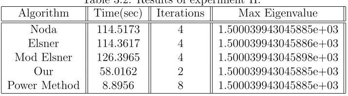
Experiment II: We use a positive random matrix which is generated by therand(n, n)
command in Matlab. In addition, we randomly replace some entries by 0 to create a new random nonnegative irreducible matrix. Table 3.2 shows the results when we apply all algorithms to the nonnegative random matrix size of n= 3000.
Table 3.2: Results of experiment II.
Algorithm Time(sec) Iterations Max Eigenvalue
Noda 114.5173 4 1.500039943045885e+03
Elsner 114.3617 4 1.500039943045886e+03 Mod Elsner 126.3965 4 1.500039943045898e+03
Our 58.0162 2 1.500039943045885e+03
Power Method 8.8956 8 1.500039943045885e+03
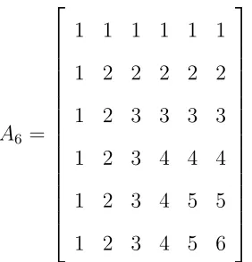
Experiment III: We use the matrix mentioned in the equation (3.14) of order n.
A6 =
1 1 1 1 1 1 1 2 2 2 2 2 1 2 3 3 3 3 1 2 3 4 4 4 1 2 3 4 5 5 1 2 3 4 5 6
.
Applying the formula from equation (3.15), we obtain that the exact value of ρ(A6) = 17.2068572.
Table 3.3: Results of experiment III when n = 6. Algorithm Time(sec) Iterations Max Eigenvalue
Noda 1.4299e-03 5 1.720685726740094e+01 Elsner 1.2319e-03 5 1.720685726740094e+01 Mod Elsner 5.4510e-03 6 1.720685726740095e+01
Our 1.8220e-03 3 1.720685726740094e+01
Power Method 1.1249e-03 9 1.720685726740095e+01
Next, we consider the case when n = 1000. The exact value of ρ(A1000) = 405690.203. Table 3.4 shows the results of all algorithms on A1000.
Table 3.4: Results of experiment III when n = 1000. Algorithm Time(sec) Iterations Max Eigenvalue
Noda 7.4830 5 4.056902039587474e+05
Elsner 7.5037 5 4.056902039587469e+05
Mod Elsner 8.1742 5 4.056902039587484e+05
Our 4.7143 3 4.056902039587469e+05
Power Method 1.4475 12 4.056902039587474e+05
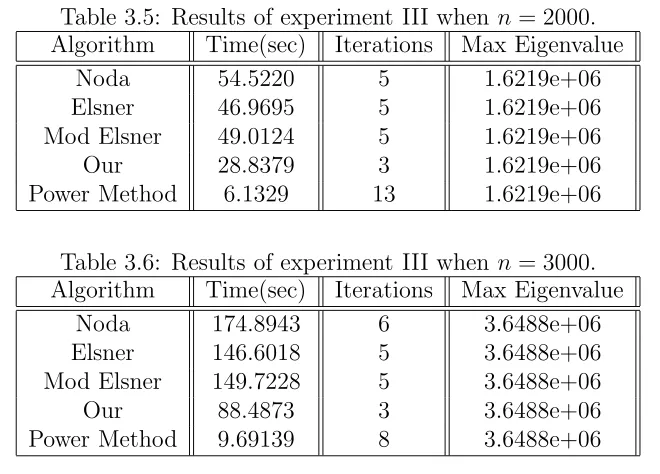
Table 3.5: Results of experiment III when n = 2000. Algorithm Time(sec) Iterations Max Eigenvalue
Noda 54.5220 5 1.6219e+06
Elsner 46.9695 5 1.6219e+06
Mod Elsner 49.0124 5 1.6219e+06
Our 28.8379 3 1.6219e+06
Power Method 6.1329 13 1.6219e+06
Table 3.6: Results of experiment III when n = 3000. Algorithm Time(sec) Iterations Max Eigenvalue
Noda 174.8943 6 3.6488e+06
Elsner 146.6018 5 3.6488e+06
Mod Elsner 149.7228 5 3.6488e+06
Our 88.4873 3 3.6488e+06
Power Method 9.69139 8 3.6488e+06
As the size of A increases, we see that our algorithm gives a better result than other algorithms.
Experiment IV: We consider the results for the computation of the Perron root of
a nonsymmetric tridiagonal Toplitz matrix in the equation (3.16) which can be represent by T(c, b, a, n) in the section 3.4. In this experiment, we use c = 2, b = 8, a = 5, and n= 800. Refer to the formula in equation (3.16), the Perron root of T(2,8,5,800) is ρ(T) = 1.432450667579053e+ 01, where the second largest eigenvalue is close to ρ(T).
Table 3.7: Results of experiment IV.
Algorithm Time(sec) Iterations Max Eigenvalue
Noda 99.131 119 1.432450667579053e+01
Elsner 104.5101 118 1.432450667579053e+01
Mod Elsner 104.2466 119 1.432450667579053e+01
Our 56.1995 66 1.432450667579053e+01
Power Method Does not converge
our algorithm are roughly about half of other algorithms required. In addition, the power method with Collatz’s formula does not converge.
In the next experiment, we run all algorithms on the perturbation matrix P in the equa-tion (3.18) which is a nonnegative and irreducible matrix. For each case in this experiment, we increase the sizenand decrease the value ofω.The authors of [17] also use these matrices to test the accuracy of their algorithm.
Experiment V: This is the perturbation matrix whose size n = 20 and ω = (0.5)20
(note that (0.5)20=9.5367e-007 ) defined as
P20(0.5)20 =
0 1 0 · · · 0 0 0 1 · · · 0
..
. ... ... ... ... 0 0 0 · · · 1 (0.5)20 0 0 · · · 0
20×20
. (3.20)
Using the formula given in the section 3.4, the Perron root of this matrix isρ= 0.5.
Table 3.8: Results of experiment V on P20(0.5)20.
Algorithm Time(sec) Iterations Max Eigenvalue
Noda 0.0236 14 0.5
Elsner 0.0172 13 0.5
Mod Elsner 0.0362 12 0.5
Our 0.0167 8 0.5
Power Method Does not converge
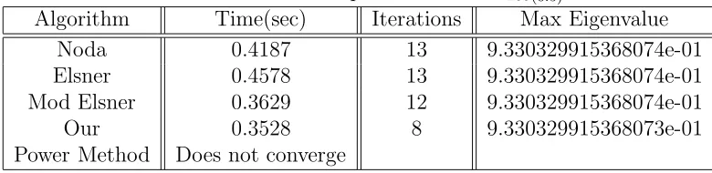
Table 3.9: Results of experiment V on P200(0.5)20.
Algorithm Time(sec) Iterations Max Eigenvalue
Noda 0.4187 13 9.330329915368074e-01
Elsner 0.4578 13 9.330329915368074e-01
Mod Elsner 0.3629 12 9.330329915368074e-01
Our 0.3528 8 9.330329915368073e-01
Power Method Does not converge
Interestingly, modified Elsner, Elsner, and Noda’s algorithm converge at the rate of quadratic [10]. Our algorithm overcomes all algorithms especially for a larger size of a nonnegative irreducible matrix. Below is the result when we test all algorithms on the perturbation matrix P500(0.5)20 with the size of n = 500 and ω = (0.5)20. The exact Perron root is ρ= 9.726549474122856e−01.
Table 3.10: Results of experiment V onP500(0.5)20.
Algorithm Time(sec) Iterations Max Eigenvalue
Noda 3.1728 13 9.726549474122854e-01
Elsner 3.0301 12 9.726549474122828e-01
Mod Elsner 3.5694 13 9.726549474123013e-01
Our 1.8613 7 9.726549474122880e-01
Power Method Does not converge
Next, we look at the case when n = 1000 and ω = 1e−16. The exact Perron root of P1000(1e−16) isρ= 9.638290236239705e−01.
Table 3.11: Results of experiment V on P1000(1e−16).
Algorithm Time(sec) Iterations Max Eigenvalue
Noda 31.3633 22 9.638290236239706e-01
Elsner 50.7471 35 9.638290236239713e-01
Mod Elsner 37.0038 24 9.638290236239708e-01
Our 19.4263 13 9.638290236239706e-01
Power Method Does not converge
formula produce the best result as we expected. However, our algorithm also produces good results compare to the power method and other algorithms; especially, when it computes the Perron root of large size matrices.
Chapter 4
Conclusions
In this dissertation we explored various methods for computing the Perron root of non-negative irreducible matrices. We produced a new algorithm. The proposed algorithm is based on the reciprocal of Collatz’s formula and the inverse iteration method. We have shown how our algorithm overcomes the three best known algorithms that use an inverse it-eration technique which converge to the Perron root at the rate of quadratic [10]. Moreover, our algorithm converges to the Perron root faster than other algorithms that employed the diagonal transformation technique and the Perron complementation idea.
We then took a closer look at the computational time of all algorithms including our algorithm on nearly reducible matrices. From all experiments, we found that our algorithm produced the best results. The experiments suggested our algorithm converges to the Perron root of nonnegative irreducible matrices at least quadratically.
Bibliography
[1] A. Ahac, J.J. Buoni, and D.D. Olesky. A stable lu-factorization of h-matrices. Linear algebra appl., 99:97–110., 1988.
[2] Pham Van At. Reduction of a positive matrix to a quasistochastic matrix by a simi-lar variation method. U.S.S.R. Computation Mathematics and Mathematical Physics., 11:255–262., 1971.
[3] Pham Van At. Reduction of an irreducible non-negativ matrix to quasistochastic form by the method similarity variation. U.S.S.R. Computation Mathematics and Mathematical Physics., 15:11–18., 1975.
[4] Robert G. Bartle and Donald R. Sherbert. Introduction to Real Analysis Third Edition. John Wiley and Sons, Inc, New York, 2000.
[5] Abraham Berman. Nonnegative Matrices in the Mathematical Sciences. Society for Industrial and Applied Mathematics, Philadelphia., 1994.
[6] A. Brauer. A method for the computation of the greatest root of a nonnegative matrix. SIAM J. Numer. Anal, 3:564–569., 1966.
[8] James W. Demmel. Applied Numerical Linear Algebra. Society for Industrial and Applied Mathematics, Philadelphia, 1997.
[9] Fujian Duan and Kecun Zhang. An algorithm of diagonal transformation for perron root of nnonnegative irreducible matrices. Applied Mathematics and Computation, 175:762– 772., 2006.
[10] Ludwig Elsner. Inverse iteration for calculating the spectral radius of a non-negative irreducible matrix. Linear Algebra Appl., 15:235–242., 1976.
[11] R.P. FEYNMAN. Statistical Mechanics. Benjamin,Reading, MA, 1972.
[12] Robert T. Gregory and David L. Karney. A Collection of Matrices for Testing Compu-tational Algorithms. Wiley-Interscience, New York, 1969.
[13] C.A. Hall and T.A. Porsching. Computing the maximal eigenvalue and eigenvector of a nonnegative irreducible matrix. SIAM J. Numer. Anal, 5:470–474., 1968.
[14] C.A. Hall and T.A. Porsching. Computing the maximal eigenvalue and eigenvector of a positive matrix. SIAM J. Numer. Anal, 5:269–274., 1968.
[15] T.E. Harris. The Theory of Branching Processes. Spring-Verlag, Berlin, 1963.
[16] R.A. Howard and J.E. Matheson. Risk sensitive markov dicision processes. Management Sci., 8:356–369, 1972.
[17] L.Elsner, I.Koltracht, M. Neumann, and D.Xiao. On accurate computations of the perron root. SIAM J. Matrix Anal. Appl., 14(2), April 1993.
[19] Linzhang Lu and Michael K. Ng. Localization of perron roots. Linear Algebra Appl., 392:103–117., 2004.
[20] M.S. Lynn and W.P. Timlake. Bounds for perron eigenvectors and subdominant eigen-values of positive matrices. Linear Algebra and Its Applications, 2:143–152., 1969.
[21] T.L. Markahm. An iterative procedure for computing the maximal root of a positive matrix. Math Comp., 22:869–871., 1968.
[22] C.D. Meyer. Uncoupling the perron eigenvector problem. Linear Algebra Appl., 114/115:69–94., 1989.
[23] C.D. Meyer. Matrix Analysis and Applied Linear Algebra. Society for Industrial and Applied Mathematics, Philadelphia, 2000.
[24] Michael Neumann. Inverses of perron complements of inverse m-matrices. Linear Alge-bra Appl., 313:163–171., 2000.
[25] Takashi Noda. Note on the computation of the maximal eigenvalue of a non-negative irreducible matrix. Numer. Math, 17:382–386, 1971.
[26] Tedja Santanoe Oepomo. A contribution to collatz’s eigenvalue inclusion theorem for nonnegative irreducible matrices. Electronic Journal of Linear Algebra, 10:31–45., 2003.
[27] A.M. Ostrowski. On the convergence of the rayleigh quotient iteration for the compu-tation of the characteristic roots and vectors. v. Archive for Rational Mechanics and analysis, 3:472–481, 1959.
[29] E. Seneta. Non-negative Matrices and Markov Chains. Springer-Verlag, New York, 1981.
[30] R.D. Skeel. Scaling for numerical stability in gaussian elimination. J. Assoc. Compt. Mach., 26, 1979.
[31] Slawomir Stanczak and Holger Boche. Information Theoretic Approach to the Perron Root of Nonnegative Irreducible Matrices. InProc. IEEE Information Theory Workshop (ITW 2004), pages 254–259, San Antonio, USA, October 2004.
[32] R.S. Varga. Matrix iterative analsis. Prentice-Hall Inc., Engwood Cliffs,N.J., 1962.
[33] J.H. Wilkinson. The Algebraic Eigenvalue Problem. Clarendon, Oxford, 1965.