An Approach to Determine Extent and Depth of Highway Flooding
Hubo Cai, PhD
URS Corporation – North Carolina 1600 Perimeter Park Drive, Suite 100Morrisville, NC 27560 Phone: (919) 461-1210 Email: [email protected]
William Rasdorf, P.E., PhD
Fellow, ASCEDepartment of Civil, Construction, and Environmental Engineering North Carolina State University
Campus Box 7908 Raleigh, NC 27695 Phone: (919)515-7637 Email: [email protected]
Chris Tilley
Application Analyst Programmer GIS Unit, NCDOT 1587 Mail Service Center Raleigh, N.C. 27699-1587 Phone: (919) 212-6040 Email: [email protected]
Key Words
Flood Hydrology Flood Peaks
Floods Disaster Response Transportation Corridors Transportation Networks Highway Management
An Approach to Determine Extent and Depth of Highway Flooding
ABSTRACT
INTRODUCTION
MODELING Water Bodies Flooding
LITERATURE REVIEW AND MOTIVATION
METHODOLOGY
Flood Extent and Depth Prediction Flooded Road Segment Identification Data Sources
Algorithms for Flood Extent and Flood Water Level Enforcement of Constraints
Algorithm for Identifying Flooded Road Segments and Water Depth
CASE STUDY Study Area Test Results
APPLICATIONS OF THE RESEARCH
LIMITATIONS AND CONCLUSIONS
REFERENCES
Words: 7430 Figures: 16
ABSTRACT
Flooding and flash flooding pose serious infrastructure hazards to human populations in many parts of the world. Under a flooding scenario, it is critical to identify road segments that are flooded so that rescue and response routes can be determined and rescue personnel and supplies can be distributed promptly and in a timely manner. Presently there is no such information system that would accurately predict flooded road segments and their depth given a specific flood level and provide this information for rescue activities.
INTRODUCTION
Flooding and flash flooding pose serious infrastructure hazards to human populations and the built environment in many parts of the world. According to FEMA, floods are the second most common and widespread of all natural disasters (Noman et al. 2001). North Carolina faces extreme hazards and consequences from flooding, particularly those caused by hurricanes. Since 1989, there have been 14 federally declared disasters in North Carolina. Damage from Hurricane Floyd alone has reached $3.5 billion and destroyed 4,117 uninsured and under-insured homes (NCCTSFMP 2000).
The nation’s transportation infrastructure plays a critical role in hurricane events by providing rescue routes under a flooding scenario. In order to efficiently utilize the existing transportation infrastructure system in rescue, we must identify road segments that are flooded and road segments that are not flooded so that rescue and response routes can be determined and rescue personnel and supplies can be distributed promptly and in a timely manner (Cai 2003). Furthermore, we need to determine flooding depth on the road surfaced itself. However, currently there is no information system that can accurately identify flooded road segments during an emergency event and provide this information for rescue activities. It is not unusual for a rescue team to use a road before realizing that part of that road is flooded and becomes an impassable barrier. This causes expensive delays in response activities that cost not only property damages, but also lives. Therefore, it is extremely important to establish an accurate prediction system to support rescue activities under a flooding scenario.
Most states in the US collect and maintain flood maps. It is quite natural to turn to these flood maps for help in determining rescue and response routes under a flooding scenario because no other resource often exists. But there are problems with using flood maps for the purpose identified here. First, flood maps categorize areas into 100-year flood zones, 50-year flood zones, 20-year flood zones, etc. They predict the flood risk for areas rather than anything else and have no true connection to the transportation network. Therefore, it is far from ideal to use flood maps to identify road segments under flood conditions. Second, when a flood occurs, road segments in the flooded area might not be flooded at all or they might just be partially flooded and in reality, could be used as rescue routes.
This paper reports on a study to develop a prediction prototype to determine flooded road segments under a flooding scenario. By doing so, the flooded road segments could be identified in a timely manner to help determine rescue routes. The paper presents the development of models and algorithms for assessing highway flood scenarios and the results from the prototype. We did not conduct a series of tests to fully validate the model at this time.
MODELING
In a general flooding scenario water levels rise and result in neighboring areas and some road segments in these areas being flooded. This section describes spatial modeling of water bodies and provides brief descriptions of various flooding scenarios.
Water Bodies
Flooding
There are two aspects of interest to us regarding flooding: first, the water body floods (flooded water level is higher than normal) causing water flows to the surrounding areas; and second, the flowing water interacts with roads, covering road segments. This section deals with the first of these; the next section deals with the second. The extent to which water flows to surrounding areas depends on the water surface level, the surface or elevation changes of surrounding areas, and slopes. Determining which road segments are flooded depends on the elevations of the road and the flood level.
Figure 1 shows a cross-sectional view of how a water body can flood and how water reaches surrounding areas. The normal water level is the water surface level before a flood occurs. The flooded water level is the water surface level at the time the flood occurs. The difference between the flooded water level and the normal water level is defined as the flood level. In Figure 1, the water level increases from the normal water level to the flooded water level. It is obvious that there are surrounding areas that were not under water before flooding but are under water after flooding (areas having elevations higher than the normal water level but lower than the flooded water level). The dashed line represents another flooded level, in which area A is not flooded even though its elevation is lower than the flooded water level because feature B has become a natural barrier to water flow into area A.
Figure 1 Cross-sectional View of Flooding
Flood Impact on Roads
Of particular interest in this paper is Figure 2 which provides a profile of a road segment with several portions of the road under water. As illustrated in Figure 2, part of the road segment may not be flooded even though it is in the flooded area because a road is a three-dimensional object with elevations changing along its length and parts of it may be above flood level. The challenge is to find those portions that are flooded and to determine their depth so that appropriate response actions can be taken.
Figure 2 Illustration of Flooded and Not Flooded Road Segments in the Flooded Area
As shown in both Figures 1 and 2, in order to predict and identify flooded road segments, at least two models need to be developed. The first one predicts the extent to which water flows when flooding, based on the elevations of surrounding areas and the surface water elevation. The second identifies flooded road segments for roads running through those flooded areas. We use a simplified model for the first. Our primary contribution lies in the second. That is, the determination of accurate 3D road centerline coordinates is critical to identifying flooded portions of roads. Our primary purpose is to present how these are obtained. The centerline coordinates of flooded portions of roads can then be used for many applications.
Road Profile
Segments Flooded Segments Not Flooded Flooded Water Level
Normal Water Level Flooded Water Level
Area A Feature B
LITERATURE REVIEW AND MOTIVATION
Flood extent prediction, or floodplain delineation is the process of determining inundation extent and depth by comparing river water levels (the elevation of the water surface) with ground surface elevations (Noman et al. 2001). The traditional method of floodplain delineation is to use a topographic map (Noman et al. 2001). This method consists of marking the water levels from the observations of river stages on the topographic map, extending the water level until impeded by the higher elevation contour, tracing the contour lines to delineate the floodplain, and manually producing a flood extent map.
In an automated approach, the procedure is the same but the topographic map is replaced with a digital terrain model (DTM) and results from a hydraulic model either replace or supplement the observations of river stages to obtain water levels (Noman et al. 2001). Based on the water level points, a water level surface is created and compared to the DTM to produce an automated flood depth and extent map. Much research has focused on automatically delineating and mapping floodplains using DTM and further applying GIS technology (Noman et al. 2001, Noman et al. 2003, Tate et al. 2002, Radaideh et al. 2004).
With the use of Light Detection and Ranging (LIDAR) to acquire highly accurate elevation datasets, the accuracy of the resulting floodplain maps has improved (Stonestreet and Lee 2000, Wang and Zheng 2005). But it has been found that many rivers have existing levees formed by structures such as roads, which are usually not well represented in a DTM but which do affect water levels during a flood event (Shapiro and Nelson 2004). Recognizing culvert structures might be improved by using high resolution DTMs such as those created from LIDAR. However errors will not entirely be eliminated unless roads are specifically taken into consideration.
A fairly recent development in the field of floodplain delineation has been the coupling of hydraulic modeling and GISs (Tate et al. 2001, Demissie et al. 2001, Shapiro and Nelson 2004). With GISs, the stream cross-section parameters are extracted from a digital terrain model and imported into a hydraulic model to be processed to produce results regarding the floodplains (Tate et al. 2001). Computing models and tools such as the Engineering Center River Analysis System (HEC-RAS) and HEC-GeoRAS from the U. S. Army Corps of Engineers are available to integrate GISs with hydraulic modeling in this manner (Bennett et al. 2004, HEC-GeoRAS 2005). These technologies, models, and tools have been applied in many floodplain assessment studies (Lauer and Parker 2004, Schalk et al. 2001, WW&ERC 2001).
Most existing research efforts focus on floodplain delineation only. On the other hand, most research efforts in transportation infrastructure systems focus on the performances and sustainability of roads and bridges with varying designs and materials. The critical role of transportation infrastructure systems in flood rescue has been recognized for a long time. However, there is a lack of literature regarding how to identify either the extent of flooded road segments and how to determine their flood depth under a flood event so that decisions regarding evacuation and rescue routing could be made to be more efficient, more timely, and more accurately. This motivated the authors to develop a prototype of such a prediction system. This requires an integration of a highly accurate roadway network model with floodplains under a flood event so that flooded road segments can be identified.
METHODOLOGY
This section describes models and algorithms developed to predict flood extent using flood depth information and to subsequently identify flooded road segments.
Flood Extent and Depth Prediction
It is recognized that water level varies throughout a water body as in the case of a river. It is infeasible to assume a uniform normal water level and a uniform flooded water level in a relatively large geographic basin. However the flooded water level always equals the sum of the normal water level and the flood level as described earlier. This relationship between the flooded water level and the normal water level provides an alternative to determine the flooded water level other than obtaining flooded water levels at different locations via direct measurements or using the results from a hydraulic model. This alternative approach assumes that the flooded water surface is equivalent to the normal water level before flooding plus the flood level. The normal water level before flooding at a given point is assumed to be equivalent to the elevation of that point from a high-resolution DTM such as a LIDAR DEM (NCFMP 2003). It is reasonable to assume a uniform flood level in a relatively small geographic basin. The normal water level, which varies over a particular geographic basin, together with the assumed uniform flood level, provide inputs to a simplified flood extent prediction model that is described in detail in the following paragraphs.
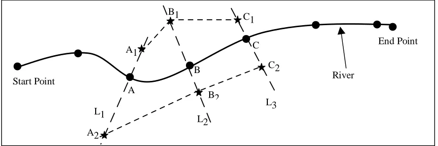
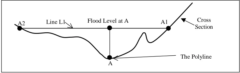
Figure 3 illustrates, in a simplified way, how the prediction model predicts the flood extent and depth information with a given flood level (the increase of water surface level from its normal level when flooding). In Figure 3, the river is represented as a polyline. Figure 4 shows the area in cross section. A few points that are uniformly distributed along the polyline (with the same interval) starting from the start point of that polyline are obtained. In addition, the start and end points of the polyline are obtained.
At each of the identified polyline points (A, B, C), a line normal to the river polyline is constructed. For example, at point A, a normal line L1 is constructed. Along this line L1, two points (A1 and A2) are identified (see Figure 3). These two points are on two different sides of the river polyline and have elevations equivalent to the elevation at point A plus the given flood level. For example, if point A has an elevation of 105 ft and the given flood level is 2 ft, points A1 and A2 are assumed to have the same elevation of 107 ft. A set of straight lines will be produced by performing this process with every point and consequently a set of neighboring polygons are constructed by closing neighboring lines. For example, two polygons (polygon A1A2B2B1 and polygon B1B2C2C1) can be constructed by closing lines A1A2 with B1B2 and by closing lines B1B2 with C1C2. Each of these polygons will have a water level, which takes the average of elevations at points A and B (and B and C) plus the given flood level.
Figure 3 Conceptual Model for Predicting Flood Extent
This simplified flooding model represented in this paper enables us to determine both the flooded water level and the extent to which the flooded water is dispersed to surrounding areas. Other flooding models such as the HEC-GeoRAS mentioned in the literature review section could also be used to provide flood level information/inputs and consequently, determine the flooded water level and the flood extent. For example, part of the outputs from running HEC-GeoRAS is 1) a water surface dataset in the format of a triangulated irregular network (TIN) or a raster/grid and 2)a depth dataset in the format of a raster/grid. These datasets can be processed and utilized to determine the flooded water level and the flood extent. The main point of this paper is not to develop new models for flooding, but to evaluate the impacts on roads of flooding with different flood levels.
There are two constraints to be recognized. The first constraint is based on the fact that, for a water body, the elevation of the place where the water body is located is lower than the elevations of the surrounding areas in all
Start Point River
End Point
A1 C
B
A
L1
L2
L3
A2
B1
B2
C1
directions but the direction of flow. The second constraint comes from a fundamental characteristic of a water body, water always flows from higher levels to lower levels. That is, along the water flow direction water surface levels are always decreasing.
Figure 4 Sample Cross Sectional Illustration of Normal Line Construction
Flooded Road Segment Identification
As stated earlier, if a road segment is within a flooded area, it does not mean that the whole road segment is under water. For a road segment in the flooded area, it is very possible that only parts of that road segment is flooded as was illustrated in Figure 2. The main goal of our flooded road segment identification model is to identify those parts and differentiate them from the rest of the road segment.
Information Sources
Three information sets are required: water body data, LIDAR DEMs, and 3-D Road information. The LIDAR DEMs are used in conjunction with water body data to determine flood extent and depth as described above and as shown in Figure 3. The road information is then used in conjunction with these to establish the flood extent and depth on the road itself as shown in Figure 2.
The water body data are in the format of a line shapefile. This data was provided by the GIS Unit of the North Carolina Department of Transportation (NCDOT). The LIDAR DEMs were provided by the North Carolina Floodplain Mapping Program (North Carolina Flood Mapping Program 2003). This program is undertaking the LIDAR survey in NC to obtain elevation data with a high accuracy and consequently, to produce flood maps statewide. The LIDAR DEMs have a resolution of 20 ft with a vertical root mean square of error (RMSE) of 25 cm on bare, hard, flat surfaces with 1 meter being more common on grassy or other sloped or softer surfaces. LIDAR data in other formats (hydro DEMs with a resolution of 50 ft and bare earth mass points with X/Y/Z-coordinates in ASCII files) is also available. LIDAR provides a highly accurate elevation dataset and, as a result, it is being used widely in floodplain mapping (North Carolina Flood Mapping Program 2003). There is also a pilot study in North Carolina that uses LIDAR to locate first and second-order streams (Garcia 2004). These studies seem to support the use of LIDAR in floodplain-related investigations and applications.
The road information consists of a 3-dimensional road centerline data model obtained from a previous study by the authors. Each road segment is associated with a set of 3-D points (with X/Y/Z-coordinates) along the road segment. For these 3-D points, their X/Y-coordinates were obtained from NCDOT LRS road data and their Z-coordinates were obtained from 3-D LIDAR points (Cai 2003, Rasdorf 2003, Rasdorf 2004). In order to assure positional accuracy, the planimetric position of the road centerlines was obtained by digitizing orthorectified aerial photos. LIDAR points were used to introduce the third dimension – elevation (Cai 2003, Rasdorf 2003, Rasdorf 2004). The average density of these 3-D points along road segments is approximately 15 ft. For data sharing purposes, the 3-D road centerline data are in the format of framework transportation segments (FTSeg) based on recommendations from the Federal Geographic Data Committee (FGDC) and the Federal Highway Administration (FHwA) (FGDC 1994, FGDC 1999, FHwA 1998).
To summarize, the water body data are two-dimensional linear data. The road data are three-dimensional data, which are represented as straight line segments connecting 3-D points along road segments. The LIDAR DEMs are
Flood Level at A Line L1
The Polyline A
Cross Section A1
the elevation data being used to describe the surface. The coordinate system being used is the State Plane Coordinate System with measurements given in feet. The horizontal datum is NAD83. The vertical datum is North American Vertical Datum of 1988 (NAVD88) with measurements given in feet. All datasets are reprojected into the same coordinate system.
Algorithms for Flood Extent and Flood Water Level
This section describes the algorithms developed to predict the flood extent and depth using water body data, elevation data, and a given flood level. Figures 5 and 6 describe the algorithms developed to extract points from water lines, construct normal lines, identifying target points, and construct polygons to simulate flood extents with depth information.
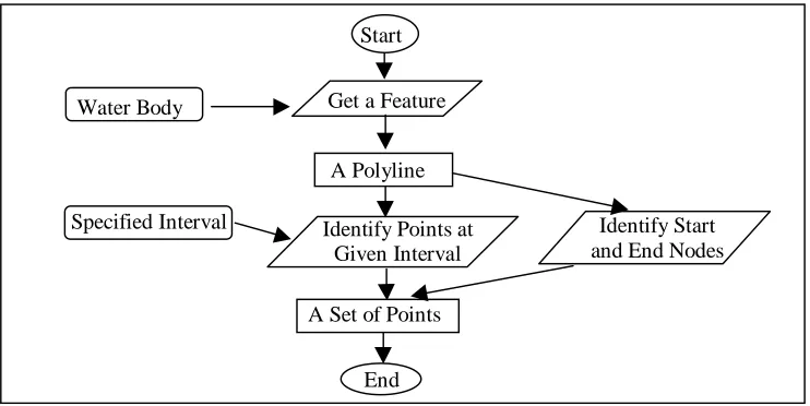
Figure 5 illustrates the algorithm used to obtain points along a polyline. In Figure 5, a polyline feature is obtained from the water body data (a line shapefile). By identifying the start and end nodes of this polyline and identifying points along the polyline, which are uniformly distributed (uniform interval) at the specified interval from the start point, a set of points are obtained for the analysis. The uniform interval is at the size of the resolution of the LIDAR DEM, i.e. 20 feet. As a general rule for working with raster data, the smaller the interval, the more accurate the results will be. However, if the interval reaches cell resolution, the accuracy will not be improved by further reducing the interval (Cai 2003).
The reason of using a uniform interval to obtain points along a polyline instead of using the vertices of this polyline is that these vertices are not uniformly distributed. In other words, the distance between two neighboring vertices along the line varies and using these vertices will affect the accuracy of the results. Repeating this procedure for all features in the water body dataset results in sets of points (points A, B, and C in Figure 3, for example). Each set is associated with a polyline feature describing the water body.
Figure 5 Obtaining Points along A Polyline
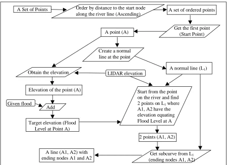
Figure 6 describes the procedure of constructing normal lines to the water body polyline at those points identified in Figure 5. First, the set of points describing a polyline (obtained from the procedure just described) is placed in ascending order by distance from the start node. For each of these points, a line normal to the polyline is constructed based on the curvature of the polyline by using the QueryNormal method available from the ArcObjects GIS software. The elevation at the point is determined based on the LIDAR DEMs (point A in Figure 3, for example). The target elevation (the flooded water surface level) at this point (flood level A in Figure 3A for example) is determined by adding the given flood level to the elevation of the point.
Two corresponding points on the normal line, which have the same elevations as the target elevation, are then identified (points A1 and A2 in Figure 3, for example). The procedure for doing so is discussed in the next section. After A1 and A2 are identified, a straight line connecting A1 and A2 can be constructed and later on, this line will
Start
Water Body
End Get a Feature
A Polyline
Identify Start and End Nodes
A Set of Points Identify Points at
be used together with another such line being constructed at the neighboring points of point A to construct polygons that represent the flood extent.
Figure 6 The Procedure of Predicting Flood Extent
The critical part of this procedure is how the two points A1 and A2 are identified based on the elevation data. Figure 7 illustrates this identification procedure in detail. In Figure 7, line N1 is the normal line constructed at point A. Point A1 is the point that has the target elevation and is the point that needs to be identified. The procedure is described as follows (LIDAR DEMs are used as the elevation grid).
Figure 7 Identifying Points with Target Elevation A Set of Points
Create a normal line at the point
A line (A1, A2) with ending nodes A1 and A2
A point (A) Get the first point(Start Point) A set of ordered points Order by distance to the start node
along the river line (Ascending)
Obtain the elevation A normal line (L1)
Get subcurve from L1
(ending nodes A1, A2) 2 points (A1, A2)
Start from the point on the river and find 2 points on L1 where
A1, A2 have the elevation equating Flood Level at A LIDAR elevation
Target elevation (Flood Level at Point A)
Add
Elevation of the point (A)
Given flood
A A1
T1 T2 T3
L1
Polyline Elevation
Grid
1) The elevation of the cell in which point A is located is obtained.
2) Elevation at point A is added with given flood level to obtain the target elevation.
3) Starting from point A along the normal line, point T1 is identified by its distance from point A. The distance between A and T1 equals the resolution of the elevation grid file (the height or width of a cell).
4) The elevation of the cell containing point T1 is obtained and compared to the target elevation. If this elevation is lower than the target elevation, another point T2 along the normal line is obtained. The distance between T2 and T1 again equals the resolution of the elevation grid file. The elevation of T2 is compared to the target elevation. This step is repeated until the first point having an elevation higher than the target elevation is obtained.
5) Assuming that the first point having an elevation higher than the target elevation is T3, this indicates that point T2 has an elevation lower than the target elevation. Taking a linear interpolation approach, we identify a point A1 between T3 and T2 on the normal line that has an elevation equal to the target elevation. This point A1 is the point sought.
6) Repeat steps 3) to 5) to identify point A2 on the other side.
Clearly, the accuracy of both the position and elevation of points A1 and A2 are dependent on the accuracy of the LIDAR DEM. Thus, the reader is cautioned that a quality dataset at a reasonable resolution is required to obtain the best results. The point is that if such due diligence is shown a high quality result will be obtained.
Enforcement of Constraints
The algorithm illustrated in Figure 6 utilizes the results from the execution of the algorithm illustrated in Figure 5, i.e. sets of points along the polyline. The two constraints stated earlier are enforced by examining the elevations of the resulting points from the algorithm illustrated in Figure 5. These resulting points must be examined before the execution of the algorithm illustrated in Figure 6 to assure that the constraints are enforced.
The first constraint states that the elevation of a point on the polyline representing the water body must be lower than the surrounding areas except those neighboring points in the flow direction. This constraint is enforced by comparing the elevation value of the cell (from the grid representing the surface elevations) containing that particular point with the elevations of the eight neighboring cells. If this constraint is not satisfied, the elevation for this particular point is adjusted by taking the elevation of the immediate neighboring downstream point.
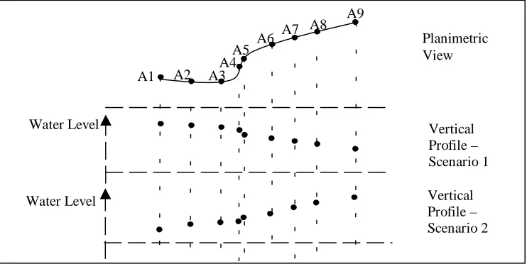
The second constraint states that water flows in the direction of higher to lower elevations. Figure 8 illustrates this situation. Theoretically, if water flows from point A1 to point A9, then the water levels of points A1 to A9 should appear as shown in vertical profile scenario 1. If water flows from point A9 to point A1, then the water levels of points A1 to A9 should appear as shown in vertical profile scenario 2. While this is intuitive to us it requires search and test procedures for software.
Figure 8 Water Flow Direction Illustration
A1 A2 A3
A4A5
A6 A7 A8 A9
Water Level
Water Level
Planimetric View
Vertical Profile – Scenario 1
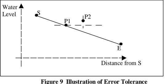
Examining the points along the polyline after enforcing the first constraint reveals that it is not always the case that these points would follow the water flow rule due to errors in the waterline position and the elevation dataset. In order to ensure that water is always flowing downward, the elevations of the points along the polyline are adjusted. This adjustment could be implemented using an error tolerance constant (in units of ft/ft) such as illustrated in Figure 9. These two constants vary depending on the area where the developed models are being applied.
Figure 9 Illustration of Error Tolerance
In Figure 9, a straight line is used to represent the vertical profile of the water surface levels (S to E). The horizontal axis represents the planimetric distance from the start point of the polyline under consideration. The vertical axis represents the water surface level.
Assume that water flows from the start point S to the end point E. LIDAR points P1 and P2 are two neighboring points. Ideally, these points are on the straight line representing the vertical water profile and point P2 is lower than P1. However, Figure 9 illustrates that point P2 is higher than point P1. In other words, an error occurs. This error is mainly caused by the positional inaccuracy of water data. The maximum extent of this error, which is acceptable, is defined as the error tolerance. Thus, in the scenario illustrated in Figure 9, if the error exceeds the given error tolerance, an adjustment is required, which assigns the water level of point P1 to point P2. This adjustment is similar to "burning streams into DEM," i.e., adjusting DEM by taking streams into consideration. The difference is that “burning streams into DEM” modifies the DEM for later analysis while this adjustment works on the results without modifying the DEM.
Using this algorithm, the flood extent is determined. The flood extent consists of numerous polygons. Each of these polygons has a flood level elevation value. This set of data will be used later to identify road segments that are under water.
Algorithm for Identifying Flooded Road Segments and Water Depth
After the flood extent and depth information is obtained by implementing the flood extent prediction model as described above, a set of small polygons are created. These polygons represent the areas that are under water. Each polygon is assigned a value representing the flood water level. This information is used together with the 3-D road centerline data to identify road segments that are flooded. In our study, a 3-D road centerline is represented with a set of 3-D points (black dots in Figure 10). Each of these 3-D points has X,Y, and Z-coordinates.
S
E
P1 P2
Water Level
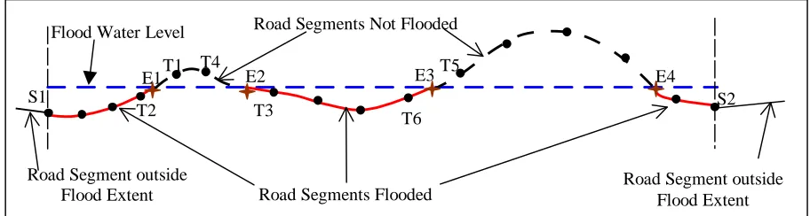
Figure 10 Road and Flood Profile Schematic
Figure 10 illustrates the scenario of determining flooded road segments for the road segment S1S2 that is in the flood extent. The black points represent all 3-D points on the road segment. Except for the start and end points, all these points come directly from the 3-D road data. For the start and end points, their elevations are obtained by linear interpolation. For example, for the start point, its elevation is linearly interpolated from its two neighboring 3-D points.
As illustrated in Figure 10, road segment S1S2 is within the flood extent. However, this road segment is not completely flooded. The goal is to identify the break points E1, E2, E3, and E4 in Figure 10 with elevations equivalent to the flood water level. These break points do not directly coincide with the existing points along the road centerline. They are obtained by identifying point pairs (such as the point pair T1 and T2) that consist of their two neighboring points, of which, one point has its elevation lower than the flood water level while the other has its elevation higher than the flood water level. The position of the break point is obtained by linear interpolation. By doing so, all break points are identified and consequently, portions of this road segment under water (S1E1, E2E3, and E4S2) are determined.
It is clear that there are two tasks for determining road segments under water. The first task is to determine road segments that are within the flood extent. The second task is to identify the under water portions of a given road segment that is within the flood extent. Finally, at any point along a flooded road segment the water depth can be determined.
Figures 11 and 12 illustrate, respectively, the algorithm for determining road segments within the flood extent and the algorithm for determining under water portions of a given road segment that is determined to be within the flood extent. The former is simply an overlay operation, i.e. the road centerline data are overlaid with the polygon data representing the flood extent. When this is done, road segments that are located within the flood extent are identified.
Figure 11 Flooded Road Segment Identification Algorithm, Part I
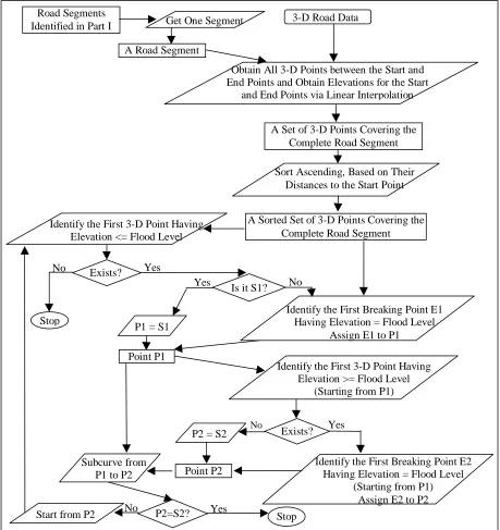
For each of the road segments identified, the algorithm illustrated in Figure 12 is carried out to determine under water portions of that road segment. This algorithm works in such a way that first, a set of 3-D points between the start and end points of the segment are obtained from the 3-D road data. In addition, the start and end points of the identified road segment are obtained and their elevations linearly interpolated from the 3-D road data. With a set of
Get a Feature
A Flood Extent Polygon with
Flood Level A Road Segment
Overlay Road Segments in the Flood Extent Polygon
Flood Extent Data Get a Feature 3-D Road Data
Flood Water Level Road Segments Not Flooded
Road Segments Flooded Road Segment outside
Flood Extent Road Segment outsideFlood Extent
S1 S2
T1
T2
E2
T3
T4 T5
T6
points covering the complete road segment, all break points with their elevations equivalent to the flood water level are identified, and consequently, all portions of this road segment that are under flood are identified. Two points variables (P1 and P2) are used to store the corresponding starting and ending points of the under water portions of the given road segment.
Figure 12 Flooded Road Segment Identification Algorithm, Part II
CASE STUDY
This section describes the results of executing the flood extent prediction model, the model for identifying portions of road segments under water, and their corresponding algorithms.
Study Area
The study area for applying the models and algorithms was chosen to be part of the Wilson County in North Carolina. There are a number of reasons for choosing the study area (illustrated in Figure 13). First, there is
high-Road Segments
Identified in Part I Get One Segment
A Road Segment
3-D Road Data
Obtain All 3-D Points between the Start and End Points and Obtain Elevations for the Start
and End Points via Linear Interpolation
A Set of 3-D Points Covering the Complete Road Segment
Sort Ascending, Based on Their Distances to the Start Point
A Sorted Set of 3-D Points Covering the Complete Road Segment Identify the First 3-D Point Having
Elevation <= Flood Level
Exists? Yes No
Identify the First Breaking Point E1 Having Elevation = Flood Level
Assign E1 to P1 Stop
Point P1
Identify the First 3-D Point Having Elevation >= Flood Level
(Starting from P1)
Exists? Yes
No
Identify the First Breaking Point E2 Having Elevation = Flood Level
(Starting from P1) Assign E2 to P2 P2 = S2
Point P2 Subcurve from
P1 to P2
P2=S2? Yes No
Stop Start from P2
Is it S1?
Yes No
quality water body data in this area. Second, LIDAR data are also available in this area. Third, 3-D road data is available in this area. Fourth, there are roads that are close to the water body and therefore, will produce meaningful results. While only portions of roads and water bodies in Wilson County are included in the application scope, the LIDAR elevation data are available for the entire county.
Figure 13 Study Scope Within Wilson County
Results
The flood extent prediction model and its associated algorithm were tested with the water body data in the study scope. The initial interval of the points along the river is 20 ft, which is the same as the cell size of the elevation data (LIDAR 20-ft DEMs). The selected flood level was 2 ft. Figure 14 shows the results of flood extent prediction, using algorithms described in the subsection of Enforcement of Constraints to deal with the error tolerance and the maximum drop issues. Both algorithms use an error tolerance of 1ft/10ft and a maximum drop of 1ft/50ft. These two parameters are based on values that are typical in Eastern NC and were obtained from professional engineers from the Hydraulics Unit of the NCDOT.
After the flood extent is determined using a given flood level and interval, the flooded road segment identification model and its associated algorithm can be applied to identify flooded road segments. In applying this model and its algorithm, the 3-D road data mentioned earlier play a critical role.
Figure 15 shows the results of applying this model when using the results of the flood extent model with a flood level of 2 ft, using algorithm 1. Figure 15 shows the results of applying this flooded road segment identification model using the results of the flood extent model with a flood level of 2 ft, using algorithm 2. Comparing these two reveals that even though two different algorithms are used to determine flood extent, the resulting identified under water portions of road segments are almost the same. Figure 16 provides a detailed view of the identified flooded road segments. It is obvious that for a road segment within the flood extent it does not mean that this road segment is completely flooded.
APPLICATIONS OF THE RESEARCH
The results of this research include the predicted flood extent on the terrain surface, the predicted flood extent on roads, the flood/water depth on the terrain surface, and the flood/water depth on the road surface.
roads requires that a maximum water depth on roads not be exceeded. Presented as results of this research, the flood extent and depth information on the terrain surface and roads predicted in this research enables the applications mentioned above to be supported.
In addition, the results of this research can be applied in other applications. For example, this research can help identify critical areas of damage both during and after a flooding scenario. It can predict the number of businesses that were flooded for assessment and timely repair. It helps to identify flooded animal habitats and wetlands that are critical to environmental and ecological health. It can also help establish locations for relief and rescue operations and find critical infrastructure systems (power stations, for example) that were or were not flooded and can still be used in the disaster recovery activities. This research can also identify infrastructures other than roads, which could be damaged. For example, given elevations of rails the impacts on the railroad industry from flooding can be determined.
Clearly there are numerous applications that can benefit from the result of this study. A comprehensive list of such applications and how this research can benefit those are beyond the scope of this paper and therefore, only a few applications were listed and briefly described above, as examples.
Figure 15 Flooded Road Segments
Figure 16 Detailed View of the Flooded Road Segments Legend
Interstate Highway Flooded Road Segment
Flood Extent
Legend
LIMITATIONS AND CONCLUSIONS
It is recognized that the two models (the model for flood extent prediction and the model for determining under water portions of road segments) developed in this study have limitations. The flood extent prediction model assumes a uniform flood level (a uniform water surface level increase) for all water bodies in the study scope. We recognize that, in reality, this is not the case. However, it was reasonable to assume a uniform flood level in a relatively small area. For a relatively large study area, it would be more reasonable to divide it into smaller areas and assume a uniform, but different flood level for each of them. Other models could also be used.
There is also in the case of local peaks, i.e. the flood water can go around and surround the peak. Our model for flood extent prediction will miss this other side. This limitation can be mitigated by obtaining more densely distributed points along the streamlines, but will not be avoided completely. This limitation indicates an opportunity of enhancing the flood extent prediction model in this study. However, doing so was not immediately necessary since the focus of this work was on combining a previously unavailable 3D road centerline model with any one of many flood models. Finally, in enforcing the two constraints, an error tolerance and a maximum drop were used. Their values will differ if areas other than the Wilson County Study Area are investigated.
One additional limitation of this model is the fact that, in using LIDAR surface data, the model does not "see," and therefore does not account for, culverts. These support the creation of water flow paths that otherwise would not exist. This directly affects flood extent but affects overall flood level to a lesser degree. We would recommend that these be incorporated into future studies.
We conclude that, based on the study results, the models presented here provide a simplified, yet practical and flexible approach to determine flood extent and depth and for identifying road portions under water. We hope that further testing will bear this out. Users are provided with the flexibility of using different flood levels in different areas under different flooding scenarios. The error tolerance and maximum drop could be customized to cope with different geographic areas and with varying natures of different water bodies. The integration of 3-D road centerline data with flood extent and depth information provides a practical way in determining flooded road segments and consequently, useful information could be obtained to determine escape and rescue routes. Compared to varying planimetric road centerlines data, the use of 3-D road centerlines provide more detailed information regarding the flooded road segments. It is believed that with accurate flood extent and depth information, the use of 3-D road centerline data would significantly benefit emergency response and management activities such as those in the scenarios of hurricanes and floods.
The significance of this work is that it uses LIDAR data to obtain the most accurate model of road centerlines possible, it uses LIDAR data to determine a model of flood extent, and it combines the two to provide flood extent on roads as well as flood water depth. It does so more accurately than ever before because such precise data on road location has not been previously been available. Previous work was based only on contours or DEMs created from sources other than LIDAR. These are much less accurate than the LIDAR DEMs used in this study. No previous study had a highly accurate separate roadway model available to it.
ACKNOWLEDGEMENT
The authors are grateful to the National Science Foundation for funding portions of this work through NSF Grant No. 9978592. The authors are also grateful to the GIS Unit of NCDOT for co-funding this work and for providing data, equipment, and software packages for completing the work.
REFERENCES
Cai, H. (2003). Accuracy Evaluation of a 3-D Spatial Modeling Approach to Model Linear Objects and Predict their Lengths, PhD Dissertation, Department of Civil Engineering, North Carolina State University, Raleigh, NC, November.
Demissie, M., Lian, Y., and Bhowmik, N. G. (2001). “Application of Hydraulic Models for the Analysis of the Interaction of the Illinois River and its Floodplain,” Bridging the Gap: Meeting the World’s Water and Environmental Resources Challenges, State of the Practice—Proceedings of the World Water and Environmental Resources Congress, May 20-24, 2001, The Rosen Plaza Hotel, Orlando, Florida, American Society of Civil Engineers, Section 1, Chapter 23.
Federal Geographic Data Committee (FGDC). (1999). National Spatial Data Infrastructure Framework Transportation Identification Standard – Working Draft, FGDC Ground Transportation Subcommittee, May.
Federal Geographic Data Committee (FGDC). (1994). Subcommittee Reports: FGDC Ground Transportation Subcommittee Positions and Recommendations on Linear Referencing Systems, FGDC Ground Transportation Subcommittee.
Federal Highway Administration. (1998). Linear Referencing Practitioners Handbook, prepared for FHWA contract #DTFH61-95-C-00169, Task Order 5 by GIS/Trans, Ltd.
Garcia, V. (2004). Automated Techniques to Map Headwaters Stream Networks in the Piedmont Ecoregion of North Carolina, Master Thesis, Forestry Department, North Carolina State University, Raleigh, NC, May.
HEC-GeoRAS. (2005). “HEC-GeoRAS,” http://www.hec.usace.army.mil/software/hec-ras/hecras-hec_georas.html, U. S. Army Corps of Engineers, Accessed March 01.
Lauer, J. W. and Parker, G. (2004). “Modeling Channel-Floodplain Co - Evolution in Sand-Bed Streams,” Critical Transitions In Water And Environmental Resources Management, Proceedings Of The 2004 World Water and Environmental Resources Congress, June 27 - July 1, 2004, Salt Lake City, UT, American Society of Civil Engineers, Pages 1-10.
NCCTSMP. (2001). “Issue 5: Quality Control of LIDAR Elevation Data in North Carolina, http://www.ncgs.state.nc.us/flood/ip05_nc_lidar_qc.dbf, Accessed October.
North Carolina Flood Mapping Program (NCFMP). (2003). “North Carolina Flood Mapping Program Issue Papers,” http://www.ncfloodmaps.com/pubdocs/issuepapers.htm, Accessed January.
North Carolina Flood Mapping Program. (2003). http://www.ncfloodmaps.com/default_swf.asp, Accessed January.
Noman, S. N., Nelson, J. E., and Zundel, K. A. (2001). “Review of Automated Floodplain Delineation from Digital Terrain Models,” Journal of Water Resources Planning and Management, American Society of Civil Engineers, Volume 127, Number 6, Pages 394–402.
Noman, S. N., Nelson, J. E., and Zundel, K. A. (2003). “Improved Process for Floodplain Delineation from Digital Terrain Models,” Journal of Water Resources Planning and Management, American Society of Civil Engineers, Volume 129, Number 5, Pages 427–436.
Radaideh, M., Fehlman, H., Ruark, D., and Murrary, L. (2004). “GIS: An Effective and Efficient Tool for Prioritization of Floodplain Mapping Studies,” Critical Transitions In Water And Environmental Resources Management, Proceedings Of The 2004 World Water and Environmental Resources Congress, June 27 - July 1, 2004, Salt Lake City, UT, American Society of Civil Engineers, Pages 1-12.
Schalk, B., Maniaci, C., Karle, K., and Carlson, R. F. (2001). “Floodplain Assessment for Two Large Braided Rivers in Denali National Park and Preserve,” Wetlands Engineering & River Restoration 2001, Proceedings of the 2001 Wetlands Engineering & River Restoration Conference, August 27-31, 2001, Reno, Nevada, American Society of Civil Engineers, Section 25, Chapter 1.
The 2004 World Water and Environmental Resources Congress, June 27 - July 1, 2004, Salt Lake City, UT, American Society of Civil Engineers, Pages 1-9.
Stonestreet , S. E. and Lee, A. S. (2000). “Use of LIDAR Mapping for Floodplain Studies,” Building Partnerships -2000 Joint Conference on Water Resource Engineering and Water Resources Planning & Management, 2000 Joint Conference on Water Resources Engineering and Water Resources Planning & Management held in Minneapolis, Minnesota, July 30-August 2, 2000, American Society of Civil Engineers, Section 15, Chapter 2.
Tate, C. E., Maidment, R. D., Olivera, F., and Anderson, J. D. (2001). “Creating a Terrain Model for Floodplain Mapping,” Journal of Hydrologic Engineering, American Society of Civil Engineers, Volume 7, Number 2, Pages 100-108.
Wang, Y. and Zheng, T. (2005). “Comparison of Light Detection and Ranging and National Elevation Dataset Digital Elevation Model on Floodplains of North Carolina,” Natural Hazards Review, American Society of Civil Engineers, Volume 6, Number 1, Pages 34-40.