Hybrid component-based face recognition.

(1)

Hybrid Component-based Face

Recognition

BY

A

NDILE

M

ARTIN

G

UMEDE

211513796

Supervisor:

Prof. S. V

IRIRI

Co-supervisor:

Mr M. Gwetu

A dissertation submitted in fulfilment of the requirements

for the degree of Master of Science

in the

School of Mathematics, Statistics and Computer Science

College of Agriculture, Engineering and Science

Durban 4000

July 18, 2018

(2)

i

Declaration: Authorship

I, Andile M. Gumede, declare that:

• The research reported in this dissertation, except where otherwise indicated, is my original work.

• This dissertation has not been submitted for any degree or examination at any other university.

• This dissertation does not contain other persons data, pictures, graphs or other information, unless specifically acknowledged as being sourced from other persons.

• This dissertation does not contain other persons writing, unless specifically acknowledged as being sourced from other researchers.

• Where other persons exact words have been used, then their writing has been placed in italics and inside quotation marks, and referenced, a) their words have been re-written but the general information attributed to them has been referenced; b) where their exact words have been used, their writing has been placed inside quotation marks, and referenced.

• Where I have reproduced a publication of which I am an author, co-author or editor, I have indicated in detail which part of the publication was actually written by myself alone and have fully referenced such publications.

• This dissertation does not contain text, graphics or tables copied and pasted from the internet, unless specifically acknowledged, and the source being de-tailed in the dissertation and in the Reference sections.

(3)

ii

Declaration: Supervisor

As the candidate’s co-supervisor, I agree to the submission of this dissertation.

(4)

iii

Declaration: Co-supervisor

As the candidate’s co-supervisor, I agree to the submission of this dissertation.

(5)

iv

Declaration: Publications

DETAILS OF CONTRIBUTION TO PUBLICATIONS that form part and/or include research presented in this dissertation.

• A. Gumede, S. Viriri, M.V. Gwetu, "Hybrid Component-based Face Recogni-tion", IEEE International Conference on Information Communication Technol-ogy and Society (ICTAS), 2017. DOI: 10.1109/ICTAS.2017.7920665.

• A. Gumede, S. Viriri, M.V. Gwetu, "Enhanced Hybrid Component-based Face Recognition", Computational Collective Intelligence, Springer LNCS, vol. 10448, pp. 257-265, 2017. DOI: 10.1007/978-3-319-67074-4_25.

• A. Gumede, S. Viriri, M.V. Gwetu, "Selecting Salient Features from Facial Com-ponents for Face Recognition", Advances in Image and Video Technology, Springer LNCS, 2017. (Accepted)

The author’s contributions in each of the papers are as follows:

• 1st Author: Giving ideas, writing papers, conducting literature review, design-ing and implementdesign-ing of algorithms.

• 2nd Author: Giving ideas, giving advice, discussing models and algorithms, proofreading and editing manuscripts.

• 3rd Author: Giving advice, proofreading and editing manuscripts.

(6)

v

Abstract

Facial recognition (FR) is the trusted biometric method for authentication. Com-pared to other biometrics such as signature; which can be compromised, facial recog-nition is non-intrusive and it can be apprehended at a distance in a concealed man-ner. It has a significant role in conveying the identity of a person in social interaction and its performance largely depends on a variety of factors such as illumination, fa-cial pose, expression, age span, hair, fafa-cial wear, and motion. In the light of these considerations this dissertation proposes a hybrid component-based approach that seeks to utilise any successfully detected components.

This research proposes a facial recognition technique to recognize faces at com-ponent level. It employs the texture descriptors Grey-Level Co-occurrence (GLCM), Gabor Filters, Speeded-Up Robust Features (SURF) and Scale Invariant Feature Trans-forms (SIFT), and the shape descriptor Zernike Moments. The advantage of using the texture attributes is their simplicity. However, they cannot completely charac-terise the whole face recognition, hence the Zernike Moments descriptor was used to compute the shape properties of the selected facial components. These descriptors are effective facial components feature representations and are robust to illumina-tion and pose changes.

Experiments were performed on four different state of the art facial databases, the FERET, FEI, SCface and CMU and Error-Correcting Output Code (ECOC) was used for classification. The results show that component-based facial recognition is more effective than whole face and the proposed methods achieve 98.75% of recog-nition accuracy rate. This approach performs well compared to other component-based facial recognition approaches.

(7)

vi

Acknowledgements

All praise and glory be to God, the Most Gracious and the Most Merciful, for giv-ing me directions, opportunities and ease in life. I am thankful to the University of KwaZulu-Natal for its good research facilities and working environment provided to me. This enabled me to enrich my knowledge and carry out my research. Sim-ilarly, I would like to express gratitude to the Council for Scientific and Industrial Research for funding my research work that helped in expanding the breadth of my knowledge to the next level. My appreciation and heartfelt gratitude goes to my thesis advisors Professor Serestina Viriri and Mr Mandlenkosi Gwetu for their con-stant support, guidance and the time they devoted for my research work. I have learned so much from them. They will remain a source of inspiration to me in my career. I give big thanks to all my lab mates. I always found them very respectful, friendly and helpful. Finally, I would like mention my father, whom I see as my guide in life. He has always supported me with love, affection and advice, which keeps me going. From the bottom of my heart I appreciate my mother, father, sisters and all the loving family members for their support, patience and encouragement they gave me in pursuing my career.

(8)

vii

List of Tables

2.1 Legacy face recognition methods . . . 5

3.1 Zernike Moments of order 8thof five facial components . . . 21

3.2 Feature scores of the SIFT descriptor for each component . . . 24

3.3 Feature scores of the SURF descriptor for each component . . . 25

4.1 CMU-PIE face database recognition results . . . 31

4.2 FEI face database recognition results . . . 32

4.3 SCFace database recognition results . . . 33

4.4 FERET database recognition results. . . 34

4.5 ECOC classifier performance analysis . . . 34

(12)

xi

List of Figures

2.1 Face recognition pipeline [27]. . . 7

3.1 The representational structure of the methodology . . . 13

3.2 Images pre-processed with Gamma Correction: (A) Original image, (B) Gamma corrected image, (C) DOG filtered image. . . 15

3.3 Post-processing on face images using CE and HE: (A) DOG filtered image, (B) Standardised intensities using CE, (C) Image post-processing using HE . . . 15

3.4 Eight facial components detected individually . . . 16

3.5 Four directions of adjacency matrix: (A) 0◦, (B) 90◦, (C) 45◦, (D) 135◦ defined for calculating texture features . . . 17

3.7 The nose and the mouth rotated in five different orientations . . . 20

3.9 An example of a response image on both eyes (left and right). . . 23

3.10 Salient features vs non-salience features . . . 27

(13)

xii

List of Abbreviations

AFR AutomaticFacialRecognition

AI ArtificialIntelligence

ANN ArtificialNeuralNetwork

CE ContrastEnhancement

CMU CarnegieMellonUniversity

CNN ConvolutionaryNeuralNetwork

CV ComputerVision

CV ComputerVisionSystemToolbox

DOG DistanceOfGaussian

EBGM ElasticBuchGraphMatching

ECOC ErrorCorrectingOutputCodes

FD FaceDetection

FERET FacialRecognitionTechnology

FEI FreyEevelIo-occurrence

FRT FacialRecognitionTechnology

FR FacialRecognition

FRS FacialRecognitionSystem

GLCM GreyLevelCo-occurrenceMatrix

HE HistogramEqualization

IP ImageProcessing

LBP LocalBinaryPatterns

NN NeuralNetwork

PCA PrincipalComponentAnalysis

PLS PatialLeastSquare

LDA LinearDiscriminantAnalysis

SCface SurveillanceCamerasFace

SIFT ScaleInvariantFeatureTransforms

SURF Speeded-UpRobustFeatures

SSA SequentialSSelectionsAlgorithms

SFS SequentialForwardSSelection

(14)

xiii

(15)

1

Chapter 1

Introduction

1.1 Motivation

Currently, modern technology is shifting the focus to biometric traits and the con-venience of prevailing low cost embedded systems has created a massive interest in automatic processing of digital images. Facial images have numerous advantages over other biometric modalities such as signature, iris and fingerprint recognition. Besides being natural and non-intrusive, the most important advantage of facial im-age acquisition is that it can be done at a distance and in a concealed manner.

There are many factors associated with Facial recognition (FR) and these include great variability in head rotation and tilt, lighting intensity and angle, facial ex-pression and ageing. Recent research has shown that the three main factors in facial recognition that have remained unsolved, are illumination, pose and occlu-sion [1]. There have been numerous approaches proposed by various research stud-ies to overcome these challenges. Among them, holistic, appearance and hybrid ap-proaches appear to be common in the literature. Currently, hybrid apap-proaches are the most prevalent methods in FR research. They combine both holistic and appear-ance based approaches to overcome the shortcomings of individual methods [2] [3]. This dissertation proposes a hybrid component-based model to recognise faces at component level. The main objective in using facial components is to compensate for pose changes and allow flexible geometrical relations between the components in the classification stage. The proposed model seeks to utilise successfully detected components to recognise and verify the personâ ˘A ´Zs identity.

1.2 Problem Statement

Recognising faces from the frontal view and controlled illuminating conditions is a reasonably well solved problem [4]. However, challenges arise from high variability in a head tilt, lighting intensity, facial expression, and ageing. In general, pictures of

(16)

Chapter 1. Introduction 2 the same person are taken at separate times with variations in pose, lighting, back-ground and with the presence of accessories such as glasses, hairstyle and earrings. In the light of these considerations, can recognising individual facial components, such as forehead, eyes, nose, cheeks, mouth and chin, enhance facial recognition accuracy? If so:

• Which facial landmarks and components are most discriminative for facial recognition?

• What features can adequately represent the identified facial landmarks? • How useful is the proposed model regarding variations in factors such as pose,

illumination, expression and affine transformation?

1.3 Research Objectives

The objectives of this research are:

• To improve facial recognition using a facial component-based approach. • To compare holistic feature-based and component feature-based techniques

for facial recognition.

• To model a framework for component-based face recognition.

1.4 Contributions of the Dissertation

Achieving an accepted degree of accuracy remains a challenge in FR. The research aims to improve accuracy in facial recognition by recognising faces at component level. In the light of these objectives the key contributions of this dissertation are de-tection and recognising of faces using facial components as primary features. This is accomplished by extending algorithm functionalities such as Viola and Jones Cas-cade detector to further detect and recognise additional components such as the forehead, cheeks and chin.

The number of features at the disposal of the classification system is usually sub-stantial, hence this dissertation proposes a wrapper-based approach from Sequential Selections Algorithms (SSA) to select salient features from a pool of local features. This approach is inspired by the study developed by Kittler et al. [5]. The model is a bottom-up search technique which starts with an empty feature setSand gradually adds chosen features to an evaluation function, which minimises the classification

(17)

Chapter 1. Introduction 3 error. The features are classified with a minimum classification error. At each iter-ation, the feature to be included in the feature set is selected among the remaining available features of the feature set, which have not yet been added.

1.5 Assumptions and Limitations

This research assumes that all experiments are conducted using images of faces only. Scenarios where there are clustered scenes are ignored and some experiments using these were not the primary focus. Artificial intelligence concepts were used, but they were not profoundly visited because this study aimed to get an idea about the fundamentals of facial recognition technology as a whole. Hence, advanced tech-niques such as Convolutional Neural Networks (CNN) were ignored although the face research community is shifting towards the era of CNN. The idea is to consider pure artificial intelligence in facial recognition in future work of this research.

1.6 Structure and Scope of the Dissertation

The thesis is organised into the following chapters:

• Chapter 1 introduces the research and addresses the problem area that this dissertation is centred on.

• Chapter 2reviews prior facial recognition methods and evaluates their appli-cation by previous studies. It also justifies why the hybrid component-based approach is reliable.

• Chapter 3describes methods employed by this dissertation and provides the implementation details of the system.

• Chapter 4discusses the main findings of this research.

(18)

4

Chapter 2

An Overview of Facial Recognition

2.1 Introduction

This chapter provides an overview of Facial recognition and a survey of prior re-search; including theories of how FR works; and discusses various approaches to FR and their applications. The rest of the chapter is organised as follows: Section2.2

discusses the history of FR; Section 2.3 presents the literature review; Section 2.4

discusses the face recognition algorithms and applications; Section 2.5 concludes the chapter.

2.2 Background History

There are several reasons for the growing interest in automated face recognition, including rising concerns for public security, the need for identity verification for physical and logistical access, and the need for face analysis and modelling tech-niques in multimedia data management and digital entertainment. Research in au-tomatic face recognition started in the 1960s and over the years it has made signif-icant progress. Between 1964 and 1965, Bledsoe and others worked on using the computer to recognise human faces [6]. However, they published little academic work.

In 1973, Takeo Kanade developed the first Automatic Facial Recognition (AFR) system to perform face recognition without human intervention [7]. The system used three facial components, the eyes, nose and mouth, to detect and recognise human faces. A decade later, in 1987, Sirovich and Kirby introduced Principal Com-ponent Analysis (PCA). This is a statistical method that reduces the dimensionality of data for efficient preprocessing [4] [8] [9].

In 1990, Sirovich and Kirby revised PCA to improve the recognition efficiency and perform face recognition in a small dimensional face representation to reduce

(19)

Chapter 2. An Overview of Facial Recognition 5 computation effort [8]. In 1991, Turk and Pentland introduced the practical appli-cations of PCA, named the Eigenface; to represent pictures efficiently using PCA [8] [9] [10]. They used Eigenface to classify faces from non-facial objects, that is, the background and other non-facial objects. Eigenface pioneered the FR research. In 1996 Etemad and Challepa introduced Linear Discriminant Analysis (LDA), a broader view of the Fisher Linear Discriminant method, to achieve high recognition accuracy [4] [11].

In 2001, Viola and Jones introduced a learning-based face classifier; named Ad-aboost for real-time face processing, such as face detection and recognition [4] [12]. The classifier worked with the local features, the eyes, nose, and mouth [13]. Ta-ble2.1 provides a summary of the methods discussed above. These methods have pioneered facial recognition, and particularly Eigenface has been the major mile-stone that reinvigorated FR research. Currently, many FR approaches and tech-niques use these concepts.

TABLE2.1: Legacy face recognition methods

Method Author Year

First Automated FR Kanade 1973

Principal Component Analysis Sirivich & Kirby 1987 Eigenfaces Turk & Pentland 1991 Fisherface Etemand & Challeppa 1996 Adaboost + Haar Cascade Viola & Jones 2001 Gabor Jets Naruniec & Skarbek 2007

2.3 Literature Review

Facial recognition algorithms are categorised into (i) appearance-based (holistic), (ii) feature-based, and (iii) hybrid approaches and this taxonomy is widely accepted and also applies to face detection, localisation and verification algorithms [14].

Holistic, or appearance-based approaches, perform well on images with frontal view faces and they are characterised by the use of the whole face image for recogni-tion. However, they are computationally expensive as they require dimensionality reduction algorithms such as Eigenface techniques to reduce the computation effort by representing the matching of faces by the PCA [10].

Feature-based approaches are much faster and robust against face recognition challenges. They use purely geometric methods that extract local features from fa-cial landmarks [15]. Feature-based and hybrid approaches further divide into: (1) generic methods based on face image features, (2) feature-template methods that

(20)

Chapter 2. An Overview of Facial Recognition 6 detect specific facial features and (3) structural matching methods that consider ge-ometrical constraints on the facial features. Feature-based approaches make use of the face components such as nose, eyes or mouth for recognition. Some algorithms of this category include pure geometry, dynamic link architecture, Hidden Markov Model, elastic bunch graph matching and local feature analysis.

Hybrid approaches have been prominent in this rapidly expanding research field and they have the potential to improve recognition rate since they combine different methods to overcome the individual-method shortcomings [1]. They combine holis-tic and feature-based approaches to overcome the shortcomings of the two methods and give more robust performance. Recently, they have shown promising results in various object detection and recognition tasks such as face detection and face recog-nition. Also, they compensate for pose changes and allow flexible geometrical rela-tions among the face components in the classification stage. Hybrid approaches use both local regions and the whole face. Modular Eigenface, hybrid local functions, and shape-normalized methods also belong to this category [16] [17].

Dargham et al. [18] proposed a hybrid component-based face recognition system that recognises faces using the three main facial components; eyes, nose and mouth. The system is dysfunctional on faces rotated 45◦ from frontal view. The face con-tains rich information, focusing only on these three facial components might not be ideal in low lighting conditions.The proposed approach in this research uses LDA to extract the feature from each component. Our hybrid component-based face recog-nition approach mainly focuses on utilising any successfully detected component to identify a person from images.

Mandal et al. [19] proposed a hybrid approach that combines the structural fea-tures with holistic feafea-tures. Their approach combines these two strategies to cap-ture every detail of the face. Srinivasa et al. [20] proposed a system considered as a hybrid approach, as it combines the Viola Jones algorithm and SURF method to extracts features from the three main facial components of eyes, nose and mouth, using SURF patented local feature descriptor.

In [21], the authors present a component-based Support Vector Machines (SVM) classification and morphable model that are invariant to pose and illumination. When a model is rendered under varying pose and illumination conditions, it cre-ates a vast number of synthetic face images which are used to train a component-based face recognition system. These synthetic faces are captured in various angles of face poses and lighting conditions. Recent research [22] [23] has combined tech-niques to improve the rate of face recognition. However, the issue with combining techniques is that the required amount of data for training the algorithms is huge.

(21)

Chapter 2. An Overview of Facial Recognition 7 two-level SVM It employs two-level SVM to detect and validate facial components. In this system, learned face images are automatically extracted from 3-D head mod-els that provide the expected positions of the components. The majority of facial recognition systems are hybrid-based that formulate new strategies to improve on existing FR systems and are all based on PCA decomposition, which reduces higher dimensional training data of face images to preserve the original information about the face. Numerous face recognition algorithms fall into this category. Eigenface, Fisher-faces and SVM are the most popular holistic algorithms.

Several studies [22] [25] [26] have used many well-known methods such as the Artificial Neural Networks (ANN) and Local Binary Patterns (LBP) to develop ro-bust FR models. ANNs is a machine-learning technique that makes decisions after a series of trainings using specific data similar to that of the targeted output. How-ever, the drawback of ANNs is that they require a significant amount of training to obtain good results.

In a study by [22], a method was proposed that built an ANN-based FR sys-tem. The method utilised the facial components, the mouth, nose and eye facial components. These were used to train the classifier for later classifications stages. Al-though the systemâ ˘A ´Zs models worked successfully, they failed to achieve high-level recognition accuracy on images with significant variations in illumination and occlusion [26]. Many FR systems follow a set of routine steps. Usually, they consist of four phases, as shown in Figure2.1: face detection (localisation), face preprocess-ing (face alignment/normalisation, light correction), feature extraction and feature matching.

FIGURE2.1: Face recognition pipeline [27].

Component-based face recognition studies are not frequently found in the liter-ature in the literliter-ature. Even methods which compute similarity measures at specific facial landmarks, such as Elastic-Bunch Graph Matching (EBGM) [28], do not oper-ate in a per-component manner. This work focuses on face recognition at component level. The approaches discussed above mainly rely on combining algorithms and

(22)

Chapter 2. An Overview of Facial Recognition 8 methods for facial recognition. It has been established that the face has a lot of in-formation that can be utilised for recognition, and rejecting certain parts from it has an influence on recognition accuracy. In this research a robust hybrid component-based strategy for facial recognition is proposed. The strategy seeks to utilise any successfully detected components to recognise and verify the identity of a person. The next section will look at various applications of techniques in relation to the work of other studies.

2.4 Related Techniques and their Applications

There are different techniques of facial recognition and this section will discuss them in detail and provide an overview of their implementation.

2.4.1 Holistic, Local and Hybrid-based Techniques

Among this class of techniques, the holistic is comprehensive and uses the whole face for identification. An example of holistic methods is PCA; more on PCA in section2.4.2.1. Local techniques such as LBP use local facial features for face recog-nition. Whereas hybrid-based techniques combine both comprehensive and local techniques to overcome their shortcomings. Standalone hybrid methods use 3D im-ages to allow the system to regard the curves of the eye sockets, the shapes of the chin and the forehead. Even a face in profile would serve because the system uses depth and an axis of measurement. In that way, the system gets enough information to construct a full facial look.

The 3D system usually processes as follows:: Detect, Locate, Scale and Mea-sure, Represent and Match. (1) Detection captures the face by either scanning a photograph or obtaining the person’s face from a feed in real time. (2) Localising determines the location, size and angle of the head. (3) Scaling and Measurements measure each curve of the face to make a template with the particular focus on both the internal and external of the eye and the angle of the nose. (4) Representation converts the model into a code, a numerical illustration of the face and Matching compares the derived data with faces in the existent face dataset. In the case where the 3D image is to be compared with an existing 3D model, it needs to have no al-terations. Typically, however, photos are in 2D, and in that case, the 3D image needs a few changes. This practice is delicate and is one of the most significant challenges in the field today.

(23)

Chapter 2. An Overview of Facial Recognition 9

2.4.2 Appearance-based Techniques

Appearance-based techniques rely on statistical techniques such as Partial Least Square (PLS) to compare the sample image with the stored prototypes in the features space. They operate directly on an image-based representation, and they strictly consider the entire face region as the input into an FR system. Appearance-based approaches rely on statistical methods and machine learning algorithms. Their goal is to find related characteristics from the face image that are in the form of a distri-bution model [29].

Conventional methods implemented using this approach are PCA and LDA [8] [9]. Below is an overview of the methods. They are described better in a statistical frame-work. A feature vector derived from the image can be seen as a random variablex that represents the face or a non-face class that defines the conditional density func-tion deifned in equafunc-tion (2.1) and (2.2). A typical example where this application is valid is the Bayesian classification that uses facial images to classify facial images for the candidate as faces or non-faces.

p(x|face) (2.1)

p(x|non−face) (2.2)

2.4.2.1 Principal Component Analysis

Principal Component Analysis constructs an optimal face subspace to represent only the face object. It transforms images into a small set of attribute feature images, called Eigenface [8] [9]. Eigenface represent the face as weighted vector features in a subspace derived from training images.

The Eigenvector and Eigenvalues occur in pairs, that is, for every Eigenvector, there is a corresponding eigenvalue. The former represents the length and the di-rection whereas; the latter represents magnitude, that is, a number that measures how much variance is in that particular direction. If an Eigenvector contains a high Eigenvalue, it is regarded as a primary component [23].

However, PCA can be used to reduce dimensions. Presenting discriminative feature vectors amongst the face images is insufficient. Also, though it helps to represent the data in the most compact form, the most characteristic features are not always the best discriminitive features. Therefore, Linear Discriminative Analy-sis (LDA) solves this problem by providing discriminitive information among faces with the requirement of larger samples during the training process.

(24)

2.4.2.2 Linear Discriminant Analysis

Linear Discriminant Analysis is a better substitute for the PCA. Instead of paying attention to the underlying structure it provides discrimination among the classes, unlike the PCA which deals with the input data in their entities [30]. Linear Discrim-inant Analysis aims to find a base of vectors that provide the best discrimination amongst the classes, while it maximises the between-class differences which tend to minimise the within-class ones. The underlying problem in LDA is the within-class scatter matrix, which is singular most of the time because of the more significant dimension of image pattern compared to the number of training images.

2.4.3 Feature Matching-Based Techniques

Feature-based techniques extract features from eyes, lips, nose and mouth with their locations and geometric shape and inject them into a structural classifier. Kanade developed one of the earliest face recognition algorithms based on automatic facial feature detection [7]. By localising the corner of the eyes, nostrils and other details of features in frontal views, that system compares parameters for each face analysed using Euclidean distance metric against the parameters of known personâ ˘A ´Zs faces. Elastic Bunch Graph Matching (EBGM) approach is an example of the feature-based approaches, and it has appeared in many applications [31]. Other well-known approaches in these systems are Hidden Markov Model (HMM) and convolution neural network [17]. A method based on an EGBM approach has been applied to face detection and extraction, pose estimation, gender classification, sketch image-based recognition and general object recognition.

Feature invariant approaches rely on the structural features that barely change on a face regardless of the pose, illumination conditions and facial profile, that is, the viewpoint. Researchers have made numerous assumptions about human being able to detect and recognise the face from various poses and low illuminating conditions. As a result, their conclusions are that there must exist features or properties that are invariant over these circumstances. Although there is much work done on facial de-tection approaches, there are problems associated with element invariant methods. Such image features become corrupt because of the noise, occlusion and illumina-tion condiillumina-tions. However, feature invariant approaches have a high capability in face localisation and they achieve significant results [29].

Facial Detection (FD) is a relevant research field that has numerous challenges associated with it. It is also vital for any Facial Recognition System (FRS), as it plays a crucial role in the detection of the face and facial components.

(25)

2.4.4 Template Matching and Neural Networks

Template matching uses models, pixels, curves and sometimes texture to describe patterns for recognition and the recognition function is the distance measure. Since Template matching uses statistical methods, it represents models as features and the identification is a discriminant function. For neural networks, pattern repre-sentation varies, although there is always network function at some point. Pattern representations are diverse standard patterns of a face to describe the entire look and facial components independently.

Template matching methods compute the correlation between the input face image and the pattern describing the face. The relationship between the input image and the stored model is calculated for both face detection and facial fea-ture detection. Attempts made by using Template Matching Methods have made sub-templates for each facial component such as eyes, mouth, nose and the con-tours of the face to model the face. Template matching models are easy to imple-ment, although they cannot detect faces efficiently due to variations in pose, scale, and shape. However, they apply to both face localisation and detection phases in FRS [32].

Sakai et al. made the first attempt at face detection using template matching methods to detect faces from images [33]. The idea was to construct sub-templates for eyes, nose, mouth and the temple to model the face. Each sub-template is a line of segments, and each line was compared and matched against the sub-template that corresponded with it. This way allowed them to compute the correlation between the sub-images and contour templates to match with other sub-templates.

2.5 Conclusion

Face recognition technology has made impressive gains, but it is still not able to meet the accuracy requirements of many applications. A sustained collaborative effort is needed to address many of the open problems in face recognition, such as illumina-tion, occlusion and facial pose. The next chapter will outline the methodology used in this study to fulfil the aims of this work to achieve the primary objectives.

(26)

12

Chapter 3

Methods and Techniques

3.1 Introduction

This chapter discusses the high-level representation of the methodology and it is de-picted in Figure3.1. It incorporates several steps followed to achieve a component-based facial recognition model. These are database acquisition and cross validation that is splitting the database into training and testing sets using the hold-out cross validation method; pre-processing using three state of the art techniques to remove noise from images; Gamma Correction, Difference of Gaussian (DOG) and Contrast Enhancement; and convert photo-based features from facial components using tture, shape and size attributes. Five texture and shape descriptors were used to ex-tract distinctive features from various levels of the face. Prominent features from fa-cial components were selected and normalised into homogeneous domain and later classification and recognition of faces was done using the Error-Correcting Output Classifier (ECOC). The rest of this chapter is organised as follows: Section3.2gives an outline of the high-level end methodology that defines the hierarchy and the ap-plication of methods employed to implement the proposed technique; Section 3.3

concludes the chapter.

3.2 Methodology

The following is a high-level representation of the methodology used in this study to develop the model architecture of this research.

(27)

Chapter 3. Methods and Techniques 13

(28)

3.2.1 Face Image Database Acquisition

This study considered four state of the art facial databases, FERET, CMU, SCFace and FEI which were acquired from their affiliates for research purposes.

3.2.2 Cross Validation

To select the training and testing sets, the holdout cross-validation technique was employed to split the face datasets into 80% training and 20% testing sets.

3.2.3 Pre-processing

Three processing techniques were employed and combined: Gamma Correction, Difference of Gaussian (DOG) filter, and Contrast equalization [34] [35] [36]. These techniques have a significantly high discriminative level of pre-processing the image by enhancing the image contrast, reducing noise and removing dark patches on the image. The Gamma correction method improves shadowed regions on the face image by scaling the pixel intensities from [0, 255] to [0, 1.0]. The filter defined in equation (3.1) filters the image to produce an image with improved brightness called gamma corrected image.

Ioutput = I 1_/ γ input         

ifG <1, shift towards dark. ifG >1, shift towards light. ifG =0, no effect.

(3.1)

In the filter (3.1), the effect ofG <1 shifts the image towards a darker spectrum, while G>1 shifts towards lighter andG =1 has no effect. Gamma correction does not remove all shading effects; hence, DOG is used to overcome this factor. The DOG filter, defined by equation (3.2), removes shadowing effects and suppresses high-frequency spatial information that are present in the image. Figure3.2 shows a sequence of face images before and after pre-processing using the Gamma filter defined by equation (3.1) and the DOG filter defined as (3.2).

DOG(x,y) = 1 2πσ₁2e −x2+y2 2πσ₁2 ₋ 1 2πσ₂2e −x2+y2 2πσ₂2 . (3.2)

DOG helps to increase the visibility of edges to make it easier to detect and lo-cate the face and the facial components. However, it reduces the overall contrast

(29)

(A) (B) (C)

FIGURE3.2: Images pre-processed with Gamma Correction: (A) Origi-nal image, (B) Gamma corrected image, (C) DOG filtered image

of an image; hence, the difference is enhanced in subsequent stages, using the Con-trast Enhancement (CE). CE adjusts pixel intensities to standardise the overall in-tensity variations by normalising the histogram of discrete grey values of the im-age, which are aligned using the Histogram Equalisation (HE) technique defined by equations (3.3) and (3.4).

pi = ni

nt. (3.3)

where n is the number of pixels with intensity i and nt is the total number of

pixels. The imageIwith adjusted intensities is defined by (3.4)

I(i,j) = f loor((L−1)

f(i,j)

∑

n=0

pn). (3.4)

where f loor rounds down to the nearest integer. The Histogram Equalisation has simplified the detection and recognition process in low lighting conditions. Fig-ure3.3shows the results after the application of the three pre-processing techniques.

(A) (B) (C)

FIGURE 3.3: Post-processing on face images using CE and HE: (A) DOG filtered image, (B) Standardised intensities using CE, (C) Image

(30)

3.2.4 Facial Components Detection

In component-based facial recognition, the most challenging task is to locate the components from the face. The Viola and Jones [12] [37] algorithm is one of the powerful algorithms that performs this. Although it does not cover all the compo-nents. A cascade detector developed to use this algorithm is capable of detecting the eyes, nose and the mouth. However, we have further trained the cascade detec-tor to detect the cheeks, chin and forehead per-component. These three additional components are considered to be considered to be distinguishing components for our facial recognition model. Figure3.4depicts eight detected components from the face.

FIGURE3.4: Eight facial components detected individually

3.2.5 Facial Component Features

Using texture-based analysis, together with an appropriate filter, each photo in the training set is converted into a feature set. An exploration of previous literature has identified several successful filters that could be used to generate features from the image automatically. An investigation to find the most appropriate filter for the hybrid component-based face recognition was conducted. Five feature descriptors were explored and utilised for their discriminative power to compute salient fea-tures from face images. A detailed analysis of these descriptors is provided below.

(31)

3.2.5.1 Grey-Level Co-occurrence Matrix (GLCM)

GLCM, also known as the grey-level spatial dependence matrix is a statistical method of examining texture that considers the spatial relationship of pixels. It has several functions to characterize the texture of an image [38] [39] [40]. These functions cal-culate how often the pair of pixels with specific values and in a specified spatial re-lationship occur in an image. The basis for these features computed by is the GLCM G(3.5). This matrixG is a square matrix of dimension Ng, where Ngis the number

of grey levels in the image. Element[i,j]of the matrix is generated by counting the number of times a pixel with value i is adjacent to a pixel with value j from four directions 0◦, 90◦,45◦,135◦ and then dividing the entire matrix by the total number of such comparisons made. Each entry is therefore considered to be the probability that a pixel with valueiwill be found adjacent to a pixel valuej.

G =       P(1, 1) P(1, 2) . . . P(1,Ng) P(2, 1) P(2, 2) . . . P(2,Ng) .. . ... . . . ... P(Ng, 1) P(Ng, 2) . . . P(Ng,Ng)       (3.5)

To utilise texture features to their fullest using the GLCM method, a single ma-trix is not enough to describe the texture. Hence, each facial component has multiple GLCMs, consisting an array of offsets defining the relationship between the pixels from different directions representing, horizontal, vertical, and two diagonals which correspond to 0◦, 90◦,45◦,135◦. The offsets are a p-by-2 array of integers, with each row describing a two-element vector,[row-offset ,~ col-offset~ ], that specifies one off-set. Row-offset are rows between the pixel of interest and its neighbour pixels, and col-offset are columns between the pixel and its neighbour pixels. One neighbour-ing pixel in the possible four directions is defined as [0, 1],[−1, 1],[−1, 0],[−1,−1], as shown in Figure3.5.

(A) (B) (C) (D)

FIGURE 3.5: Four directions of adjacency matrix: (A) 0◦, (B) 90◦, (C) 45◦, (D) 135◦ defined for calculating texture features

(32)

Chapter 3. Methods and Techniques 18 The GLCM can reveal specific properties about the spatial distribution of the grey levels in the texture image. For example, if most of the entries in the GLCM are concentrated along the diagonal, the texture is coarse concerning the specified offset. Figure3.6shows the calculation of the values of the GLCM.

FIGURE3.6: The spatial co-occurrence calculation

In the output GLCM, element(1, 1) contains the value 2 because there are two instances in the input image where two horizontally adjacent pixels have the values 1 and 1. Respectively, (1, 2) in the GLCM has the value 0 because there are no in-stances of two horizontally adjacent pixels with the values 1 and 2. Element (1, 3) contains the value 1 because there is one instance where two horizontally adjacent pixels have the values 1 and 3. There are eight functions of the GLCM and this work employs only three of them: Energy (3.6), Contrast (3.7) and Entropy (3.8) to extract the texture feature from the facial components. Energy provides the sum of squared elements in the GLCM; Contrast known as Inertia, measures the local variations in the grey-level co-occurrence matrix; Correlation is the joint probability occurrence of the specified pixel pairs and Homogeneity measures the closeness of the distri-bution of elements in the GLCM to the GLCM diagonal.

Energy,E= G−1

∑

i=0 G−1

∑

j=0 [p(x,y)2]. (3.6) Contrast,I = G−1

∑

i=0 G−1

∑

j=0 (i−j)2p(i,j). (3.7) Entropy,S = G−1

∑

i=0 G−1

∑

j=0

p(i,j)log[p(x,y)]. (3.8) Since rotation invariance is a primary criterion for any features used with these images, a kind of invariance was achieved for each of these statistics by averaging

(33)

Chapter 3. Methods and Techniques 19 them over the four directional occurrence matrices. The maximal correlation co-efficient was not calculated due to computational instability, so there were 13 texture features of each image.

3.2.5.2 Zernike Moments

Zernike Moments are a sequence of polynomials that are orthogonal on the unit disk [41] [15] [19]. The two-dimensional Zernike Moments, An,m of ordernwith m

repetition of image I(p,θ)are given by:

Apq = n +1 π M−1

∑

i=0 N−1

∑

j=0 I(p,θ)×Vpq(p,θ),p ≤1. (3.9) where: • (p,θ)is a polar coordinate, • Vpq is a complex conjugate,

• p =px2₊_y2_and_θ ₌_arctan_(y/x)_,

• Vpq is a complex polynomial defined inside a unit circle with the formula:

Vpq(p,θ) = Rpq(p)exp(jmθ). (3.10)

where:

• p ≤1 andj=√−1 are imaginary units.

Rpq(p)is a radial polynomial, which can be generated using:

Rpq(p) = n−|m|/2

∑

s=0 (−1)s (n−s)! s! n+₂|m| −s ! n−|m|₂ −2 !p n₋ 2s. (3.11) where: • nis a positive integer, • n− |m|is even,|m| ≤ n.

To reconstruct the original image I(i,j) from the calculated Zernike Moments features, this function is employed:

I0(i,j) = M

∑

p=0 N

∑

q=0 ApqVpq(p,θ). (3.12)

(34)

Chapter 3. Methods and Techniques 20 Zernike Moments themselves are complex numbers and are sensitive to rotation of the image, hence their magnitudes are used as features. Figure3.7shows the nose and the mouth rotated by five different angles and Table3.1lists the set of Zernike Moments features for these components shown in Figure3.7with order 8.

FIGURE 3.7: The nose and the mouth rotated in five different orienta-tions

3.2.5.3 Gabor Filter

Gabor filter is a linear filter and texture descriptor to analyse whether there is any specific frequency content in the image in specific directions in a localised region around the point. Gabor features are computed by convolving the extracted compo-nents of interest e(x,y), that is, forehead, eyes, cheeks and the chin, with the filter

in equation (3.13) and produces corresponding response images rξ. The response images are computed for a bank of filters tuned onto various frequencies and ori-entations. The resultant Gabor feature thus consists of the convolution results of an input imageξ(x,y).

ψ=e−α

2₍_t−t

0)2_ej₂_π_f0t₊_ϕ_. _(3.13) A feature matrix G is defined by

Gm,n(x,y) = 1 M×N M−1

∑

m=0 N−1

∑

n=0 I(x−m,y−n)ξ(m,n). (3.14)

(35)

Chapter 3. Methods and Techniques 21 TABLE3.1: Zernike Moments of order 8thof five facial components

Orders Orientations n m 0◦ 45◦ 90◦ 180◦ 310◦ 0 0 33.2286 33.2611 33.2369 33.3263 32.6404 1 1 1.56949 1.48822 1.67472 1.84001 2.28814 2 0 77.0796 77.1345 77.0792 77.1650 76.0767 2 2 2.82715 2.86862 2.87631 2.99295 2.62875 3 1 4.64687 4.32835 4.79714 5.19414 6.42867 3 3 0.26162 0.25764 0.29876 0.33251 0.40200 4 0 71.9322 71.9486 71.8903 71.7254 71.8438 4 2 10.1105 10.2382 10.2614 10.6439 9.41514 4 4 0.47304 0.46720 0.45730 0.45247 0.43086 5 1 5.94619 5.27685 5.66541 5.95075 7.26442 5 3 1.02323 1.01829 1.18405 1.31612 1.60699 5 5 0.08196 0.04754 0.04454 0.03829 0.03251 6 0 29.9166 29.9283 29.8891 29.6276 31.0563 6 2 16.2318 16.3676 16.3866 16.8999 15.1456 6 4 1.99486 1.97107 1.93717 1.91590 1.87229 6 6 0.24819 0.24992 0.24386 0.25439 0.21876 7 1 3.61672 2.98167 3.02594 3.09192 3.56448 7 3 1.76426 1.72502 2.01277 2.22251 2.76925 7 5 0.39047 0.24773 0.24401 0.21233 0.19461 7 7 0.02459 0.02769 0.03276 0.04053 0.05486

whereξis the filter mask ofm×nandGmnthe matrix of Gabor coefficients of the

same size as the imageξ(x,y). The image is convoluted with the filter to produce a

response image, and the Gabor features are formed by combining responses of sev-eral filters from a single to multiple spatial location. Figure 3.8shows the response image produced by the filter after convolving the face component and Figure 3.9

shows the response image for both eyes. In equation (3.14),αis the sharpness (time

duration and bandwidth) of the Gaussian, t0 is the time shift defining the time lo-cation of the Gaussian, f0 is the frequency of the harmonic oscillations (frequency location), andψdenotes the phase shift of the oscillation.

ψ(f) = r π α2e −₍π α) 2 (f−f0)2e−j2πt0(f−f0)+φ_. _(3.15)

From (3.14) and (3.15) it can be seen that the Garbo function, or more precisely its magnitude, has the Gaussian form in the time domain and frequency domain. The Gaussian is located att0in time and f0 in frequency. If you increase the bandwidth

(36)

FIGURE 3.8: Response imageξ(x,y), after convolving the filter in the

component

used a 2D Gabor function defined as equation (3.16).

ψ(x,y) = e−(α

2_x02_,β2_y02₎

ej2πf0x0, x0= xcosθ+ysinθ,

y0 =−xsinθ+ycosθ (3.16)

where the new parameters areβfor sharpness and θ for its orientation. The 2D

Gabor filter in the spatial domain as (3.17).

ψ(x,y) = f f 2 πγηe − f2 γ2x0 2₊f2 η2y0 2 ej2πf x0 (3.17) The normalised 2D Gabor filter function has an analytical form in the frequency domain as defined in equations (3.18) and (3.19).

ψ(x,y) =e π2 f2(γ 2₍_u0−_f₎2₊ η2v02) u0=ucosθ+vsinθ, v0=−usinθ+vcosθ. (3.18)

(37)

FIGURE 3.9: An example of a response image on both eyes (left and right).

fk =c−kfmax, f or k =0, . . . ,m−1 (3.19)

where fmax is the maximum frequency and c is the frequency scaling factor.

The filter orientations are spaced uniformly with scaling defined in equations (3.20) and (3.21).

θk =

k2π

n , k =0, . . . ,n−1. (3.20) For real signals the responses on[π, 2π]are complex conjugates of responses on

[0,π]and therefore only the responses for the half plane are needed:

θk =

kπ

(38)

3.2.5.4 Scale Invariant Feature Transform (SIFT) Texture Features

SIFT is popular in visual object categorisation and baseline matching [42] [43]. It can generate a vector of 128-dimensions that stores the gradients of pixel locations of size 4×4. It has been used in face recognition as a rotation invariant descriptor. However, some instances where the face is rotated at some angle greater than 15◦, the descriptor results in false matching [44]. To overcome this problem an upright version of this descriptor (U-SIFT) is used [45]. SIFT works well in pose and expres-sion invariant and since some images from the databases used in this work have different face poses SIFT captures visual points from the components. Table3.2lists the feature scores computed by 128-SIFT descriptor for all seven facial components with the corresponding total number of features.

TABLE3.2: Feature scores of the SIFT descriptor for each component Face Components SIFT-128 Total Features Forehead [−0.0081, . . . ,−0.0094] 395 Eyes [−0.0019, . . . ,−0.0065] 393 Nose [−0.0008, . . . ,−0.0100] 387 Left cheek [−0.0064, . . . ,−0.0014] 402 Right cheek [−0.0035, . . . ,−0.0036] 386 Mouth [−0.0004, . . . ,−0.0121] 391 Chin [−0.0004, . . . ,−0.0121] 345

3.2.5.5 Speeded-up Robust Features (SURF) Texture Features

The SURF descriptor is a scale and rotation invariant detector and descriptor to detect key points. The 64-dimensional SURF focuses on the spatial distribution of gradient information within the interest point neighbourhoods. According to [45], when SURF is applied in face recognition, invariance rotation is often not necessary. This work therefore uses the upright version of the SURF descriptor to compute dis-tinct interest point features. SURF stays more robust to various image perturbations than the more locally operating SIFT descriptor. In [45], they analysed this effect to observe if the SURF are useful in recognising faces under multiple illuminations and their analysis was positive in that SURF is helpful in facial recognition. The features scores represent the number of features from a complete set of the facial components from a single face. They show the number of potential features a unique face may have, and they are susceptible to noise and feature selection which is crucial in this

(39)

Chapter 3. Methods and Techniques 25 case. Table 3.3 lists seven facial components with the corresponding set of facial features and the number of features computed by the SURF descriptor.

TABLE3.3: Feature scores of the SURF descriptor for each component Face Components SURF-64 Total Features Forehead [−0.0004, . . . ,−0.0017] 502 Eyes [−0.0013, . . . ,−0.0151] 483 Nose [−0.0018, . . . ,−0.0111] 378 Left cheek [−0.1434, . . . ,−0.0139] 502 Right cheek [−0.0117, . . . ,−0.0111] 483 Mouth [−0.0004, . . . ,−0.0018] 401 Chin [−0.0004, . . . ,−0.0317] 435

3.2.6 Normalising Features into a Homogeneous Domain and

Fea-ture Vector

The descriptors compute heterogeneous features and the problem. To convert them into a homogeneous domain, they were normalised. Feature normalisation modi-fies the location and scales the parameters of feature values to transform them into a standard domain. From among the various feature normalisation schemes, this dissertation employed the Min-max normalisation scheme defined in (3.22), due to its robustness to outliers, to normalise the partial feature vector into a global feature vector ¯f in (3.23). In other words given, a feature vector defined as

¯

x= xi−mini maxi−mini

. (3.22)

where ¯xi denotes the normalised ith component, mini and maxi represent the

minimum and maximum of theithcomponent values in the features space, respec-tively. We will then obtain the following normalised feature vector

f =

¯

x1, ¯x2, . . . , ¯xp . (3.23)

The normalization procedure is defined in Algorithm1, in which fkis theKth

3.2.7 Selecting Salient Features from Facial Components

Any feature is most likely to be corrupted by noise, which may cause the learning algorithm to over-fit. Hence, selecting only features that are relevant is essential to

(40)

Algorithm 1:Feature Vector Normalization 1 function NORMALIZE(F)

input :Set of feature vectors spaceFof dimension p.

output:Normalised feature vectors space ¯F. 2 F¯ ← {} 3 for each f =x¯₁, ¯x₂, . . . , ¯xp Fdo 4 fori ←1to pdo 5 x¯_i = _maxxi−mini i−mini 6 end 7 f¯←x¯₁, ¯x2, . . . , ¯xp xnorm 8 F¯ ←F¯S f¯ 9 end 10 returnF¯

minimise performance biases. Among feature selection algorithms, Sequential Se-lections Algorithms (SSA) have shown positive results when applied to various do-main of Pattern Recognition [46]. This dissertation used a wrapper-based approach from SSA, i.e. Sequential Forward Selection (SFS) to select salient features from a pool of local features. This SFS algorithm is a bottom-up search approach. It starts with an empty feature set S and gradually adds chosen features some evaluation function to minimise the classification error [5]. At each iteration, the feature to be included in the feature set is selected among the remaining available features. The features can be shown better in a graphical form, Figure3.10.

(41)

FIGURE3.10: Salient features vs non-salience features

The area under the curve indicates the relevance of features, that is, their scores. The black lines represent features that are not relevant, some of which are regarded as noise. The red lines represent the prominent features which contain rich attributes in texture form. It can be seen that many features are clustered at a lower level, this implies that they are not abundant in the sense that they may reduce the perfor-mance of an algorithm.

3.2.8 Classification

To perform classification of the proposed model, this dissertation employed the error-correcting output code (ECOC). The ECOC is an extended version of the SVM; it can classify multiple subjects; as a result, our chosen data sets contain more than two subjects with various classes per subject. Hence ECOC is a well-suited classifi-cation method to handle this issue. The recognition procedure used in this work is defined below, and it is applied to each database:

• Split databases into training and testing using the 80% training and 20% testing split.

(42)

Chapter 3. Methods and Techniques 28 • Pre-process images from both training and testing datasets to reduce noise

with the aim to have a better detection and recognition.

• Locate the face and the components using an extended cascade detector on each image in the database.

• Extract the successfully detected components for feature extraction.

• Compute features per component using the shape and texture descriptors. • Use these features to train the classifier ECOC.

• Conduct the tests using test images and the trained database. • Repeat the above steps with other chosen facial databases.

3.3 Conclusion

This chapter provided an in-depth analysis of the methods and techniques used in this research to support the proposed component-based architecture. The next chap-ter discusses the results achieved through vigorous testing of the proposed model using state of the art face databases.

(43)

29

Chapter 4

Results and Discussion

4.1 Introduction

This chapter presents the results obtained with the methodology described in the previous section. The chapter is organised as follows: Section4.2provides an overview of the instruments used in this research; Section 4.3 discusses the results obtained through simulations using the proposed techniques and presents the performance analysis of the proposed technique and Section4.4concludes the chapter.

4.2 Research Instruments

The set of instruments used in this research are not new; have been used before, and they are available as open source resources, mostly for research purposes. Each instrument is discussed, giving its history, previous usage and its sensitivity.

4.2.1 Computer System Configuration

To test the degree of efficiency of the proposed component based facial recognition model architecture, experiments and simulations were performed on different set-tings of the state of the art facial databases using two computer vision libraries; Computer Vision System Toolbox (CVST) and Open Computer Vision (Open CV). These tools allowed the researcher to extend algorithm functionalities to object de-tection, content retrieval and classification.

The criterion for choosing these libraries was the successes in many other dif-ferent computer vision studies, hence, instead of reinventing the basic functionality from scratch, new implementations were built on top of what came before. Here, an in-depth analysis of each of the tools and the merits for their selection in this study is given, and each instrument is discussed, together with its history, previous usages and sensitivity.

(44)

Chapter 4. Results and Discussion 30 The configurations of the tools and simulations were performed using an Intel Core i7 3.10 GHz PC. Experiments and simulations were conducted on a system con-figured with the Computer Vision System Toolbox (CVST) and Open Source Com-puter Vision (Open CV). These tools were used to extend algorithm functionalities such as object detection, content retrieval and classification.

• Computer Vision System Toolbox (CVST)provides algorithm functionalities and applications for simulating computer vision and video processing sys-tems. The toolbox was employed to extend algorithm functionalities such as feature detection, extraction, and matching.

• Open Computer Vision (Open CV)is designed for real-time applications and it takes advantage of both multi-core processing and hardware acceleration. The library was employed to develop an application prototype that simulates real-time facial recognition.

4.2.2 Face Databases

The experiments were performed using four state of the art facial databases: FERET, CMU-PIE, SCFace and FEI. Images of these databases mimic real-world conditions and allow face recognition algorithm testing. These facial databases are available for non-commercial purposes, and each is discussed in-depth below:

• FERETcontains 15 sessions collected between August 1993 and July 1996 and it is updated from time to time since it is used for many purposes, including research. It has 1564 sets of images with a total of 14,126 images from 1199 individuals and 365 duplicates [47].

• SCFacecontains static facial images.These were taken in uncontrolled indoor environment and overall there are 4160 static images from 130 subjects [48]. • CMU-PIEcontains 41,368 images from 68 subjects. Each individual face

con-figures under 13 various poses and 43 different illumination conditions [49]. • FIEhas 14 images per subject. There are 200 subjects and every image is

cap-tured against a similar white background in an upright frontal position [50].

4.3 Results and Performance Analysis

To verify the proposed hybrid component-based face recognition model, it was vig-orously tested, using real-world datasets. Four states of the art face databases, CMU-PIE, FEI, SCFace and FERET, were used to perform experiments. Images of these

(45)

Chapter 4. Results and Discussion 31 databases mimic real-world scenarios and enable robust testing on various domains in face conditions. The experiments were based on the general overview of face recognition using the actual facial components. This was done to test which facial landmarks are most discriminative for facial recognition on the various configura-tions of the face. Each experiment was conducted on the four distinctive databases.

4.3.1 Face Recognition under Occluding Objects

Components compensate for various issues related to facial recognition, and in this research the focus is on the illumination, pose and occlusion. Hence using the CMU-PIE face database allowed us to test the proposed model in different face pose and illumination changes. Change in pose and light degrades the accuracy of face recog-nition systems (meaning generally), but mainly the holistic-based face recogrecog-nition systems. The CMU-PIE face database contains images that vary in in facial expres-sion, camera viewpoint and illumination. Each person is configured under 13 dif-ferent poses, 43 difdif-ferent illumination conditions, and with four difdif-ferent expres-sions. All images went through preprocessing for scaling and converting to the same colour domain. Table 4.1 lists the face recognition results on this database with a gallery view of permuted components.

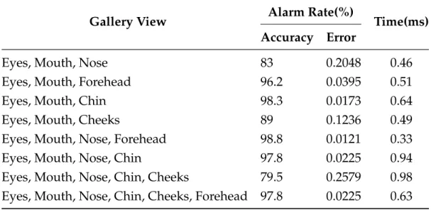
TABLE4.1: CMU-PIE face database recognition results

Gallery View Alarm Rate( % ) Time( ms ) Accuracy Error

Eyes, Mouth, Nose 96 0.0416 0.32

Eyes, Mouth, Forehead 95.4 0.0482 0.58

Eyes, Mouth, Chin 96.8 0.0331 0.74

Eyes, Mouth, Cheeks 96 0.0416 0.59

Eyes, Mouth, Nose, Forehead 97 0.0309 0.88

Eyes, Mouth, Nose, Chin 96 0.0416 0.94

Eyes, Mouth, Nose, Chin, Cheeks 97.4 0.0261 0.98 Eyes, Mouth, Nose, Chin, Cheeks, Forehead 98.4 0.0163 0.63

The results show that a combination of all face components achieves 98.4% ac-curacy. Although the accuracy varies on the different configuration of components, vigorous training of the classifier using various samples of facial components was done to ensure that the classifier could correctly classify facial components from other occluding objects that might result is misclassification. The eyes, nose and the

(46)

Chapter 4. Results and Discussion 32 forehead achieve the least recognition accuracy compared to different facial com-ponent permutations. Because some facial images of this particular database were mainly affected by hairstyle as a result, not many details were obtained from the forehead. However, other components such as the cheeks, and the chin have a lot of rich features. As a result, they achieved significantly better results compared to the other components.

4.3.2 Face Recognition under Pose Changes

The FEI face database contains images taken against a similar white background in an upright frontal position with profile rotation of up to about 180 degrees. Experi-ments on this database mainly focus on testing the pose changes with a large scale variation of up to 180◦ which is a complete full side view of the face. Table 4.2list the face recognition results of this database and it has achieved an acceptable degree of accuracy of 95.8% in an upright view with all the components combined with an error rate of 0.0163. It can be seen from the permutation of other components that all combinations achieved a recognition accuracy that is above 90%. This indicates components which are effective for facial recognition in various illumination condi-tions.

TABLE4.2: FEI face database recognition results

Gallery View Alarm Rate( % ) Time( ms ) Accuracy Error

Eyes, Mouth, Nose 93.4 0.1990 0.36

Eyes, Mouth, Forehead 93 0.0752 0.39

Eyes, Mouth, Chin 90 0.1000 0.33

Eyes, Mouth, Cheeks 93 0.0752 0.42

Eyes, Mouth, Nose, Forehead 93.4 0.0701 0.58 Eyes, Mouth, Nose, Chin 90.3 0.1074 0.63 Eyes, Mouth, Nose, Chin, Cheeks 90 0.1000 0.80 Eyes, Mouth, Nose, Chin, Cheeks, Forehead 95.8 0.0438 0.92

4.3.3 Face Recognition under Illumination Changes

Although illumination degrades the performance of the face recognition system, the contrast and brightness were achieved by preprocessing the face images using the proposed preprocessing technique discussed in section 3.2.3. In this research, the SCFace database was used to test the proposed facial recognition model under

Hybrid component-based face recognition.