Solving troesch’s problem by using modified nonlinear shooting method

(1)

78: 4–4 (2016) 45–52 | www.jurnalteknologi.utm.my | eISSN 2180–3722 |

Jurnal

Teknologi

Full Paper

SOLVING TROESCH’S PROBLEM BY USING

MODIFIED NONLINEAR SHOOTING METHOD

Norma Alias

a,

_{Abdul Manaf}

b*

_{, Akhtar Ali}

b

_{, Mustafa Habib}

c

a

_{Center for Sustainable Nanomaterials (CSNano), Ibnu Sina}

Institute for Scientific and Industrial Research, Universiti Teknologi

Malaysia, 81310 UTM Johor Bahru, Johor, Malaysia

b

_{Ibnu Sina Institute, Department of Science Mathematical, Faculty}

of Science, Universiti Teknologi Malaysia, 81310 UTM Johor Bahru,

Johor, Malaysia

c

_{Department of Mathematics, University of Engineering and}

Technology, Lahore, Pakistan

Article history Received 25 October 2015 Received in revised form

14 December 2015 Accepted 9 Febuary 2016

*Corresponding author

[email protected]

Graphical abstract

Abstract

In this research article, the non-linear shooting method is modified (MNLSM) and is considered to simulate Troesch’s sensitive problem (TSP) numerically. TSP is a 2nd_order non-linear BVP with Dirichlet boundary conditions. In MNLSM, classical 4th_order Runge-Kutta method is replaced by Adams-Bashforth-Moulton method, both for systems of ODEs. MNLSM showed to be eﬀicient and is easy for implementation. Numerical results are given to show the performance of MNLSM, compared to the exact solution and to the results by He’s polynomials. Also, discussion of results and the comparison with other applied techniques from the literature are given for TSP.

Keywords: BVPs; ODEs; predictor-corrector scheme; shooting method; Troesch’s problem

1.0 INTRODUCTION

Nowadays, Real life applications in mathematics are dealing with either an ordinary differential equations (ODE) or Partial differentials Equations (PDE). ODE is a differential equation containing a derivatives of dependent variables with respect to one independent variable. The term "ordinary" is used in contrast with the term PDE which must be with respect to more than one independent variables. Many real problems are handled with mathematical model of PDE such as Blood Flow, Solver for Breasts’ Cancerous Cell, Drying Process and laser glass cutting [1-4]. In this paper we

highlight the application of ODE which focus on Troesch’s sensitive problem (TSP).

TSP [5] is a two point 2nd_{order non-linear} boundary-value problem (TP2NLBVP) with Dirichlet boundary conditions (DBCs). TSP is defined by





sinh ( ) [0,1]; 0

with DBCs (1)

(0) 0 (1) 1

y y x and x

y and y

  

    

  

  _

TSP derived from a nonlinear system of ODEs which occurs in the confinement analysis of the plasma column via radiation pressure and also arises in the Modification of nonlinear

Shooting method

Replacement of RK with ABMM for system

Troesch’s problem

Implementation of MNLSM on TSP

Simulation by Matlab

(2)

theory of gas porous electrodes [6]. TSP has a wide range of applications in the field of applied physics.

TSP has been discussed by several researchers. Troesch [5] found solution of this sensitive problem numerically by using shooting method, while [6] used the Lie-group shooting method. Meanwhile, the authors [7] used grouping of multipoint shooting method through the assistance of continuation and perturbation technique. Besides [8] applied the quasilinearization method. In addition, other researchers applied diverse numerical techniques such as transformation groups method, invariant imbedding, and decomposition technique [9-14] for solving TSP. Meanwhile, the authors [15] discussed the solution of TSP by the inverse shooting method, [16] used the B-spline method, [17] by the sinc-Galerkin method and

[18] with the He’s Polynomials. Also, authors [19] applied the modified homotopy perturbation method, [20] used the differential transform method, [21] discussed with the chebychev collocation method and in [22] applied the sinc-collocation method. This study mainly focuses on the results of [18] obtained by using the He’s polynomials.

In this research paper, a modification of the nonlinear shooting method [23] is discussed, which is termed as a MNLSM, by substituting classical Runge-Kutta method of order four (CRKM4) by Adams-Bashforth-Moulton method (ABMM), both for systems, and is applied to find the numerical solution of TSP. MNLSM results show the complete reliability of its performance for TSP.

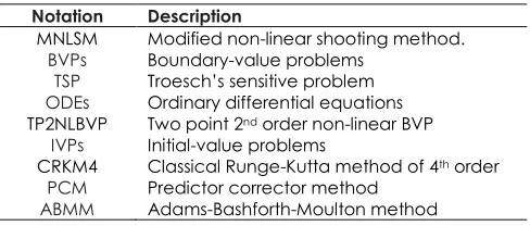
Table 1 List of abbreviations

Notation Description

MNLSM Modified non-linear shooting method.

BVPs Boundary-value problems

TSP Troesch’s sensitive problem

ODEs Ordinary differential equations TP2NLBVP Two point 2nd_{order non-linear BVP}

IVPs Initial-value problems

CRKM4 Classical Runge-Kutta method of 4th_order

PCM Predictor corrector method

ABMM Adams-Bashforth-Moulton method

2.0 MATERIALS AND METHODS

Consider the general form of a TP2NLBVP

( , ,

)

y





g x y y



with DBCs

y

( )

 

a

,

y

( )





b

(2)

Here

x





 

,



while

a b

,

are constants.

A sequence of solution in the form of IVP is obtained by choosing



as a parameter and

( , , )

y





g x y y



;

y

( )





a

and

y



( )

 



(3)

x



 



, is used to find a solution of BVP (2). Selecting

l

 



as a parameters such that

_{lim ( ,} ₎ _{( )}

k

ly

 

y



b

(4)

Here

_{y x}

_{( , )}



_l is a solution of IVP (ii) with

 



_lwhile y(x) is solution of BVP (2). This technique is called a shooting method.

Take



₀as initial elevation through which object is excited from, such that

( , ,

)

y





g x y y



;

y

( )





a

and

y



( )

 



0 (5)

If

y

( ,

 

₀

)

is not nearer to b, tried to a new elevation



1

and so on, up to

_y

_{( , )}

 

_l is perfectly close to hit b. Select parameter

l



and assume that TP2NLBVP (4) has only one solution. Let IVP (3) has a solution

y x

 

,



, then we need to find



so that

( , )

0 y

 

 

b

(6)

Newton’s method is used to find solution of this nonlinear equation. Take



₀ as an initial approximation and then generate the sequence by

₁

1

( , )

l l l

l

y b

dy d

 



 



 



  (7)

1

( ,

_l

)

dy

d



 



is needed, which is difficult to obtain

because here only values

0 1 1

( ,

), ( , ), ..., ( ,

l

)

y

 

y

 

y

 

 are available. Hence IVP (3) has to be changed such that the solution depends both on



and x [23].





( , ) , ,

(3)

To determinedy_{( , )} d



 

, when

 



_l_₁, find the

derivative of (8) w.r.t



partially.



, ( , ),

( , )



y

g

g x

g y

x y x

y x

x

y









_



_

_

 

_

 

_

 





 

Also,



and x are independent, so

x

₀





_



, then

y

_{( , )}

_x

g y

₍₉₎

y









_

 

_

 





 

From initial conditions,

( , )

0 y

_{ }









, and

( , )

1. y

_{ }











Take

U x

( , )



to indicate

y

( , )

x





and let

differentiation order of



and x is reversed. Equation (9) become IVP as

( , )

g

U x

U

y















,



 

x



;

( , )

0 U

 



and

U



( , ) 1

 



₍₁₀₎

For every single iteration, two types of IVPs obtained in the form of equations (3) and (10). Then from equation (7), 1 1 1 ( , ) ( , ) l l l l y b U

 



 

   

  (11)

Hence, in the shooting method for TP2NLBVPs, CRKM4 is applied to evaluate together the solutions essential by Newton’s method. Here ABMM as a PCM in the shooting technique for the solution of systems of IVPs is applied. PCMs also known as multistep methods, are

not self-starting, and need four initial points

( ,

x y

_i _j

); ,

i j



1, 2,3

in order to find a new point

( ,

x y

4 4

)

.

Suppose the following two 1st_{order IVPs}

1

(

1

,

1

,

1

)

j j j j

n

 



g x



n



m

 ,

n x

( )

0



n

0

1

(

1

,

1

,

1

)

j j j j

m

 

_

f x

_

n

_

m

_ ,

m x

( )

0



m

0

(12)

(13)

Applied following as a predictor formulas, which is the four step Adams Bashforth method, and apply only one time in the iteration.





1 55 59 1 37 2 9 3

24

j j j j j j

h

n  n g g  g  g (14)





1

55

59

1

37

2

9

3

24

j j j j j j

h

m

_



m



f





f



_



f



_



f



_ (15)

Applied following as a corrector formula, which is the three step Adams Moulton method, and apply this formula as many times as needed to attain the required accuracy level.





1

9

1

19

5

1 2

24

p

j j j j j j

h

n

_

 

n

g



_



g





g



_



g



_ (16)





1

9

1

19

5

1 2

24

p

j j j j j j

h

m

_



m



f



_



f





f



_



f



_ (17)

where p stands for the predicted value.

This complete procedure is known as MNLSM for the solutions of TP2NLBVPs.

3.0 RESULTS AND DISCUSSION

In this research the simulations are carried out by using Matlab and implemented on Core I7 window 8.1 system. The step size h=0.1 and error bound 10-4 _are taken for the solution of TSP (1).

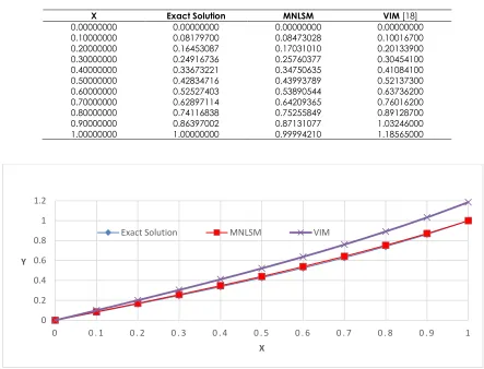
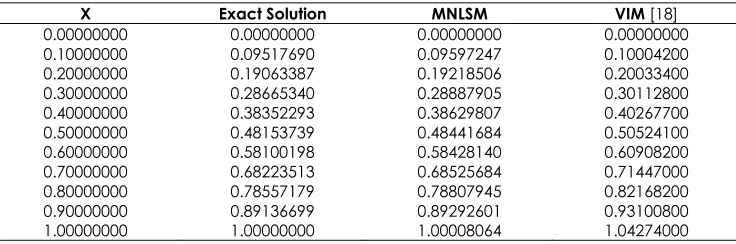
Table 2 Numerical results for TSP with



= 0.5

X Exact Solution MNLSM VIM [18]

(4)

Table 2 represents the results obtained from MNLSM when x varies from 0 to 1. The obtained results are compared with exact solution and VIM [18]. The MNLSM results are more precise than of VIM [18] for TSP with



= 0.5.

Figure 1 shows the comparison between numerical results of MNLSM and VIM [18] with the exact solution for TSP using



= 0.5. The curve of MNLSM coincides with the exact solution whereas curve of VIM [18] clearly show the difference from the exact solution.

Figure 1 Numerical results for TSP with



= 0.5

Table 3 Absolute errors for TSP with



= 0.5

x Exact Solution MNLSM VIM [18]

0.00000000 0.00000000 0.00000000 0.00000000 0.10000000 0.09517690 0.00079557 0.00486510 0.20000000 0.19063387 0.00155119 0.00970013 0.30000000 0.28665340 0.00222565 0.01447460 0.40000000 0.38352293 0.00277514 0.01915407 0.50000000 0.48153739 0.00287945 0.02370361 0.60000000 0.58100198 0.00327942 0.02808002 0.70000000 0.68223513 0.00302171 0.03223487 0.80000000 0.78557179 0.00250766 0.03611021 0.90000000 0.89136699 0.00155902 0.03964101 1.00000000 1.00000000 0.00008064 0.04274000

Results of MNLSM in Table 3 indicates that as value of x varies from 0 to 1, the absolute errors of MNLSM is not increasing faster than the absolute errors of VIM [18], when compared to the exact solution for TSP using



= 0.5.

Results of MNLSM in Table 4 indicates that as value of x varies from 0 to 1, the obtained results are more precise than of VIM [18], when compared with exact solution of TSP using



=1.

0 0.1 0.2 0.3 0.4 0.5 0.6 0.7 0.8 0.9 1

0 0 . 1 0 . 2 0 . 3 0 . 4 0 . 5 0 . 6 0 . 7 0 . 8 0 . 9 1

Y

X

(5)

Table 4 Numerical results for TSP with



= 1.

0.00000000 0.00000000 0.00000000 0.00000000 0.10000000 0.08179700 0.08473028 0.10016700 0.20000000 0.16453087 0.17031010 0.20133900 0.30000000 0.24916736 0.25760377 0.30454100 0.40000000 0.33673221 0.34750635 0.41084100 0.50000000 0.42834716 0.43993789 0.52137300 0.60000000 0.52527403 0.53890544 0.63736200 0.70000000 0.62897114 0.64209365 0.76016200 0.80000000 0.74116838 0.75255849 0.89128700 0.90000000 0.86397002 0.87131077 1.03246000 1.00000000 1.00000000 0.99994210 1.18565000



= 1

Figure 2 shows the comparison between numerical results of MNLSM and VIM [18] with the exact solution for TSP using



= 1. The curve of MNLSM coincides with

the exact solution whereas curve of VIM [18] clearly show the difference from the exact solution.



= 1

0.00000000 0.00000000 0.00000000 0.00000000 0.10000000 0.08179700 0.00293328 0.01837000 0.20000000 0.16453087 0.00577923 0.03680813 0.30000000 0.24916736 0.00843641 0.05537364 0.40000000 0.33673221 0.01077414 0.07410879 0.50000000 0.42834716 0.01159073 0.09302584 0.60000000 0.52527403 0.01363141 0.11208797 0.70000000 0.62897114 0.01312251 0.13119086 0.80000000 0.74116838 0.01139011 0.15011862 0.90000000 0.86397002 0.00734075 0.16848998 1.00000000 1.00000000 0.00005790 0.18565000

Results of MNLSM in Table 5 indicates that as value of x varies from 0 to 1, the absolute errors of MNLSM is not

increasing faster than the absolute errors of VIM [18], when compared to the exact solution for TSP using

1. 



0 0.2 0.4 0.6 0.8 1 1.2

0 0 . 1 0 . 2 0 . 3 0 . 4 0 . 5 0 . 6 0 . 7 0 . 8 0 . 9 1

Y

X

(6)

Table 6 Numerical solutions of TSP for



= 0.5

x Exact

Solution MNLSM Sinc collocation [22] Variational [14] MHP [19] Decomposition [11] 0.1000000 0.0951769 0.0959725 0.0959443 0.1000416 0.0959395 0.0959477 0.2000000 0.1906339 0.1921851 0.1921287 0.2003336 0.1921193 0.1921352 0.3000000 0.2866534 0.2888791 0.2887944 0.3011275 0.2887806 0.2888034 0.4000000 0.3835229 0.3862981 0.3861848 0.4026773 0.3861675 0.3861955 0.5000000 0.4815374 0.4844168 0.4845471 0.5052411 0.4845274 0.4845585 0.6000000 0.5810020 0.5842814 0.5841332 0.6090820 0.5841127 0.5841442 0.7000000 0.6822351 0.6852568 0.6852011 0.7144698 0.6851822 0.6852105 0.8000000 0.7855718 0.7880795 0.7880165 0.8216826 0.7880018 0.7880234 0.9000000 0.8913670 0.8929260 0.8928542 0.9310084 0.8928462 0.8928578

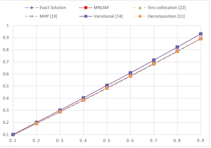
Table 6 and table 7 shows the numerical results and absolute errors of different methods from literature and their comparison with exact solution and with the MNLSM for TSP with



= 0.5.

Figure 3 shows the comparison between numerical results of different methods from literature and their comparison with exact solution and with the MNLSM for TSP with



= 0.5.



= 0.5

Table 7 Absolute errors of TSP with



= 0.5

x Exact

0.1 0.2 0.3 0.4 0.5 0.6 0.7 0.8 0.9 1

0 . 1 0 . 2 0 . 3 0 . 4 0 . 5 0 . 6 0 . 7 0 . 8 0 . 9

Exact Solution MNLSM Sinc-collocation [22]

(7)

Table 8 Numerical solutions of TSP with



= 1

x Exact

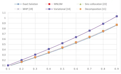
Table 8 and table 9 shows the numerical results and absolute errors of different methods from literature and their comparison with exact solution and with the MNLSM for TSP with



= 1.

Figure 4 shows the comparison between numerical results of different methods from literature and their comparison with exact solution and with the MNLSM for TSP with



= 1.



= 1



= 1

x Exact

Finally from results and discussion, it is concluded that MNLSM is superior to VIM [18] for solving Troesch’s

sensitive problem. Meanwhile, MNLSM produces good results when compared with Sinc-collocation [22],

0.1 0.2 0.3 0.4 0.5 0.6 0.7 0.8 0.9 1 1.1

0 . 1 0 . 2 0 . 3 0 . 4 0 . 5 0 . 6 0 . 7 0 . 8 0 . 9

Exact Solution MNLSM Sinc-collocation [22]

(8)

Variational [14], MHP [19] and Decomposition [11] results available in literature. Also, MNLSM is acceptable for solving others TP2NLBVPs.

4.0 CONCLUSION

The objective of this study is to modify the non-linear shooting method. The obtained MNLSM has been applied to solve TP2NLBVPs numerically with DBCs. Numerical simulations of TSP pointed out that the results attained by MNLSM are superior and close to the exact solution as compared with the results (He’s results are superior to the earlier ones. In future, higher order TSPs may be solved by using parallel computing techniques [24-26].

References

[1] Alias, N., M.R. Islam, T. Ahmad, and M.A Razzaque. 2013. Sequential Analysis of Drug Encapsulated Nanoparticle Transport and Drug Release Using Multicore Shared-memory Environment. Fourth International Conference and Workshops on Basic and Applied Sciences (4th ICOWOBAS) and Regional Annual Fundamental Science Symposium 2013 (11th RAFSS). Johor, Malaysia. 3 September 2013. 1-6.

[2] Alias, N., M.R. Islam, and N.S. Rosly. 2009. A Dynamic PDE Solver for Breasts’ Cancerous Cell Visualization on Distributed Parallel Computing Systems. 8th International Conference on Advances in Computer Science and Engineering (ACSE 2009). Phuket, Thailand. 16-18, March 2009.

[3] Alias, N., H.F.S. Saipol, and A.C.A. Ghani. 2014. Chronology of DIC Technique Based on the Fundamental Mathematical Modeling and Dehydration Impact. Journal of Food Science and Technology. 51(12): 3647-3657. [4] Alias, N., R. Shahril, M.R. Islam, N. Satam, and R. Darwis.

2008. 3D Parallel Algorithm Parabolic Equation for Simulation of the Laser Glass Cutting Using Parallel Computing Platform. The Pacific Rim Applications and Grid Middleware Assembly (PRAGMA15). Penang, Malaysia, Oct 21-24, 2008.

[5] Troesch, B. 1976. A Simple Approach to a Sensitive Two-Point Boundary Value Problem. Journal of Computational Physics. 21(3): 279-290.

[6] Hashemia, M., and S. Abbasbandyb. 2014. A Geometric Approach for Solving Troesch’s Problem. Bulletin of the Malaysian Mathematical Sciences Society.

[7] Roberts, S., and J. Shipman. 1972. Solution of Troesch's Two-Point Boundary Value Problem By A Combination Of Techniques. Journal of Computational Physics. 10(2): 232-241.

[8] Miele, A., A. Aggarwal, and J. Tietze. 1974. Solution Of Two-Point Boundary-Value Problems with Jacobian Matrix Characterized by Large Positive Eigenvalues. Journal of Computational Physics. 15(2): 117-133.

[9] Chiou, J., and T. Y. Na. 1975. On the Solution of Troesch's Nonlinear Two-Point Boundary Value Problem using an Initial Value Method. Journal of Computational Physics. 19(3): 311-316.

[10] Scott, M. R. 1974. Conversion of Boundary-Value Problems into Stable Initial-Value Problems via Several Invariant Imbedding Algorithms. Sandia Labs. Albuquerque, N. Mex. (USA).

[11] Deeba, E., S. Khuri, and S. Xie. 2000. An Algorithm for Solving Boundary Value Problems. Journal of Computational Physics. 159(2): 125-138.

[12] Khuri, S. 2003. A Numerical Algorithm for Solving Troesch's Problem. International Journal of Computer Mathematics. 80(4): 493-498.

[13] Momani, S., S. Abuasad, and Z. Odibat. 2006. Variational Iteration Method for Solving Nonlinear Boundary Value Problems. Applied Mathematics and Computation. 183(2): 1351-1358.

[14] Chang, S.H. 2010. A Variational Iteration Method for Solving Troesch’s Problem. Journal of Computational and Applied Mathematics. 234(10): 3043-3047.

[15] Snyman, J. 1979. Continuous and Discontinuous Numerical Solutions to The Troesch Problem. Journal of Computational and Applied Mathematics. 5(3): 171-175.

[16] Khuri, S., and A. Sayfy. 2011. Troesch’s Problem: A B-Spline Collocation Approach. Mathematical and Computer Modelling. 54(9): 1907-1918.

[17] Zarebnia, M., and M. Sajjadian. 2012. The Sinc–Galerkin Method for Solving Troesch’s Problem. Mathematical and Computer Modelling. 56(9): 218-228.

[18] Mohyud-Din, S. T. 2011. Solution of Troesch’s Problem using He’s Polynomials. Rev. Un. Mat. 52: 1.

[19] Feng, X., L. Mei, and G. He. 2007. An Efficient Algorithm for Solving Troesch’s Problem. Applied Mathematics and Computation. 189(1): 500-507.

[20] Chang, S.H., and I.L. Chang. 2008. A New Algorithm for Calculating One-Dimensional Differential Transform of Nonlinear Functions. Applied Mathematics and Computation. 195(2): 799-808.

[21] El-Gamel, M., and M. Sameeh. 2013. A Chebychev Collocation Method for Solving Troesch’s Problem. Int. J. Math. Comput. Appl. Res. 3: 23-32.

[22] El-Gamel, M. 2013. Numerical Solution of Troesch’s Problem by Sinc-Collocation Method. Applied Mathematics. 4(04): 707.

[23] Manaf, A., M. Habib, and M. Ahmad. 2015. Review of Numerical Schemes for Two Point Second Order Non-Linear Boundary Value Problems. Proceedings of the Pakistan Academy of Sciences. 52 (2): 151-158.

[24] Alias, N., and M. Islam, M. 2010. A Review of The Parallel Algorithms for Solving Multidimensional PDE Problems. Journal of Applied Sciences. 10(19): 2187-2197 [25] Alias, N., H.F.S. Saipol, and .A.C.A. Ghani. 2012. Numerical

method for Solving Multipoints Elliptic-Parabolic Equation for Dehydration Process. World Applied Science Journal. 21:130-135.