Sleep stage classification using hydraulic bed sensor

SLEEP STAGE CLASSIFICATION USING HYDRAULIC BED SENSOR _______________________________________

A Thesis

presented to

the Faculty of the Graduate School

at the University of Missouri-Columbia

_______________________________________________________

In Partial Fulfillment

of the Requirements for the Degree

Master of Science

_____________________________________________________ by

Ruhan Yi

James Keller, Thesis Supervisor

The undersigned, appointed by the dean of the Graduate School, have examined the thesis entitled

SLEEP STAGE CLASSIFICATION USING HYDRAULIC BED SENSOR presented by Ruhan Yi,

candidate for the degree of master of science

and hereby certify that, in their opinion, it is worthy of acceptance.

James M. Keller

Marjorie Skubic

DEDICATION

This thesis is dedicated to my parents for their endless support and encouragement.

ii

ACKNOWLEDGMENTS

I would like to express my sincere gratitude to my advisor Dr. James Keller for his patience, motivation, and continuous support of my master’s study. His guidance helped me in all the time of research and writing this thesis.

My sincere thanks also goes to Dr. Marjorie Skubic and Dr. Mihail Popescu. Thanks for providing me an opportunity to join the sleep study group and for their insightful comments.

I also want to thank my colleague, Moein Enayati, who gave me a lot of suggestions and was always willing to help.

iii

TABEL OF CONTENTS

DEDICATION

ACKNOWLEDGEMENTS ...ii

LIST OF FIGURES ... v

LIST OF TABLES ...viii

ABSTRACT ... x

CHAPTER 1. INTRODUCTION... 1

CHAPTER 2. BACKGROUND... 4

2.4 Heart Rate Variability (HRV) ... 8

2.5 Respiratory Variability (RV) ... 9

2.6 Performance measurements ... 10

2.6.1 Classifier performance measurements ... 10

2.6.2 Sleep quality measurements ... 12

2.7 Validation ... 12

2.8 Literature review ... 13

CHAPTER 3. METHODS ... 17

3.1 Data collection... 17

3.1.1 Hydraulic bed sensors ... 17

iv

3.1.3 Data synchronization... 21

3.1.4 Data collection ... 29

3.2 Signal processing ... 30

3.2.1 Bed sensor signal filtering ... 31

3.2.2 Heart beat detection... 32

3.2.3 Respiration peak detection ... 34

3.3 Feature extraction ... 35

3.3.1 Heart rate variability (HRV) features... 35

3.3.2 Respiratory Variability (RV) Features ... 40

3.3.3 Linear Frequency Cepstrum Coefficients (LFCC) features ... 44

3.4 Support vector machine (SVM) ... 47

3.5 k-nearest neighbors (k-NN) ... 49

CHAPTER 4. EXPERIMENTS ... 51

4.1 Put all subjects together ... 52

4.1.1 Single classifier ... 52

4.1.2 Hierarchical classification ... 61

4.2 Leave-one-subject-out strategy ... 64

4.2.1 Three class classifier ... 64

4.2.2 Hierarchical classification ... 69

CHAPTER 5. CONCLUSIONS ... 75

CHAPTER 6. FUTURE WORK ... 77

v

LIST OF FIGURES

Figure 1. Example of hypnogram for the entire night ... 5

Figure 2. Theoretical BCG waveform... 6

Figure 3. RJ interval of ECG and BCG signal ... 7

Figure 4. Natus SleepWorks visualization ... 8

Figure 5. Placement of four transducers under the mattress. ... 17

Figure 6. Thirty-second timelines for raw signals and filtered signals of four transducers. The top four channel timelines show the raw signals; the bottom four channel timelines show the filtered signals. ... 19

Figure 7. Hypnogram of an entire night exported from a PSG system... 20

Figure 8. Annotation of sleep study ... 21

Figure 9. Tapping motion in bed sensor signal and corresponding annotation ... 23

Figure 10. Time synchronization by aligning the "Bathroom visit" annotations ... 23

Figure 11. Aligning the data using posture changes... 24

Figure 12. Annotation example of PSG system with break ... 25

Figure 13. Example of bed sensor collecting data with subject out of bed ... 26

Figure 14. Incomplete epoch removed from PSG system ... 27

Figure 15. Incomplete epoch removed from bed sensor signal ... 27

Figure 16. Bed sensor signals with missing data ... 28

Figure 17. Corresponding data to the missing epoch in sleep stage ... 28

Figure 18. Filtered heart rate and respiration signal in 30-second epochs ... 32

Figure 19. Heart beat detection for one epoch using algorithm from[10]. The red circles at the top are the detected heartbeats ... 33

Figure 20. Heart beat location with respect to beat number for the epoch shown in Figure 19 ... 33

Figure 21. Respiratory peaks and troughs detection for the epoch shown in Figure 19. The red and blue circles are detected peaks and troughs ... 34

vi

Figure 23. Heart beat intervals for the epoch shown in Figure 19 ... 36

Figure 24. Successive difference of heart beat intervals for the epoch shown in Figure 19 ... 37

Figure 25. Heart beat intervals based on applied interpolation with 4 Hz for the epoch shown in Figure 19. (a) Before applied interpolation. (b) After applied interpolation 39 Figure 26. Power spectral density of heart beat interval for the epoch shown in Figure 19 ... 40

Figure 27. Inspiration and expiration of two different signal types in one epoch ... 42

Figure 28. Power spectrum of the first time frame for the epoch shown in Figure 19 45 Figure 29. Linear filter bank with 26 triangular filters between frequency range 0.7Hz to 10Hz ... 45

Figure 30. Twenty-six log filter bank energies of the first time frame for the epoch shown in Figure 19 ... 46

Figure 31. Twenty- five mean LFCCs along time frame for the epoch shown in Figure 19 ... 47

Figure 32. Twenty- five standard deviation LFCCs along time frame for the epoch shown in Figure 19 ... 47

Figure 33. ROC and AUC of one sleep stage regarded as positive class, other two sleep stages regarded as negative class. ... 54

Figure 34. Accuracy with different odd numbers of neighbor k ... 56

Figure 35. Kappa value with different odd numbers of neighbor k ... 56

Figure 36. Importance estimates of features ... 58

Figure 37. Features with two different importance estimates for entire night and corresponding sleep stages (0: wake; 1: REM; 2: Light; 3: Deep). (a) Feature number 50 with highest importance estimate and sleep stages. (b) Feature number 4 with least importance estimate and sleep stages. ... 58

Figure 38. Correlation graph ... 59

Figure 39. ROC curve of rem detection, AUC = 0.97 ... 61

vii

Figure 41. Average value of seventy-four features of REM stage of five subjects. ... 66 Figure 42. Average value of feature number 23 of REM stage of two subjects. ... 67 Figure 43. Four epochs of chest band signal during REM sleep of subject 0319 ... 68 Figure 44. Respiration signal filtered from bed sensor signal in REM stage of subject 0319. ... 68

viii

LIST OF TABLES

Table 1. Strength of agreement corresponding to kappa value ... 12

Table 2. Subjects with proportion of each sleep stage after preliminary selection ... 30

Table 3. Frequency band definition and frequency range ... 40

Table 4. Nineteen subjects with three sleep postures after selection ... 51

Table 5. Selected subjects with epoch number of each sleep stage ... 52

Table 6. Confusion matrix of three sleep stage classifications using cubic SVM classifier ... 53

Table 7. True positive rates and false negative rates of three sleep stage classification using cubic SVM classifier ... 53

Table 8. True positive rates and false negative rates of four sleep stage classification using cubic SVM classifier ... 55

Table 9. Selected subjects with percentage of four different sleep stages ... 55

Table 10. Confusion matrix of three sleep stage classifications using k-NN classifier ... 57

Table 11. True positive rates and false negative rates of three sleep stage classification using k-NN classifier ... 57

Table 12. Confusion matrix of three sleep stage classifications using cubic SVM with fifteen selected features... 60

Table 13. True positive rates and false negative rates of three sleep stage classification using cubic SVM with fifteen selected features ... 60

Table 14. Confusion matrix of REM detection using cubic SVM ... 60

Table 15. True positive rates and false negative rates of REM detection using cubic SVM ... 61

Table 17. Confusion matrix in first layer wake detection ... 62

Table 18. Confusion matrix in second layer wake detection ... 63 Table 19. True positive rates and false negative rates of three sleep stage classification

ix

using hierarchical method ... 63 Table 20. Confusion matrix, accuracy and kappa value for each subject using leave-one-subject-out strategy ... 65 Table 21. Confusion matrix, accuracy, and kappa value for each subject using leave-one-subject-out strategy after normalization ... 69 Table 22. Confusion matrix and accuracy of two layers for each subject using leave-one-subject-out hierarchical method. Rows are ground truth, columns are predicted stages. ... 71 Table 23. Confusion matrix, accuracy, and kappa value for each subject using leave-one-subject-out hierarchical method after normalization. Rows are ground truth, columns are predicted stages. ... 73

x

ABSTRACT

Sleep monitoring can help physicians diagnose and treat sleep disorders. Polysomnography(PSG) system is the most accurate and comprehensive method widely used in sleep labs to monitor sleep. However, it is expensive and not

comfortable, patients have to wear numerous devices on their body surface. So a non-invasive hydraulic bed sensor has been developed to monitor sleep at home.

In this thesis, the sleep stage classification problem using hydraulic bed sensor was proposed. The sleep process divided into three classes, awake, rapid eye

movement (REM) and non-rapid eye movement (NREM). The ground truth sleep stage came from regularly scheduled PSG studies conducted by a sleep-credentialed physician at the Sleep Center at the Boone Hospital Center (BHC) in Columbia, Missouri. And we were allowed to install our hydraulic bed sensors to their study protocol for consenting patients. The heart rate variability (HRV) features, respiratory rate (RV) features, and linear frequency cepstral coefficient(LFCC) were extracted from the bed sensors’ signals. In this study, two scenarios were applied, put all subjects together and leave one subject out. In each scenario, two types of

classification structures were implemented, a single classifier and a multi-layered hierarchical method. The results show both potential benefits and limitations for using the hydraulic bed sensors to classify sleep stages.

1

CHAPTER 1. INTRODUCTION

Sleep occupies a considerable part of a person’s life. Good sleep quality contributes to the repair of the human physiological and neurological systems. Insufficient sleep may increase the incidence of chronic diseases and may also threaten public safety. Sleep disorders, such as insomnia and sleep apnea, have become factors that affect people’s daily life. Studies show that the prevalence of obstructive sleep apnea (OSA) in the general population ranges from 9% to 38% and is higher in men [1]. Davies et al. [2] noted that 92% of women and 82% of men with moderate to severe OSA are undiagnosed. In addition, sleep disturbance is associated with many neurological and psychiatric diseases, such as Alzheimer’s Disease [2, 3] and Parkinson's disease [4]. Therefore, monitoring sleep and studying sleep structure is especially important.

Polysomnography(PSG) is a multi-parametric system widely used in sleep labs to diagnose and treat sleep disorders. By placing many electrodes, sensors, tubes, and masks on a patient’s body surface, the system is able to simultaneously monitor multiple biological signals, including those signals normally recorded by an electroencephalogram (EEG), electrocardiography (EKG), electrooculography (EOG), and electromyography (EMG). The conditions monitored include airflow, respiratory effort, leg movements, and oxygen saturation. Besides, a technician monitors the patient throughout the night and annotates the sleep stages based on 30-second epochs. The sleep scoring follows the American Academy of Sleep Medicine (AASM) Manual [5]. The normal sleep structure is the alternate of rapid eye movement (REM) sleep and

2

non-rapid eye movement (NREM) sleep. Furthermore, the NREM sleep from light to deep can be divided into stages NREM1, NREM2, NREM3, and NREM4. Although the PSG system has great advantages in accuracy and comprehensiveness, inevitably, it is expensive, and it can only be done by a sleep-credentialed physician in a sleep lab. In addition, wearing all the devices on the body surfaces and sleeping in a different bed in a new environment will change the patients’ sleep pattern and affect the sleep study results to some extent. In this case, widely applicable non-invasive sleep monitoring systems can greatly facilitate in-home sleep monitoring [6, 7].

A non-invasive hydraulic bed sensor has been developed to monitor sleep at home [8, 9]. No electrodes are placed on the body surface. The sensor is installed under the mattress. The system starts collecting signals as soon as a patient lies on the bed. Compared with the PSG system, it is convenient to operate and will not affect a person’s normal sleep pattern. Previous research has proposed reliable approaches to detect the heart rate and respiration rate from the hydraulic bed sensor signals [10-12]. Further, variabilities in the heart rate and respiration are also extracted. Many studies have shown high classification accuracy with these features [7, 13-15]. Therefore, the sensors’ ability to provide the features of our heart rate and respiration feedback are applied in this study.

For this thesis, the data collection took place during the regularly scheduled PSG studies conducted by a sleep-credentialed physician at the Sleep Center at the Boone Hospital Center (BHC) in Columbia, Missouri. We were allowed to install our hydraulic bed sensors to their study protocol for consenting patients. Furthermore, we

3 shared the de-identified PSG data.

In this study, two scenarios were applied—one where all the sleep study participants are together and the other where all the participants are together except for one subject, who is left out. In each scenario, two types of classification structures were implemented, a single classifier and a multi-layered hierarchical method. The support vector machine (SVM) with different types of kernels and k nearest neighbors (k-NN) with a varying number of neighbors and different distance metrics were applied. The heart rate variability (HRV) features, respiratory rate (RV) features, and linear frequency cepstral coefficient(LFCC) were extracted from the bed sensors’ signals. The results show both potential benefits and limitations for using the hydraulic bed sensors to classify sleep stages. The performance where all subjects were together was much better than the leave-one-out performance.

4

CHAPTER 2. BACKGROUND

The first terminology referencing sleep stages appeared in the 1930s. The official scoring system for staging the sleep of humans was first released in 1968 [16]. Since 2007, the American Academy of Sleep Medicine Manual (AASM, 2007) [17] has become the standard for scoring sleep stages and it also provides rules for associated events during sleep. The latest version of the manual was released in April 2018 (AASM 2018)[18] .

The AASM protocol requires sleep stage scoring in 30-second epochs. In different stages of sleep, human brainwaves, eye movements, and muscle activities show different patterns. In each 30-second epoch, after integrating all this information, the technician can classify sleep into different stages.

Normal human sleep can be divided into two main categories, REM sleep and NREM sleep. Further, from shallow to deep, the NREM sleep is divided into NREM1 (N1), NREM2 (N2), and NREM3 (N3) sleep. A normal night’s sleep cycle consists of these two types of sleep stages alternating and accompanied with awake. A hypnogram is a visual representation of the sleep process, as shown in Figure1, which shows the sleep cycle of a normal night’s sleep [19]. The sleep cycle starts with N1 and then gradually transitions to N2 and N3 before finally settling into REM. The new cycle begins by following the short duration of REM sleep. In a normal night sleep, there will be 4 to 5 cycles. As sleep progresses, the duration of REM sleep increases and N2 accounts for the majority of NREM sleep [19]. Overall, for adults REM sleep accounts

5

for about 20 to 25 percent of total sleep time and NREM accounts for 75 to 80 percent [20].

Figure 1. Example of hypnogram for the entire night

REM sleep is the stage in which our eyes move rapidly and most dreams happen. The characteristics of NREM sleep are different from N1 to N3. N1 is a transition from wake to sleep. Most sleep begins with N1, and this sleep can be easily interrupted by external noises. N2 accounts for 45 to 55 percent of NREM sleep. The duration of N2 gradually increases in the successive sleep cycle. As sleep progresses deeper, more external stimuli are needed to wake up from sleep. The N3 stage is known as slow wave sleep, and it only appears in the first few cycles.

There are many body system changes from one stage to another, such as sympathetic nerve activity, respiratory, and cardiovascular system changes [20]. All of these changes form the basis for extracting the features in the following method. 2.2 Ballistocardiography (BCG)

Ballistocardiography (BCG) is a non-invasive method that can measure body motion generated by the blood that flows out of lower heart chambers (left to right ventricles) with each heart contraction [21]. The modern BCG waveform was proposed by Isaac Starr [22] when he constructed a bed BCG measurement device. Since then, many different types of BCG measurement devices have become available, BCG

6

waveforms are similar. Figure 2 shows the theoretical BCG waveform, which represents the different phases of the heartbeat. The fiducial peak point F-G-H complex represents pre-ejection, I-J-K complex represents the ejection process, L-M-N represents the diastolic process. Peak J in BCG corresponds to the R peak in the electrocardiogram (ECG) waveform. The time interval of RJ peaks represents the time differences in the response to the electrical activation in the left and right ventricles as well as body motion caused by this activation. Figure 3 shows the RJ interval. The detection of the J peak in the BCG waveform is an important foundation for extracting the features related to the heartbeat.

7

Figure 3. RJ interval of ECG and BCG signal 2.3 Polysomnography(PSG)

Polysomnography(PSG) is a multi-parametric recording method applied in sleep labs to monitor physiological changes during sleep. It is a reliable tool for diagnosing sleep disorders, and it can also help adjust the treatment. In this study, we collected 77 subjects’ PSG data in cooperation with the BHC sleep lab. A total of 21 channel signals were collected by attaching different types of devices to the subjects. For instance, electrodes were placed on the subjects’ head measuring EEG and eye movements. Belts embedded with sensors were secured around the subjects’ chest and abdomen to monitor respiration. Snoring was recorded by a mini microphone placed close to the chin.

Sleep apnea is a sleep disorder, which can cause a person to repeatedly stop breathing during their sleep. Those diagnosed with sleep apnea are prescribed a continuous positive airway pressure (CPAP) mask or a bilevel positive airway pressure (BiPAP) mask. These two types of masks can deliver the flow of pressure to keep the wearer’s airway open during sleep. In the BHC sleep lab, a software called Natus

8

SleepWorks (Natus Medical Inc., San Carlos, CA, USA) is used to help the staff technician monitor a patient’s sleep during the night. It not only collects the PSG data but also performs a video recording. If the technicians have any uncertainty about the data, they can view the patient’s sleep video. It can provide a preliminary analysis of the collected data and can generate a report, which assists those physicians who make treatment recommendations. Figure 4 shows the 21 channels of PSG signals visualized in the Natus SleepWorks interface. The occurrence of obstructive apnea was also annotated by a technician and can be seen as the orange bar in Figure 4.

Figure 4. Natus SleepWorks visualization 2.4 Heart Rate Variability (HRV)

Numerous body systems change based on the sleep stages, which means physicians can use the monitored cardiovascular system, autonomic nervous system, or respiratory system information to determine sleep stages. Variations in heart rate controlled by the autonomic nervous system [23], and heart rate variability (HRV) can be easily acquired; thus, HRV is considered one of the characteristics which can give insight into what happens to the human body during sleep stages.

9

Two branches of the autonomic nervous system are related to sleep, the sympathetic nervous system and parasympathetic nervous system. In many circumstances, the two systems have an opposite reaction. Previous studies have demonstrated that when subjects have a deeper sleep in the NREM sleep stages, the heart rate slows down, the sympathetic nervous activity decreases from wakefulness, and parasympathetic activity gradually increases. During REM sleep, the heart rate increases, and the sympathetic nervous activity increases comparable to wakefulness [24].

Measurement of HRV in time and frequency domains are discussed in this study. The premise of calculating HRV is to detect the heart beat and successive heartbeat intervals. Details of time domain variables derived from the heartbeat intervals are discussed in Section 3.3.1.1. In the frequency domain, the power spectral density of the heartbeat interval are decomposed into specific frequency bands. Several studies demonstrate the relation between frequency bands and the autonomic nervous system [23, 25]. The low frequency band (0.04–0.15 Hz) is influenced by both sympathetic and parasympathetic systems. The high frequency band (0.15–0.40 Hz) is related to the parasympathetic nervous system. The ratio of the low frequency band and high frequency band represents the balance of the sympathetic and parasympathetic system. The HRV frequency domain’s derived process is discussed in Section 3.3.1.2.

2.5 Respiratory Variability (RV)

Numerous studies have shown that breathing regulation is significantly different between wakefulness and sleep [26-28]. Sleep is a dynamic physiologic state. At the

10

beginning of sleep, significant changes happen in the respiration control processes, particularly in REM sleep and NREM sleep. Minute ventilation represents the volume of air a person inhales or exhales in a minute. It starts to fall at the onset of sleep. During the NREM sleep, the minute ventilation shows increased regularity. The lowest level minute ventilation occurs during slow wave sleep. In comparison to NREM sleep, REM sleep is characterized by a reduced regularity, which is further reduced in minute ventilation. Therefore, RV can be considered as a characteristic that distinguishes different sleep stages.

2.6 Performance measurements

2.6.1 Classifier performance measurements

In a common classification problem, accuracy is one of the widely used performance measurements. It is expressed as the proportion of correct prediction. However, as shown in Table 2, the sleep stage data is imbalanced. The percentage of each sleep stage varies greatly. The NREM stage accounts for the largest proportion; thus, the average percentage for 33 preliminarily selected subjects in this research is 62%. The awake and REM only accounted for 21% and 17%, respectively. The problem of using accuracy in imbalanced data is that high accuracy means we classify the majority class. For sleep studies, class imbalance is a common problem. Typically, both accuracy and Cohen’s kappa coefficient are used to measure the performance of the classification. The kappa value (κ) measures the inter-rater agreement and is considered to be a more robust way to measure the agreement [29, 30]. In this thesis, the agreement of ground truth and predicted results were calculated in each experiment.

11

The formulas of accuracy and kappa value are described as follows: The confusion matrix is defined as:

Predicted Class

Class1 Class2

Actual Class

Class1 True Positive(TP) False Negative(FN) Class2 False Positive(FP) True Negative(TN) The accuracy is defined as:

Accuracy = 𝑇𝑃+𝑇𝑁

𝑇𝑃+𝐹𝑁+𝐹𝑃+𝑇𝑁 (2-1)

The kappa value is defined as:

κ = 𝑝0−𝑝𝑒 1−𝑝𝑒 (2-2) where 𝑝₀ = 𝑇𝑃+𝑇𝑁 𝑇𝑃+𝐹𝑁+𝐹𝑃+𝑇𝑁 (2-3) 𝑝𝑒 = (𝑇𝑃+𝐹𝑁)∗(𝑇𝑃+𝐹𝑃)+(𝐹𝑃+𝑇𝑁)∗(𝐹𝑁+𝑇𝑁) (𝑇𝑃+𝐹𝑁+𝐹𝑃+𝑇𝑁)2 (2-4)

where 𝑝₀ = 𝐴𝑐𝑐𝑢𝑟𝑎𝑐𝑦 and represents the observed agreement between two classes.

𝑝_𝑒 represents the probability of chance agreement.

The following table shows the agreement guidelines proposed in [31]. The strength of the agreement assigned to the specific range of kappa value.

12

Table 1. Strength of agreement corresponding to kappa value Kappa Strength of Agreement

< 0.00 Poor 0.01-0.20 Slight 0.21-0.40 Fair 0.41-0.60 Moderate 0.61-0.80 Substantial 0.81-1.00 Almost Perfect 2.6.2 Sleep quality measurements

In order to measure sleep quality, we may use [32]:

 Sleep efficiency (SE): The ratio of total sleep time and total time in bed.

 Percentage of REM sleep (SR): The ratio of time spent in REM sleep and total sleep time.

2.7 Validation

Here, we used two cross-validation scenarios to validate our classifiers. The first scenario is referred to as the 10-fold cross-validation. We put all the epochs of selected subjects together and partitioned the data into 10 equal sized subsets. Each time we used this validation method, one of the subsets was selected as the validation set for testing the model, and the remaining nine subsets were used for training the model. We repeated this approach 10 times and determined the accuracy by averaging the results. The benefit of this approach lies in the accuracy of its ability to evaluate the performance of the model’s features.

13

the purpose of designing a sleep stage classification system is to recognize the sleep stage of a new individual using existing data, this method has a more practical

meaning. Each time we used this validation method, we selected one subject’s data to use for testing. The remaining subjects’ data were used for training the classifier. The system was designed to have robust performance results on the chosen subjects. 2.8 Literature review

Previous studies have reported sleep stage classification results under different conditions. The data can be obtained through a PSG system, bed sensor, radar system, and a watch-based device. The quality of the signal is quite different for these

systems. Another factor is the subjects who participated in these studies. Most studies recruit healthy young adults; thus, when comparing the healthy participants to those subjects with a sleep disorder, the signal quality is much better. In this section, we compare classification results in literature.

Jialei Yang presented a sleep-stage classification method using bed sensors in her thesis [33]. Her data were collected from same healthy young subject for eight entire nights. Two scenarios were implemented for validation in the experiments. The first scenario put all the recordings together and used the 10-fold cross-validation. The best results for detecting REM were a 93% accuracy and a 0.78 kappa value obtained by using smoothed linear frequency cepstral coefficients (LFCC). For the three-stage classification, the accuracy was 81% with a 0.70 for kappa value. The three-stage classification results were better than most results for this type of test in the literature. The second scenario, the leave-one-night out method, removed one entire night’s

14

testing data; the remaining nights were used for training. The REM detection accuracy and kappa value degraded significantly, at 62% and 0.09, respectively. Such a kappa value can be regarded as a random guess for classification. For the REM and awake stages together versus NREM, the results were worse. The accuracy decreased by 50% as did the negative kappa value, which means the classification results were worse than random guessing.

Park et al. [7] showed three threshold comparison experiments detecting sleep stages by using heart rate variability parameters derived from the BCG signal. The experiment detecting the awake epoch was based on the heart rate variation threshold. The result for normal subjects was 97.4% in accuracy with a 0.83 kappa coefficient. The result for the subjects with obstructive sleep apnea was 96% in accuracy with a 0.81 kappa coefficient. The experiment for detecting REM sleep compared three heart rate parameters with the threshold. If all of the parameters were higher than their corresponding thresholds, the epoch was labeled as REM. The accuracy of 92% with a 0.72 kappa coefficient for five normal subjects was reported. The third experiment was set up to detect deep sleep. Four HRV parameters from the time domain and frequency domain were selected; thus, all of the parameters lower than the threshold in the epoch regarded as deep sleep. The results showed 89.4% in accuracy with a 0.48 kappa coefficient. After detecting the awakening, REM, and deep sleep, the remaining tests were classified as light sleep epochs. The accuracy was 76.2%, and the kappa value was 0.53.

15

based on EEG signals. The subjects in this paper were separated into two group. The subjects in one group experienced low apnea events during their sleep. The subjects in another group experienced high apnea events. A number of heart rate and respiratory rate features were extracted. A subject-specified classifier yielded 79% accuracy. When a similar subject-independent classifier was trained, the accuracy dropped to 67%. For a comparison trained classifier with EEG features, the accuracy for a subject-specified classifier was 87%. The accuracy for the subject-independent classifier was 84%.

Kortelainen et al. [6] proposed a three-stage classification system using the Emfit bed sensors (Emfit Ltd., Vaajakoski, Finland). The bed sensors obtained heart beat intervals and movements during the user’s sleep. A time-variant autoregressive model (TVAM) was used for extracting the features. A hidden Markov model (HMM) was used for training. Eighteen healthy subjects participated in the experiment. The system obtained 79% accuracy with a kappa value of 0.44.

Huang et al. [35] presented an automatic four-stage classification system with a hierarchical structure using forehead EEG signals. The hierarchical structure

consists of five layers—the preliminary wake detection layer, three SVM classifier layers, and a final fifth layer with two adaptive adjustment schemes. Ten healthy subjects were involved in this study. The accuracy was about 77% with a kappa value of 0.67. A similar hierarchical structure was implemented in one of the experiments in this study.

16

similar purpose of using non-invasive method to classify the sleep stages in this thesis. Two of them had health subjects participated in the studies. The accuracy range from 76% to 81% were obtained in three-stage classification. The same features in Jialei’s work were applied in this thesis, and obtained 85% accuracy. The accuracy for detecting REM was around 92% for healthy subjects were reported in Jialei’s and Parks’s works. Since the sleep data is imbalanced, NREM and wake together

accounted for majority of the sleep stage. The high accuracy in detecting NREM and wake may contribute to accuracy of REM detection. In Jialei’s thesis, 86% of true positive rate of REM was reported, which indicates REM was correctly classified as REM. However, Park did not show the confusion matrix or true positive rate of REM detection, so it is impossible to know the details. All of the studies show the potential of applying non-invasive sensor to build an automatic sleep stage classification system.

Only in Jialei’s work the leave-one-night-out strategy was mentioned. The data were collected from same person for 8 nights. Although they are eight separate nights, it is still different from collecting the data from eight different people. The accuracy of 63% and 45% of true positive rate in detecting REM indicated that even the data collected from same person have different characteristic from night to night. In this thesis, the results from using this strategy were not satisfactory. So, using a leave-one-subject-out strategy in sleep studies, remains a challenging problem.

17

CHAPTER 3. METHODS

3.1.1 Hydraulic bed sensors

The noninvasive hydraulic bed sensor system consists of four hydraulic bed transducers made of a flat hose partially filled with water. An integrated pressure sensor is connected to one end of each transducer. The pressure sensors can convert the weight placed on the surface into the voltage signal. These sensors are also sensitive to low amplitude variations, which makes it possible to detect a heartbeat [36].

The position of the four transducers is shown in Figure 5. To capture the heartbeat and respiration, the transducers were placed under the mattress of each bed with the same separation distance between each transducer and parallel to the direction in which the patient lies on the bed. The incline degree of each bed in the Boone Hospital Center’s sleep lab is adjustable by the patient.

Figure 5. Placement of four transducers under the mattress.

The transducers were placed above the bending part of the bed to avoid folding when the patient changes the incline degree. Each transducer has two output channels: one for raw data and another for filtered signal. An 741 op-amp amplifier was applied to serve the hardware filtering circuit, and an 8th-order integrated Bessel filter was used

18

for filtering the noise [9]. Finally, the filtered signal was sampled at 100 Hz. The details of the bed sensor construction, hardware filtering, and refinement are described in previous work [9].

Figure 6 shows a 30-second timelines for the four channels in response to the raw signals and the filtered signal of the bed sensors with one patient lying on the bed.

In the feature extraction process, for each epoch only one transducer was selected. The selection criteria in this study is based on maximum DC value. We assumed that large DC value represents more weight on the transducer and a better connection with subjects.

19

Figure 6. Thirty-second timelines for raw signals and filtered signals of four transducers. The top four channel timelines show the raw signals; the bottom four channel timelines show the filtered

20 3.1.2 Boone Hospital Center (BHC) sleep lab data

As described in Section 2.3, the BHC sleep lab provided de-identified

polysomnography (PSG) data. Different from bed sensor data, the sampling rate of all the PSG signal is 256 Hz. In addition, the annotations of sleep technician-recorded valuable information is essential to the success of this study. Aside from setting the tests up and preparing the patient for the tests, a sleep technician scores each patient’s clinical events (e.g., respiratory and cardiac events, limb movements, and arousals) using the American Academy of Sleep Medicine (AASM) standards [37].

Hypnogram is a form of PSG; it shows the sleep stages as a function of time. Figure 7 is a hypnogram presented in the NatusNeuroWorks®/SleepWorks interface [38]. Each sleep stage is annotated in 30-second epochs. From top to bottom, the sleep stages are the wake, REM, NREM1, NREM2, and NREM3. For this patient, 742 epochs were monitored during sleep. REM sleep happened between epoch 392 and epoch 485.

Figure 7. Hypnogram of an entire night exported from a PSG system

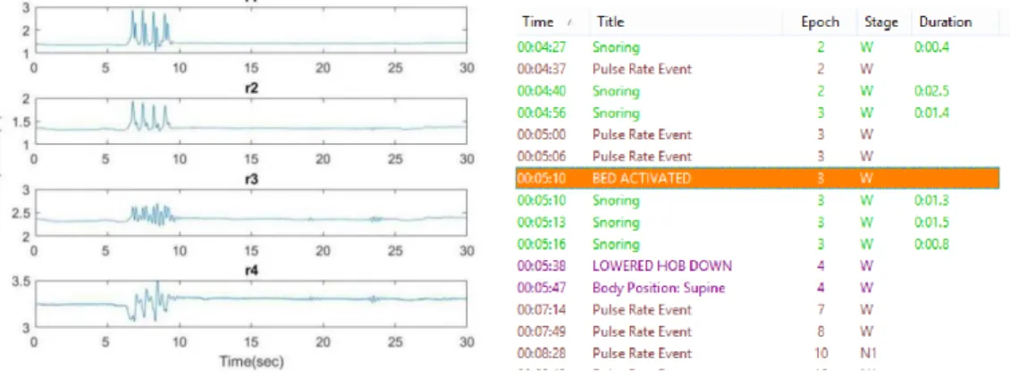
Figure 8 shows the example of an annotation displayed on the interface, which recorded all of the sleeper’s events during the sleep study. These events include the time, title, and duration of an event, and corresponding sleep stage and epoch. In this example we can see that the patient changed body position to supine, and then changed to left. There will be some movement artifacts along with the change of body position. Movement artifact is generated by movement of cables or electrodes when patients

21

move normally in sleep. It usually solves itself when the patient stops moving. The technician should ensure that the electrodes are not displaced after the patient stops moving [39]. If there is still an artifact, the technician must repair the electrodes.

Figure 8. Annotation of sleep study

By exporting all the signals and annotations, we were able to obtain the comprehensive information and ground truth needed for our sleep study.

3.1.3 Data synchronization 3.1.3.1 Start time synchronization

As previously mentioned, to protect the privacy of patients participating in this experiment, all the data collected from the sleep lab was de-identified. We are not able to identify the subjects by their name. Furthermore, no matter when the data collection begins, the time stamp for the annotation starts at midnight (00:00:00). Since we collected the data using two independent systems simultaneously, we know the accurate

22

time stamp of the bed sensor system. Synchronizing the two system became an issue. We used two approaches to solve this issue. One approach is based on sudden variations in the signal of the two systems. This procedure was done with help of technicians in the sleep lab. After every test, all the devices were working properly. If the technician taps on a mattress three times, this action will be recorded in the annotation as an “active bed sensor.”

The synchronization approach is to find the time stamp when the “three taps” occurred in the bed sensor signal, and then synchronize it with the time in which the “active bed sensor” became a part of the sleep lab annotation. Figure 9 is an example of the procedure where (a) shows the tapping action occurring at 22:22:25 in the bed sensor signal, and (b) shows the tapping action occurring at 00:05:10 in the de-identified annotation. In fact, the two time stamps represent the same moment in the two systems. This approach depends on signal variation at the beginning of the sleep study. At this time, the patient had just laid down on the bed, generating many movements and noise. Thus, it was difficult to distinguish the tapping action from the other noisy signals.

23

Figure 9. Tapping motion in bed sensor signal and corresponding annotation

The second approach depends on the entire night’s signals, aligning the motion annotation to the corresponding events occurring in the bed sensor signals. Figure 10 shows one of the alignment approaches based on “bathroom visit” annotation with the rapid decrease average DC value of the bed sensor data.

Obviously, the bed sensor signals generated by weight pressure on the sensors when the patient gets out of the bed caused the sensors to capture the weight changes and decrease rapidly.

Figure 10. Time synchronization by aligning the "Bathroom visit" annotations to the "Low DC value" of the bed sensor.

24

subject that did not get out of the bed for the entire night. In this case, we use posture changes to align the data. The changes in the bed sensor signal does not always match the posture changes. For example, the first DC value change happened around 01:20 am, the posture also changed around that time. However, the third DC value change happened around 01:40 am, there is a delay in posture change.

Figure 11. Aligning the data using posture changes

Since both approaches are not applicable in some situations, we alternately applied two approaches to improve the synchronization accuracy.

3.1.3.2 Break time synchronization

Although we synchronized the starting time of two systems, there were some interruptions during the sleep. Forty-seven out of 77 patients went to the restroom during the study. The number of restroom visits varied from one to five times. When a patient gets out of the bed, the technician has to disconnect all the devices worn on that person’s body surface and interrupt the PSG data collection. At the same time, the bed sensors are supposed to stop collecting the data.

The first interruption to the flow of signals was when the subjects got out of bed but the bed sensors kept on collecting data. Figure 12 shows an annotation example of

25

the PSG system with the epoch number labeled at the top left of the beginning of each epoch. As can be seen in the figure, during epoch 55 the system was disconnected, and then reconnected during epoch 62.

Figure 12. Annotation example of PSG system with break

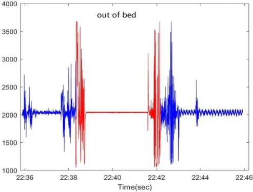
According to the results of data synchronization, the restroom visit timestamp in the bed sensor system is from 22:38:19 to 22:42:10. However, due to a hardware malfunction, from Figure 13 we can see that the bed sensors kept on collecting data while the patient was away from the bed.

26

Figure 13. Example of bed sensor collecting data with subject out of bed

Since sleep stage is based on 30-second epochs, we don’t want to keep incomplete sleep stages. In the PSG system we look for complete epochs before the disconnected time point. In this example, the complete epoch before disconnection is epoch 54, and the complete epoch after the reconnected time point is epoch 63. The incomplete epochs with the yellow background in Figure 14 were removed. For the bed sensor system, we removed all the data between epoch 54 and epoch 63 as shown in Figure 15. The remaining signals are the integral multiple segments of 30-second epochs. We then concatenated all the signals together.

27

Figure 14. Incomplete epoch removed from PSG system

Figure 15. Incomplete epoch removed from bed sensor signal

The second exception was caused by a hardware malfunction. The bed sensor missed some part of the data, even when the patient was on his or her bed. Figure 16 is an example of this problem. According to this annotation, a patient was out of bed for about six minutes; however, there was an interval of about 13 minutes between the patient’s out of bed time and the time signals could be converted to data. For some

28

hardware reason, the bed sensors experienced a seven-minute delay before they could start collecting data again.

Figure 16. Bed sensor signals with missing data

However, in the PSG system, sleep stages were labeled during this time period. The synchronization process was much like the previous one, and the complete epoch was found to be coincident with the timestamp data. Then, the sleep stage labels were removed, which matched the missing data. Figure 17 shows the corresponding sleep stage data. Epoch 820 to epoch 845 had to be removed from the sleep stage label.

29 3.1.4 Data collection

Seventy-seven subjects (50 males, 27 females; mean age 62.8±11.4 years) participated in the sleep study. Thirty-seven of the records for these patients were removed due to poor sleep quality, such as no REM sleep or staying awake for the entire night. Some were removed because the patients wore a pacemaker which can affect heartbeat detection. Other records were removed due to patients sleeping in the wrong position, e.g., sleeping with their head on the other side of the bed.

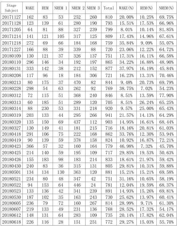
Those who participated in the sleep study had been diagnosed with a possible sleep disorder. The complete collapse and partial collapse of the airway are called apnea and hypopnea, respectively. The absence of airflow will affect breathing patterns and then influence sleep stage classification. It is necessary to remove patients with serious symptoms. The Apnea-hypopnea index (AHI) represents the number of apnea and hypopnea events per hour during the sleep. According to the AASM, the mild sleep apnea AHI is between 5 and 15. Based on the AHI provided by the PSG diagnostic report exported from NatusNeuroWorks®/SleepWorks, we eliminated seven other subjects that had an AHI higher than 15. Table 2 shows 33 subjects after preliminary selection. An epoch number is given for each sleep stage representing each subject.

30

Table 2. Subjects with proportion of each sleep stage after preliminary selection Stage

Subject WAKE REM NREM 1 NREM 2 NREM 3 Total WAKE(%) REM(%) NREM(%)

20171127 162 83 53 252 260 810 20.00% 10.25% 69.75% 20171128 123 139 61 280 190 793 15.51% 17.53% 66.96% 20171205 64 81 88 327 239 799 8.01% 10.14% 81.85% 20171214 141 121 105 317 125 809 17.43% 14.96% 67.61% 20171218 272 69 66 184 168 759 35.84% 9.09% 55.07% 20171227 166 88 39 339 88 720 23.06% 12.22% 64.72% 20180109 130 121 37 326 137 751 17.31% 16.11% 66.58% 20180110 296 146 34 192 197 865 34.22% 16.88% 48.90% 20180131 333 142 38 212 152 877 37.97% 16.19% 45.84% 20180208 117 96 18 184 306 721 16.23% 13.31% 70.46% 20180213 80 175 37 470 82 844 9.48% 20.73% 69.79% 20180228 298 54 63 262 92 769 38.75% 7.02% 54.23% 20180312 72 115 51 368 240 846 8.51% 13.59% 77.90% 20180313 60 185 51 289 120 705 8.51% 26.24% 65.25% 20180314 88 230 53 331 218 920 9.57% 25.00% 65.43% 20180319 203 133 44 295 266 941 21.57% 14.13% 64.29% 20180320 135 150 69 437 112 903 14.95% 16.61% 68.44% 20180327 130 149 41 181 215 716 18.16% 20.81% 61.03% 20180418 291 106 75 222 168 862 33.76% 12.30% 53.94% 20180419 90 139 59 378 158 824 10.92% 16.87% 72.21% 20180423 366 57 32 160 164 779 46.98% 7.32% 45.70% 20180425 214 140 59 195 109 717 29.85% 19.53% 50.63% 20180426 155 183 98 183 214 833 18.61% 21.97% 59.42% 20180430 240 83 36 315 131 805 29.81% 10.31% 59.88% 20180501 134 134 130 363 120 881 15.21% 15.21% 69.58% 20180521 234 80 48 347 42 751 31.16% 10.65% 58.19% 20180522 94 153 64 446 24 781 12.04% 19.59% 68.37% 20180523 133 136 42 341 239 891 14.93% 15.26% 69.81% 20180530 187 102 35 163 243 730 25.62% 13.97% 60.41% 20180605 236 79 72 160 267 814 28.99% 9.71% 61.30% 20180607 219 133 49 231 136 768 28.52% 17.32% 54.17% 20180612 148 131 64 283 109 735 20.14% 17.82% 62.04% 20180618 226 116 28 151 251 772 29.27% 15.03% 55.70% 3.2 Signal processing

Although the bed sensor has built-in hardware filtering, the filtered signal is still far from being ready to use in our experiment. In this section, a further filtering method

31

is proposed to separate the heart rate and the respiration signal. 3.2.1 Bed sensor signal filtering

As shown in Section 3.1.1, each channel of hardware filtered BCG consists of heartbeats, respiration, and noise. For the purpose of extracting the HRV and RV features, further filtering was applied to the hardware-filtered BCG signal to separately obtain a clean heart rate and respiration signal.

The Butterworth bandpass filter of the 6th order was implemented in this work [10]. The normal respiration rate was lower than 0.5 Hz. The filter with a cutoff range from 0.7 Hz to 10 Hz removed most of the low-frequency respiration components. So, the higher frequency heart rate component was retained.

In order to remove the high-frequency heart rate component, a low pass 6th order Butterworth filter with a cutoff frequency of 0.7 Hz was run on hardware filtered BCG [12]. Figure 18 is an example of a filtered heart rate and respiration signal in 30-second epochs.

32

Figure 18. Filtered heart rate and respiration signal in 30-second epochs 3.2.2 Heart beat detection

In Section 3.2.1, the heart rate signal was separated from the BCG signal. An algorithm proposed in [10] was implemented in this experiment to detect the heart beat. For each 30-second epoch, the algorithm detects the heart beat based on an energy of 0.3 seconds in a moving window. The red circles above the signal in Figure 19 are the heartbeat detection results of a 30-second epoch. For this subject, 36 heart beats were detected in one epoch.

The normal heart rate range is between 60 and 100 bpm. Since the bed sensor is sensitive to body movement, much noise overlaps the BCG signal. This results in an inaccurate detection of beats. Therefore, any epoch with heart rates less than 40 bpm or larger than 150 bpm was removed.

33

Figure 19. Heart beat detection for one epoch using algorithm from[10]. The red circles at the top are the detected heartbeats

If we define x(n) as the time stamp of heart beats in a 30-second epoch, and n is the number of beats, Figure 20 shows the beat locations with respect to beat number. A nearly straight line indicates the subject’s heart beat in this epoch is regular.

34 3.2.3 Respiration peak detection

In Section 3.2.1, the respiratory signal is separated from the heart beat signal. The peaks and troughs of the respiratory signal can be detected easily. Respiratory peaks and troughs detection for one epoch signal is shown in Figure 21. The red and blue circles are detected peaks and troughs respectively.

Figure 21. Respiratory peaks and troughs detection for the epoch shown in Figure 19. The red and blue circles are detected peaks and troughs

For the respiration signal, default peaks and troughs appear between each other which means exhalation and inhalation appear between each other. There are different types of exceptions in the respiration signal. Figure 22 shows one of the exceptions where two successive troughs are detected due to the shallow breath between two normal breaths. So, we find a peak between two troughs and insert the peak between them.

35

Figure 22. Insert one peak between two successive troughs 3.3 Feature extraction

3.3.1 Heart rate variability (HRV) features

After the signal processing step, heart beat locations were obtained to further determine the HRV feature and heart beat intervals (HBI). The heart beat interval is defined as the difference in successive heart beats from their location:

𝐼(𝑛) = 𝑥(𝑛 + 1) − 𝑥(𝑛) 𝑛 = 1, 2, 3 … (3-1)

Figure 23 plots the heart beat intervals corresponding to the heart beat detection shown in Figure 19.

36

Figure 23. Heart beat intervals for the epoch shown in Figure 19

The difference in successive beat-to-beat intervals is defined as:

𝐷(𝑛) = 𝐼(𝑛 + 1) − 𝐼(𝑛) 𝑛 = 1, 2, 3 … (3-2) Figure 24 plots the differences in successive beat-to-beat intervals corresponding to the heart beat intervals shown in Figure 23. Point number 8 to number 25 are around zero, which mean heart rate in this time period is stable.

37

Figure 24. Successive difference of heart beat intervals for the epoch shown in Figure 19

HRV features can be derived from two different domains, the time domain and frequency domain.

3.3.1.1 Time domain HRV features

Time domain HRV features are the statistical measures derived from the heart beat intervals and differences in successive heart beats intervals. The definition and formula are as follow:

 Square root of the mean of the squares for successive difference in interval can be calculated as

RMSSD = √∑𝑁𝑛=1𝐷(𝑛)2

𝑁 (3-3)

 The percentage of successive difference in interval > 50 ms is given as

PNN50 = P(|D(n)| > 50ms) (3-4) Where P means percentage.

 Mean of heart beat intervals is expressed as mHBI = ∑𝑁𝑛=1𝐼(𝑛)

38

 Standard deviation of successive difference of beat-to-beat intervals is written as

SDSD = √ 1 𝑁−1∑ |𝐷(𝑛) − 𝜇| 2 𝑁 𝑛=1 (3-6) μ = ∑𝑁𝑛=1𝐷(𝑛) 𝑁 (3-7)

 Standard deviation of beat-to-beat intervals is shown as

SDNN = √ 1

𝑁−1∑ |𝐼(𝑛) − 𝑚𝐻𝐵𝐼| 2 𝑁

𝑛=1 (3-8)

 Maximum of beat-to-beat intervals is written as

maxHBI = _{1≤𝑛≤𝑁}𝑚𝑎𝑥𝐼(𝑛) (3-9)

 Minimum of beat-to-beat intervals is given as

minHBI = _{1≤𝑛≤𝑁}𝑚𝐼𝑁𝐼(𝑛) (3-10)

 Differences in maximum of beat-to-beat interval and minimum of beat to beat interval are shown as

max_minHBI = _{1≤𝑛≤𝑁}𝑚𝑎𝑥𝐼(𝑛)−_{1≤𝑛≤𝑁}𝑚𝑖𝑛𝐼(𝑛) (3-11)

 Coefficient of variance is expressed as

CV = 𝑆𝐷𝑁𝑁

𝑚𝐻𝐵𝐼 (3-12)

3.3.1.2 Frequency domain HRV features

As mentioned before, the different frequency bands are related to parasympathetic and sympathetic nervous system activity. Moreover, the nervous system’s active levels change during the different sleep stages. The frequency measures of the HBI series can be used to indicate the sleep stages.

39

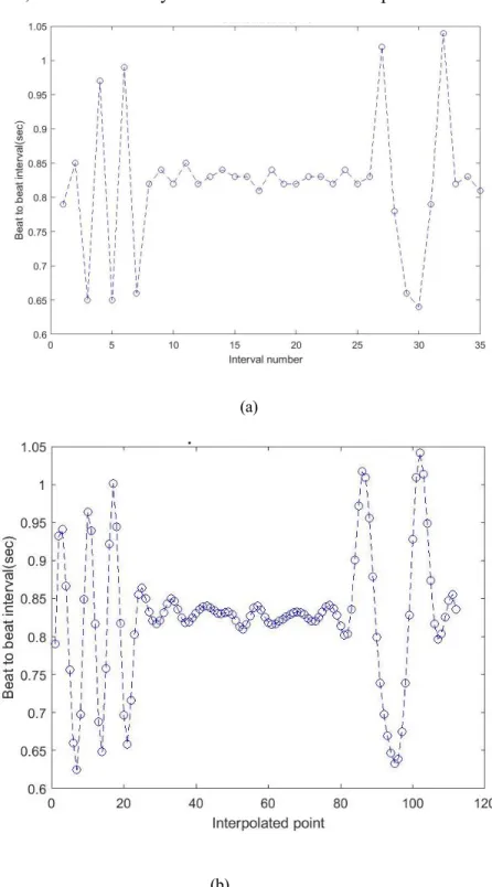
with 4 Hz was applied on the unevenly-spaced HBI. Figure 25.(a) shows the original beat to beat interval from the result in (3-1). Figure 25.(b) shows the interpolated HBI and the data points, which are evenly distributed in 30-second epochs.

(a)

(b)

Figure 25. Heart beat intervals based on applied interpolation with 4 Hz for the epoch shown in Figure 19. (a) Before applied interpolation. (b) After applied interpolation

40

The next step is to compute the PSD of HBI for each epoch using discrete Fourier transform (DFT) with 256 sampling points. Figure 26 is the corresponding PSD of HBI in Figure 23.

Figure 26. Power spectral density of heart beat interval for the epoch shown in Figure 19

The frequency band definition and frequency range are given in Table 3. Table 3. Frequency band definition and frequency range

Frequency measures Frequency range

Low frequency band(LF) 0.04-0.15Hz

High frequency band(HF) 0.15-0.4Hz

Total power(TF) 0-0.4Hz

Ratio of low frequency and high frequency: LF/HF

3.3.2 Respiratory Variability (RV) Features

In Section 3.2.3 the respiration signal peaks and troughs detection were

41

as the RV features were extracted from the breath-to-breath interval and from the successive differences of breath-to-breath intervals. The breath-to-breath intervals were defined as peak-to-peak intervals in this experiment. The time stamp of peak is x(n) and the breath-to-breath intervals are defined as:

𝐼(𝑛) = 𝑥_𝑝(𝑛 + 1) − 𝑥_𝑝(𝑛) 𝑛 = 1, 2, 3 … (3-13) and the successive differences of breath-to-breath intervals are defined as:

𝐷(𝑛) = 𝐼(𝑛 + 1) − 𝐼(𝑛) 𝑛 = 1, 2, 3 … (3-14) Different from HRV features, the respiration process can be divided into two parts, expiration and inspiration. The expiration is defined as trough-to-peak and the inspiration is defined as peak-to-trough. and represent the interval of inspiration and expiration. and represent the differences between the inspiration and expiration amplitude. The signal of each 30-second epoch can be divided into two types, the signal beginning with inspiration and the signal beginning with expiration.

If the signal begins with inspiration as shown in Figure 27(a), the inspiration and expiration intervals are defined as:

𝐼_𝑖(𝑛) = 𝑥_𝑡(𝑛) − 𝑥_𝑝(𝑛) 𝑛 = 1, 2, 3 … (3-15) 𝐼𝑒(𝑛) = 𝑥𝑝(𝑛) − 𝑥𝑡(𝑛) 𝑛 = 1, 2, 3 … (3-16) The difference of the amplitudes are defined as:

𝐴𝑒(𝑛) = 𝐴𝑝(𝑛 + 1) − 𝐴𝑡(𝑛) 𝑛 = 1, 2, 3 … (3-17) 𝐴_𝑖(𝑛) = 𝐴_𝑝(𝑛) − 𝐴_𝑡(𝑛) 𝑛 = 1, 2, 3 … (3-18) ) ( i n I I_e(n) ) ( i n A A_e(n)

42

(a) (b)

Figure 27. Inspiration and expiration of two different signal types in one epoch

If the signal begins with expiration as shown in Figure 27(b), the inspiration and expiration intervals are defined as:

𝐼_𝑒(𝑛) = 𝑥_𝑝(𝑛) − 𝑥_𝑡(𝑛) 𝑛 = 1, 2, 3 … (3-19) 𝐼_𝑖(𝑛) = 𝑥_𝑡(𝑛 + 1) − 𝑥_𝑝(𝑛) 𝑛 = 1, 2, 3 … (3-20) The differences of the amplitudes are defined as:

𝐴𝑒(𝑛) = 𝐴𝑝(𝑛) − 𝐴𝑡(𝑛) 𝑛 = 1, 2, 3 … (3-21) 𝐴𝑖(𝑛) = 𝐴𝑝(𝑛) − 𝐴𝑡(𝑛 + 1) 𝑛 = 1, 2, 3 … (3-22)

The RV features extracted from breath-to-breath intervals, successive differences of intervals, and intervals of inspiration and expiration are listed as follows:

 The square root of the mean of the squares of successive differences of breath-to-breath intervals is calculated as

RMSSD = √∑𝑁𝑛=1𝐷(𝑛)2

43

 The mean of successive differences of breath-to-breath intervals is expressed as

𝑚𝐷𝐼 = ∑𝑁𝑛=1𝐷(𝑛)

𝑁 (3-24)

 The max of the absolute differences of breath-to-breath intervals is defined as 𝑀𝐴𝐷𝐼 = _{1≤𝑛≤𝑁}𝑚𝑎𝑥|𝐷(𝑛)| (3-25)

 The mean of respiratory rate can be found by 𝑚𝑅𝑅 = 60 𝑁 ∑ 1 𝐼(𝑛) 𝑁 𝑛=1 (3-26)

 The standard deviation of respiratory rates is given as SDRR = √_𝑁−11 ∑ | 60

𝐼(𝑛)− 𝑚𝑅𝑅| 2 𝑁

𝑛=1 (3-27)

 The coefficient of variance is defined as CV = 𝑆𝐷𝑅𝑅

𝑚𝑅𝑅 (3-28)

 The median of respiratory rate is written as MedianRR = 𝑄2(

60

𝐼(𝑛)) (3-29) Where 𝑄2 means median

 The inter quartile range of respiratory rate can be found by the following calculation: IQR = 𝑄3( 60 𝐼(𝑛)) − 𝑄1( 60 𝐼(𝑛)) (3-30) Where 𝑄1 and 𝑄3 are the first quartile and the third quartile respectively.

 The mean of the absolute deviation value of respiratory rates is expressed as MAD = 1 𝑁∑ | 60 𝐼(𝑛)− 𝑚𝑅𝑅| 𝑁 𝑛=1 (3-31)

44 inspiration

∑𝑁𝑛=1𝐴𝑒(𝑛) ∑𝑁𝑛=1𝐴𝑖(𝑛)

(3-32)

 The ratio of mean of expiration intervals and inspiration intervals are defined as ∑𝑁𝑛=1𝐼𝑒(𝑛)

∑𝑁𝑛=1𝐼𝑖(𝑛)

(3-32)

3.3.3 Linear Frequency Cepstrum Coefficients (LFCC) features

The cepstrum is the result of an inverse Fourier transform of the logarithm of the signal spectrum. The mel frequency cepstral coefficient (MFCC) is defined as the real cepstrum of a windowed signal derived from FFT of the signal [40], and it has been widely used in voice recognition algorithms [41]. In some sleep studies, linear frequency cepstrum coefficients (LFCC) have been used to solve sleep stage

classification and obstructive sleep apnea detection problems. In this study, the LFCC features of heart rate signals were extracted. The implementation steps are described as follows [42]:

 Frame 30-second each epoch signal into short time frames with a sliding window size of 2s (200 points) with an 80% overlap. For one epoch, there will be 71 short time frames.

 For each time frame, calculate the power spectrum. Figure 28 displays the power spectrum of the first time frame of one epoch.

45

Figure 28. Power spectrum of the first time frame for the epoch shown in Figure 19

 Generate a linear filter bank. Generally, a filter bank consists of 20-40 (26 is standard) filters. The linear filter bank consists of standard 26 filters was applied in this thesis. Since the heart rate frequency ranges from 0.7 Hz to 10 Hz, to generate 26 filters, 28 points were linearly spaced between this frequency range and rounded to the nearest FFT bins calculated in the previous step. The filter bank with 26 triangular filters is shown in Figure 29.

46

 Apply the filter bank to the power spectra. For each time frame 26 filter bank energies were generated in total.

 Calculate all the logarithms of the filter bank energies. Figure 30 shows the 26 log filter bank energies in the first time frame.

Figure 30. Twenty-six log filter bank energies of the first time frame for the epoch shown in Figure 19

 The discrete cosine transform (DCT) was applied on 26 log filter bank energies to generate 26 cepstral coefficients. To discard the first DC term for each time frame leaves 25 cepstral coefficients.

 For one epoch, with a window size of 2s and 80% overlapping, there were 71 short time frames. Compute the mean and standard deviation of the coefficient along the time frame. We obtained a total of 25 mean LFCCs and 25 standard deviation LFCCs for each epoch. Figure 31 and Figure 32 represent the mean LFCC and standard deviation LFCC, respectively.

47

Figure 31. Twenty- five mean LFCCs along time frame for the epoch shown in Figure 19

Figure 32. Twenty- five standard deviation LFCCs along time frame for the epoch shown in Figure 19

3.4 Support vector machine (SVM)

A support vector machine (SVM) is one of the discriminative classifiers implemented in this research. The mechanism of classification is finding a hyperplane that can maximize the margin between two classes.

Given data points:

{(𝐱𝑖, 𝑑𝑖); 𝑖 = 1 … 𝑁, 𝑑𝑖 ∈ {−1, +1}} (3-33) the hyperplane consists of data point x, which can be defined as:

48

H = {𝒙|𝑔(𝒙) = 𝒘𝑇𝒙 + 𝑏 = 0} (3-34) where w is a normal vector perpendicular to the hyperplane.

Assuming that two classes are separable, the data points satisfy: 𝒘𝑇_𝒙

𝑖+ 𝑏 ≥ 1 𝑑𝑖 = 1 (3-35) 𝒘𝑇_𝒙

𝑖+ 𝑏 ≤ −1 𝑑𝑖 = −1 (3-36) The margin width is the projection of difference between the two support vectors on the normal vector:

𝒘

‖𝒘‖(𝒙2−𝒙1) = 2

‖𝒘‖ (3-37) In order to maximize the margin width:

max 2

‖𝒘‖ 𝑑𝑖(𝒘 𝑇_𝒙

𝑖+ 𝑏) ≥ 1 𝑖 = 1, 2, … 𝑁 (3-38) The problem can be solved by using quadratic programming; thus,

min1

2‖𝒘‖ 2 _𝑑

𝑖(𝒘𝑇𝒙𝑖+ 𝑏) ≥ 1 𝑖 = 1, 2, … 𝑁 (3-39) The problem converts into solving:

max ∑ 𝛼_𝑖−1 2 𝑁 𝑖=1 ∑𝑖=1𝑁 ∑𝑁𝑗=1𝑎𝑖𝑎𝑗𝑑𝑖𝑑𝑗𝒙𝑖𝒙𝑗 (3-40) ∑ 𝑎𝑖𝑑𝑖= 0 𝑎𝑖 ≥ 0, 𝑖 = 1,2 … 𝑁 𝑁 𝑖=1

The hyperplane separates the data points into two non-overlapping classes. However, perfect separation is not common. In some situations, a linear hyperplane is not able to separate the classes. So, a kernel trick was introduced mapping the input space into a higher dimension linear separable feature space, where make linear classifiers are still applicable [43]. If Ф(𝒙) is mapping function, in higher dimension

49 feature space the hyperplane can be expressed as:

𝑓(𝒙) = 𝒘𝑇Ф(𝒙) + 𝑏 (3-41) The quadratic programming problem becomes:

max ∑ 𝛼𝑖− 1 2 𝑁 𝑖=1 ∑𝑖=1𝑁 ∑𝑁𝑗=1𝑎𝑖𝑎𝑗𝑑𝑖𝑑𝑗Ф(𝒙𝒊)𝑇Ф(𝒙𝒋) (3-42) ∑ 𝑎𝑖𝑑𝑖= 0 𝑎𝑖 ≥ 0, 𝑖 = 1,2 … 𝑁 𝑁 𝑖=1

The kernel function 𝐾(𝒙_𝒊, 𝒙_𝒋) = Ф(𝒙_𝒊)𝑇_Ф(𝒙

𝒋) calculates the dot product of mapped data points in feature space. In this thesis, two different types of kernels were

implemented in experiments. Gaussian kernel: 𝐾(𝒙_𝒊, 𝒙_𝒋) = 𝑒− 1 2𝜎2‖𝒙𝒊−𝒙𝒋‖ 2 (3-43) Cubic kernel: 𝐾(𝒙_𝒊, 𝒙_𝒋) = (𝒙_𝒊𝑇𝒙_𝒋+ 𝜃)3 (3-44) 3.5 k-nearest neighbors (k-NN)

The k-nearest neighbors classification method was implemented in this research. The logic behind this algorithm is: The testing data point is classified by the majority vote of its neighbors [44]. Let 𝑿 = (𝑥₁, 𝑥₂, … , 𝑥_𝑛) be a testing sample and

𝒀 = (𝑦₁, 𝑦₂, … , 𝑦_𝑛) be a training sample. The distance between 𝑿 and 𝒀 can be defined as 𝑑(𝑿, 𝒀).

The commonly used distance functions are:

Euclidean distance 𝑑(𝑿, 𝒀) = √∑𝑛 (𝑥_𝑖− 𝑦_𝑖)2 𝑖=1

50 and

Manhattan distance 𝑑(𝑿, 𝒀) = ∑𝒏 |𝒙_𝒊− 𝒚_𝒊|

𝒊=𝟏

After calculating the distance between the testing data point and training points, select the k nearest distances. The selection of parameter k will affect the result. A larger k value could reduce the effects of noise, but make the boundaries of different classes unclear. The k-nearest neighbor classifier can be regarded as the k-nearest neighbors with weight and others with 0 weight. A refined k-NN classification called distance weighted k-NN defines the weight of each neighbor as inverse of the distance. In this research different types of distance metrics and different numbers of k were

implemented.

k

51

CHAPTER 4. EXPERIMENTS

In the data collection section, 33 subjects remained after preliminary selection. Further subject selection was based on patients’ sleep posture. The original purpose was to see the effect of sleep posture on sleep stages. Table 4 shows the selected subjects with all the three different types of sleep postures. Those subjects missing one or more of these postures were eliminated. Whenever the patient changes the sleep posture, there will be a corresponding annotation. The number for each posture represents the number of times this posture appears in the annotation.

Table 4. Nineteen subjects with three sleep postures after selection subject right left supine

20171128 3 1 3 20171205 1 6 5 20171214 3 2 4 20171227 5 1 6 20180110 4 4 6 20180228 4 7 5 20180319 3 3 3 20180320 6 1 4 20180418 2 5 5 20180423 4 4 7 20180425 2 5 4 20180430 2 4 2 20180522 4 2 3 20180523 1 1 2 20180530 3 1 4 20180605 1 3 1 20180607 1 2 3 20180612 1 4 2 20180618 5 1 4