ABSTRACT
BOEHM, LAURA FRANCES. Bridge Models and Variable Selection Methods for Spatial Data. (Under the direction of Brian Reich and Montserrat Fuentes.)
In hierarchical Bayesian modeling, spatial random effects are often introduced to capture spatial dependence. This leads to computational simplicity in many cases as observations are independent conditioned on the random effects which facilitates MCMC algorithms. However, when the inferential objectives relate to parameters in the marginal distribution, results of the random effects model can be difficult to interpret. In this thesis, we consider two such cases: spatial logistic regression and spatial variable selection.
Spatially-referenced binary data are common in epidemiology and public health. Owing to its elegant log-odds interpretation of the regression coefficients, a natural model for these data is logistic regression. To account for missing confounding variables that might exhibit a spatial pattern (say, socioeconomic, biological or environmental conditions), it is customary to include a Gaussian spatial random effect. Conditioned on the spatial random effect, the coefficients may be interpreted as log odds ratios. However, marginally over the random effects, the coefficients no longer preserve the log-odds interpretation, and the estimates are hard to interpret and generalize to other spatial regions. To resolve this issue, we propose a new spatial random effect distribution through a copula framework which ensures that the regression coefficients maintain the log-odds interpretation both conditional on and marginally over the spatial random effects. We present simulations to assess the robustness of our approach to various random effects, and apply it to an interesting dataset assessing periodontal health of Gullah-speaking African Americans. The proposed methodology is flexible enough to handle areal or geo-statistical datasets, and hierarchical models with multiple random intercepts.
mod-els differ from current spatial variable selection techniques by accommodating both local and global variable selection. Both models are used to study the association between fine PM (PM
© Copyright 2013 by Laura Frances Boehm
Bridge Models and Variable Selection Methods for Spatial Data
by
Laura Frances Boehm
A dissertation submitted to the Graduate Faculty of North Carolina State University
in partial fulfillment of the requirements for the Degree of
Doctor of Philosophy
Statistics
Raleigh, North Carolina
2013
APPROVED BY:
Brian Reich
Co-chair of Advisory Committee
Montserrat Fuentes Co-chair of Advisory Committee
Ana-Maria Staicu Yichao Wu
DEDICATION
To my parents, for all they have done, which is more than words can tell. To my brother and sister, for always sharing a laugh and kind word.
BIOGRAPHY
ACKNOWLEDGEMENTS
TABLE OF CONTENTS
LIST OF TABLES . . . vii
LIST OF FIGURES . . . ix
Chapter 1 Introduction . . . 1
1.1 Copulas . . . 1
1.2 Comparison of the Gaussian and t-copulas . . . 3
1.3 Stochastic Search Variable Selection . . . 4
Chapter 2 Bridging Conditional and Marginal Inference for Spatially-Referenced Binary Data . . . 6
2.1 Introduction . . . 6
2.2 The spatial bridge distribution . . . 9
2.3 MCMC implementation . . . 12
2.4 Simulation Study . . . 12
2.5 Dental Data example . . . 19
2.6 Conclusion . . . 24
Chapter 3 Hierarchical Variable Selection using Effect Modifiers. . . 27
3.1 Introduction . . . 27
3.2 Data . . . 29
3.3 Model . . . 33
3.3.1 Exchangeable Variable Selection . . . 33
3.3.2 Exchangeable Variable Selection with Effect Modifiers . . . 34
3.4 Methods . . . 35
3.4.1 Full Conditionals for the EVS Model . . . 36
3.4.2 Full Conditionals for VS with Effect Modifiers . . . 36
3.5 Analysis of PM2.5 Component Data . . . 37
3.5.1 Models and Data . . . 37
3.5.2 Results . . . 38
3.6 Conclusion . . . 40
Chapter 4 Spatial Variable Selection Methods for Investigating Acute Health Effects of Fine Particulate Matter Components . . . 44
4.1 Introduction . . . 44
4.2 Data . . . 45
4.3 Model . . . 46
4.3.1 A Spatial Variable Selection Model . . . 46
4.3.2 A comparison of copula and other model solutions . . . 47
4.4 Simulation study . . . 50
4.4.1 Simulation Results . . . 51
4.5 Analysis of Health Data . . . 52
4.5.2 Model comparisons . . . 55
4.5.3 Analysis results . . . 56
4.5.4 Sensitivity Analysis . . . 57
4.6 Discussion . . . 59
REFERENCES . . . 65
APPENDICES . . . 70
Appendix A Computing Details for Spatial Bridge Model . . . 71
Appendix B Supplmental Material for VS with Effects Modifiers . . . 73
B.1 Maps of Effect Modifiers Used in PM Component Data Analysis . . . 73
B.2 Simulated Example . . . 76
Appendix C Computing Details for Spatial Variable Selection Model . . . 79
LIST OF TABLES
Table 2.1 Relative percent bias of population-level coefficients when the underlying true model is Gaussian and bridge. ‘G’ indicates fit of the Gaussian model, ‘B’ indicates the bridge model fit, and ‘GEE’ indicates the GEE fit. Results which show a significant difference from the bridge model are indicated with ‘*’. . . 17 Table 2.2 √MSE×100 when the underlying true model is Gaussian and bridge. ‘G’
indicates fit of the Gaussian model, ‘B’ indicates the bridge model fit, and ‘GEE’ indicates the GEE fit. Results which show a significant difference from the bridge model are indicated with ‘*’. . . 18 Table 2.3 The relative MSE of the Gaussian and bridge models. . . 19 Table 2.4 Posterior parameter estimates and 95% credible intervals (C.I.) for tooth
specific (T), subject specific (S) and population level (P) fixed-effects for the model with subject and tooth nested random effects. * indicates 95% C.I. that excludes 0. For thet-copula, there areν = 2 degrees of freedom. 23 Table 2.5 Variance components,φ1, φ2 and r for the model with subject and tooth
nested random effects. * indicates 95% C.I. that excludes 0. φ1 controls
the distribution ofγi∗, whileσ1 is the total subject-specific effect standard
deviation given by sd(γi∗)/φ2. For the t-copula, there areν = 2 degrees of
freedom. . . 24
Table 3.1 Median, interquartile range (IQR), and maximum observed value inµg/m3 across all 115 sites in the period 2000-2008. Minimum values all approxi-mately zero, and are not shown. The seven most massive components are listed first, with the rest in alphabetical order. . . 31 Table 3.2 Minimum, median, and maximum for number of enrollees on a given day,
number of CVD hospitalizations on a given day, rate per 100,000 on a given day, and county average of daily rate per 100,000 from 2000-2008. 32 Table 3.3 Effect modifiers included in the VS model. . . 32 Table 3.4 Posterior mean for α,πk, and average value for βks. For the models with
effect modifiers, Φ(ξk0) is the posterior probability of inclusion for a site
Table 4.1 Median absolute deviation (MAD)×100 for simulation study. MAD aver-aged across all 50 locations for each of thek= 1, . . . ,9 pollutants, and an overall average presented here, for the Spatial (Sp), Exchangeable Variable Selection (EVS), and Spatial Variable Selection (SpVS) models. Simula-tion settings for αk, πk are shown in columns 2 and 3, and abbreviated names of the components used to generate the response are in column 1. For all pollutants, we generate data with ωk = 0.025 and effective range 0 km (Independent), 180 km (Weak Correlation), or 720 km (Strong Cor-relation). A * indicates a statistically significant difference from the SpVS model. . . 53 Table 4.2 Power and Type-I error for spatial model with no variable selection (Sp),
exchangeable variable selection model (EVS), and spatial variable selection model (SpVS) for local and global covariates. We calculate power for each setting of the true value ofαk. . . 54 Table 4.3 Proportion of posterior median estimates of βk(s) more than ±2ω/
√ C
away from zero. . . 55 Table 4.4 Number of times each model was selected as “best” by each of three
good-ness of fit measures: Deviance Information Criterion (DIC), the measure by Gelfand and Ghosh (GG), and log pseudo-maximum-likelihood (LPML). 55 Table 4.5 Estimated overall relative risk expressed as percent increase (eαkπk×100−
100) and goodness of fit statistics. For Spatial model (no VS),eαk×100−
100 is reported. For models with spatial correlation, range estimates in km are given. Statistically significant associations (0.05 level) marked by ∗. Global selection (posterior π
k > 0.8) marked by G and local selection marked by L (posterior 0.15 < πk < 0.80). We also include goodness of fit criterion, DIC, GG, and LPML. The best model by each measure is highlighted in bold. . . 58 Table 4.6 Estimates of mean when included (eαk×100−100), probability of inclusion
LIST OF FIGURES
Figure 1.1 The spike-and-slab prior used in Stochastic Search Variable Selection, with π= 0.1,ω = 1, andC= 150. . . 5
Figure 2.1 Marginal log odds ratio for unit increase from X to X+1, when the random effects follow a Gaussian or bridge distribution. In both graphs, gray lines have random effects standard deviation σ = 0.2, and black lines have random effects standard deviation σ= 0.6 . . . 10 Figure 2.2 Bivariate density for (a) Bridge with Gaussian copula and ρ = 0.3 (b)
Bridge with t-copula, ρ = 0.3 and ν = 2 degrees of freedom (c) Bridge with Gaussian copula andρ = 0.8 and (d) Bridge witht-copula, ρ= 0.8, and ν = 2. In all graphs,φ=.95, for a standard deviation ofσ = 0.6. . 15 Figure 2.3 Comparison of correlation by distance for bivariate Gaussian distribution
and bridge distribution with φ = 0.95 using a Gaussian and t2 copula.
The plots compare (a) the exponential correlation with range 0.1 and (b) the Matern correlation with range 0.1 and smoothness 1.5. . . 16 Figure 2.4 Posterior estimates of tooth level random effects εij with central 90%
credible intervals (a), and posterior probability of a missing or diseased tooth at various tooth locations (b) of an arbitrarily selected subject, obtained from the bridge model with Gaussian copula. The (dark) squares in the lower portion of each figure represent teeth that are missing or diseased. . . 25
Figure 3.1 Observed level of elemental carbon over the period 2002-2008 in 115 coun-ties. Green indicates highest values, purple the lowest. At right are the median, min, and max values, and the daily averages are plotted along the bottom. . . 30 Figure 3.2 Average CVD hospitalizations per day per 100,000 enrollees by county.
Inset shows Northeast US in greater detail. . . 33 Figure 3.3 Posterior estimates of βs
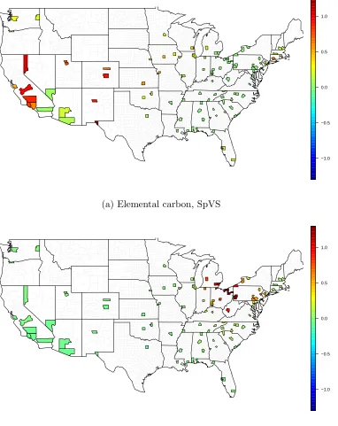
k and γks for the EVS model without effect mod-ification ((a)-(b)), the VS with effect modifiers model ((c)-(d)), and the unsmoothed VS with effect modifiers model when there is no shared mean for the ξk coefficients ((e)-(f)). . . 41 Figure 3.4 Estimated RR for elemental carbon by county for EVS model (top) and
Effect modifier VS model (bottom) . . . 42 Figure 3.5 Posterior mean and standard deviation ofξ parameters in the effect
Figure 4.1 One realization from the indicator model and from our copula prior on a 100×100 grid. In both,αk= 0.5,ωk = 0.2, andπk = 0.5. The continuous part of the two-indicator model are drawn from a GPex(0.5, 0.2, 10) model, such that spatial correlation at neighboring sites is about 0.9. The binary part is γk(s) ∼ Bernoulli{Φ[zk(s)]}, where zk(s) are GPex(0, 1, 10) and drawn independently from the continuous part. The latent copula
θ∼GPex(0,0,10) from the same seed as the continuous part of the two-process model, to give similar pictures. This example is the copula model
with C=∞ to give exact zeros. . . 48
Figure 4.2 A comparison of the joint density of βk(s) and βk(s0) under an indicator model (a) and our copula model (b). In (a), βk(s) = γk(s)Bk(s), where γk(s)⊥γk(s0), andBk(s),Bk(s) are multivariate normal with correlation ρ. In (b), our copula model whereγk(s),βk(s0) joined by Gaussian copula with correlation ρ. For both plots, the marginal density is the mixture in (4.2), with π = 0.8,α= 0.5,ω = 0.5, and the correlation isρ= 0.9. . . 49
Figure 4.3 Estimated county-specific relative risk for an IQR increase in elemental carbon from exchangeable VS model. . . 56
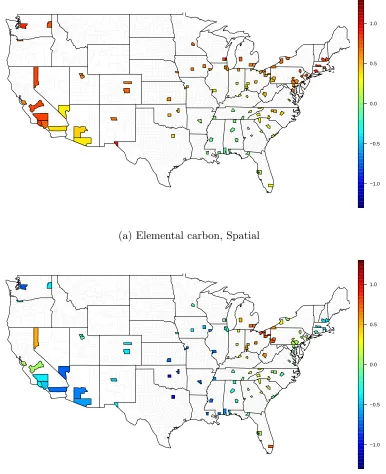
Figure 4.4 Estimated county-specific relative risk for an IQR increase in elemental carbon (a) and organic carbon (b) from the SpVS model. . . 62
Figure 4.5 Estimated county-specific relative risk for an IQR increase in elemental carbon (a) and organic carbon (b) from the Spatial model. . . 63
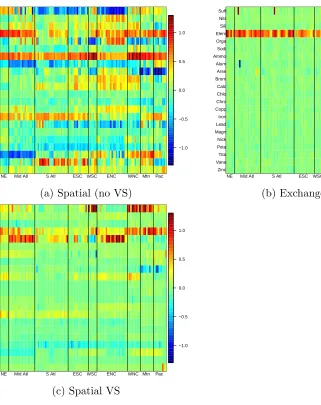
Figure 4.6 Matrix of all estimated coefficients (in RR per IQR increase) for each of the six models in Table 1. Each row includes coefficients for the labeled pollutant; each column indicates one county. The counties are grouped according to the 8 EPA subregions. The purpose of this plot is to highlight differences in local estimates for each of the models. . . 64
Figure B.1 Proportion of population which is Hispanic. . . 73
Figure B.2 Proportion of population which is Black. . . 74
Figure B.3 Proportion of adults over age 65 in poverty. . . 74
Figure B.4 Proportion of population commuting by public transit. . . 75
Figure B.5 Proportion of population living in an urban center. . . 75
Figure B.6 Median year built for all occupied housing. . . 76
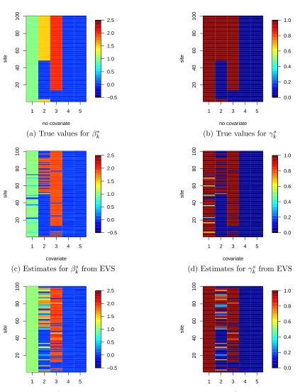
Figure B.7 True values for βs k and γsk from a simulated example and the resulting estimated parameters from an EVS model and a VS model with effect modifiers. . . 78
Figure D.1 Percent relative risk increase for one IQR increase of Sulfate from the SpVS model with 22 pollutants. . . 81
Figure D.2 Percent relative risk increase for one IQR increase of Nitrate from the SpVS model with 22 pollutants. . . 82
Figure D.3 Percent relative risk increase for one IQR increase of Silicon from the SpVS model with 22 pollutants. . . 82
Figure D.5 Percent relative risk increase for one IQR increase of Organic carbon from the SpVS model with 22 pollutants. . . 83 Figure D.6 Percent relative risk increase for one IQR increase of Sodium from the
SpVS model with 22 pollutants. . . 84 Figure D.7 Percent relative risk increase for one IQR increase of Ammonium from
the SpVS model with 22 pollutants. . . 84 Figure D.8 Percent relative risk increase for one IQR increase of Aluminum from the
SpVS model with 22 pollutants. . . 85 Figure D.9 Percent relative risk increase for one IQR increase of Arsenic from the
SpVS model with 22 pollutants. . . 85 Figure D.10 Percent relative risk increase for one IQR increase of Bromine from the
SpVS model with 22 pollutants. . . 86 Figure D.11 Percent relative risk increase for one IQR increase of Calcium from the
SpVS model with 22 pollutants. . . 86 Figure D.12 Percent relative risk increase for one IQR increase of Chlorine from the
SpVS model with 22 pollutants. . . 87 Figure D.13 Percent relative risk increase for one IQR increase of Chromium from the
SpVS model with 22 pollutants. . . 87 Figure D.14 Percent relative risk increase for one IQR increase of Copper from the
SpVS model with 22 pollutants. . . 88 Figure D.15 Percent relative risk increase for one IQR increase of Iron from the SpVS
model with 22 pollutants. . . 88 Figure D.16 Percent relative risk increase for one IQR increase of Lead from the SpVS
model with 22 pollutants. . . 89 Figure D.17 Percent relative risk increase for one IQR increase of Magnesium from the
SpVS model with 22 pollutants. . . 89 Figure D.18 Percent relative risk increase for one IQR increase of Nickel from the SpVS
model with 22 pollutants. . . 90 Figure D.19 Percent relative risk increase for one IQR increase of Potassium from the
SpVS model with 22 pollutants. . . 90 Figure D.20 Percent relative risk increase for one IQR increase of Titanium from the
SpVS model with 22 pollutants. . . 91 Figure D.21 Percent relative risk increase for one IQR increase of Vanadium from the
SpVS model with 22 pollutants. . . 91 Figure D.22 Percent relative risk increase for one IQR increase of Zinc from the SpVS
Chapter 1
Introduction
In this first chapter, we introduce background material and established methodology. We first introduce the idea of a copula, a mathematical structure for inducing correlation between ran-dom variables, which we use in Chapters 2 and 4. Secondly, we introduce Stochastic Search Variable Selection (SSVS), a common Bayesian computational approach to variable selection, which we extend in Chapters 3 and 4.
1.1
Copulas
A bivariate copula is a functionC(u, v) from [0,1]×[0,1] to [0,1] that has certain mathematical properties (see Nelsen (1999)). First discussed by Sklar (Sklar, 1953), a copula binds or joins a joint distribution to its marginals in such a way that the dependence between variables is independent of the marginal distributions. For one of our most familiar joint distributions, the multivariate normal distribution, the joint distribution fully characterizes the marginal distribu-tions of each random variable, as well as their dependence. For normal marginal distribudistribu-tions, however, the usual multivariate distribution is not the only valid joint distribution. Conversely, the dependence structure implied by the multivariate normal distribution can also be applied to random variables with non-normal marginals to create a valid joint density. However, given the marginal distributions and dependence structure implied by the joint distribution of the usual multivariate normal, there is a unique copula (known as the Gaussian copula) that binds this joint distribution to its marginals. These results are concisely reported in Sklar’s Theorem for bivariate densities:
Theorem 1. Sklar’s Theorem Given random variables X,Y, with (marginal) distribution functions F(x) =P(X < x) and G(y) = P(Y < y), and joint distribution H(x, y) = P(X <
x, Y < x), there exists a copula, CXY such that H(x, y) = CXY[F(x), G(y)]. If F and G
H(x, y) =C(F(x), G(y)) is a valid joint distribution.
This result readily extends ton-dimensional multivariate distributions and copulas (Nelsen, 1999). As another example, consider one of the simplest copulas, the product copula. Clearly Π(u, v) =uvdefines a valid joint distribution; for variablesXandY with marginal cdfsF andG, the implied cdf is that for independent random variables,H(x, y) = Π(F(x), G(y)) =F(x)G(y). We can write the Gaussian copula described above as CΣ(u, v) = ΦΣ(Φ−1(u),Φ−1(v)), where
ΦΣ is the multivariate normal cdf with covariance matrix Σ and CΣ refers to the resulting
Gaussian copula.
We can see further the usefulness of copulas by considering the following theorem:
Theorem 2: Invariance to transformation LetX,Y be continuous random variables with marginal distribution functionsF1, G1 and copulaCXY binding them to their joint distribution
H1(x, y). Let α, β be strictly increasing functions on Range(X) and Range(Y) respectively.
Then CXY =Cα(X)β(Y).
To prove, let F2(x) = P(α(X) < x) = P(X < α−1(x)) =F1(α−1(x)), and similarly G2(y)
denote the cdfs of the random variables X∗ = α(X), Y∗ =β(Y). Then, the joint distribution of α(X), β(Y) is
H2(x, y) = Cα(X),β(Y)(F2(x), G2(x)) =P(X < α−1(x), Y < β−1(y))
= CXY(F1(α−1(x)), G1(β1(y))) =CXY(F2(x), G2(y)).
That is, given a set of marginal and joint distributionsF, G, H and their corresponding copula
CXY, we can easily find the joint distribution of α(X), β(Y). The same copula that binds the marginal of X and Y to their joint distributionH1 can be used to bind the marginals of α(X)
and β(Y) to their joint distribution, H2. This result also extends to the n-dimensional case
(Nelsen, 1999). This reiterates the point that the dependence structure of the model is specified independently of the marginal distributions.
1.2
Comparison of the Gaussian and t-copulas
The Gaussian copula is often criticized because of the lack of dependence in the tails of the distribution. The t-copula, which is generated from the multivariate-t distribution, is another useful copula, which shares the elliptical properties of the Gaussian copula, but allows for greater dependence in the tails. First, the t-copula is defined as
Cν,TΣ(u1, . . . , un) =Tν,Σ tν−1(u1), . . . , t−ν1(un)
where t−ν1 is the inverse cdf of a univariate central t-distribution with ν degrees of freedom, and Tν,Σ is the multivariate-t cdf. The d-dimensional multivariate-t density with ν degrees of
freedom, center µ, and covariance Σ), is
Γ ν+2d Γ ν2 p(πν)d|Σ|
1 +(x−µ)
TΣ−1(x−µ)
ν
−ν+2d
as described by Demarta and McNeil (2005), and we write x∼td(ν,µ,Σ).
Note that the multivariate-t can be represented as a multivariate normal mixture, such that x=d µ+√Wz, where z is independent of W, z∼N(0,Σ) and 1/W ∼gamma(ν/2, ν/2). This fact is simply an extension of the univariate case, a result which is familiar from inducing a t distribution in Gibbs’ sampling through a hyperprior on the variance. This fact will also make simulation and MCMC sampling from a t-copula computationally convenient. Note that as the copula is invariant to any monotone transformation (see Theorem 2 above), utilizing a correlation matrix as Σ in the t-copula will be sufficient.
The differences between the Gaussian copula and t-copula can be dramatically demon-strated using joint quantile exceedance probabilities, that is, the probability that multiple ex-treme events will happen simultaneously. The joint exceedance probabilities for the t-copula are greater than those for the Gaussian copula. As one would expect, the ratio of the t to Gaussian exceedance probabilities grows as degrees of freedom decreases (t becomes less like Normal), but also grows with increasing correlation and dimension of the copula. When extreme values are of interest, misspecification of the copula can become extremely important, for instance in hydrology and finance. As an extreme example, Demarta and McNeil (2005) describe finding the probability that 5 correlated stocks will drop to the lowest 1% of their marginal distribu-tions on the same day. When the joint distribution is generated using at4 copula, and bivariate
correlations of 50%, this event will occur approximately every 7 years. However, a Gaussian copula fit to these data suggest it is a 1 in 50 year event.
and asymptotic conditional probability defined as
lim
q→1P(X2> F
−1
2 (q)|X1 > F1−1(q)) =λu
for the upper coefficient, and a similar definition for λl, the lower coefficient. For ellipti-cally symmetric copulas such as the Gaussian and t-copulas, both coefficients are the same, and we will refer simply to λ. For the Gaussian copula, λ = 0, and for the t-copula, λ = 2tν+1
−p
(ν+ 1)p(1−ρ)/p(1 +ρ)
, which will always be positive (Demarta and McNeil, 2005), again indicating stronger tail dependence for the t copula. We will use both thetcopula and Gaussian copula in Chapter 2, to implement a spatially correlated bridge distribution for random effects in logistic regression.
1.3
Stochastic Search Variable Selection
When faced with a large number of potential predictors, variable selection can be a powerful tool, both statistically and scientifically. By reducing the number of variables in the model, standard error of estimates and prediction intervals decrease. From a scientific perspective, variable selection can help identify which variables are most important, or at least most strongly associated with the outcome. From a Bayesian perspective, optimal model selection would involve fitting all possible models, and comparing Bayes factors. As the number of potential models with p predictors is 2p, this quickly becomes intractable. Stochastic Search Variable Selection (George and McCulloch, 1993; George and McCulloch, 1997) has become a vastly popular tool for selecting among a large set of potential predictors, as the highest probability models are sampled using MCMC methods. Consider a linear model relating a responseyt for
t= 1, . . . , T and covariatesxkt fork= 1, . . . , ppredictors,
yt = x1tβ1+. . .+xptβp+εt,
where εt are Gaussian errors. Let βk be the coefficient on predictork, and βk =γkBk where,
γk is a binary random variable, and Bk continuous. This implies the kth covariate, xk, is “in” if γk = 1, and “out” if γk = 0. The stochastic search model easily allows for calculating the posterior mean of γk, i.e., the posterior probability that the kth covariate is in the model, as well as the joint posterior probability of any subset of γ1, . . . , γp, thus allowing for an easy way to compare models without having to compute Bayes factors for every possible subset. SSVS is implemented within Gibbs sampling whereγk ∼Bernoulli(π) andBk ∼N(0, ω2), whereω2 is some large variance. For the linear model with Gaussian errors the model is fully conjugate.
−2 −1 0 1 2
0
1
2
3
4
5
6
beta
Figure 1.1: The spike-and-slab prior used in Stochastic Search Variable Selection, withπ= 0.1,
ω= 1, and C= 150.
mixture with probabilityπ,
βk ∼N
(
N(0, ω2) with probabilityπ
N(0, ω2/C) with probability1−π (1.1)
where C is a large number controlling the ratio of variance when βk is included in the model and when it is excluded. When C = ∞, this reduces to the binary-product case above. This prior distribution is shown in Figure 1.1. This prior reflects the belief that many covariates will have no appreciable effect on the response (βk ≈0), and some will have a large effect. In this thesis we consider a hierarchical Bayesian model in which we are interested in selecting amongstppredictors atnsites. In Chapter 3, we consider modeling the inclusion probabilityπ
Chapter 2
Bridging Conditional and Marginal
Inference for Spatially-Referenced
Binary Data
2.1
Introduction
Spatially-referenced binary data abounds in the fields of epidemiology, public health, geography and image processing, among others. For valid inference on model parameters, it is important to account for correlation indexed by proximity due to the unmeasured spatial factors. While linear mixed models easily allow the incorporation of correlated random effects (REs), logistic regression and other generalized linear mixed models (GLMM) suffer an interpretation problem (i.e. a mismatch between conditional and marginal distributional shapes) due to the nonlinearity of the mean function. Because of this, researchers usually choose between a marginal model for ‘population-averaged’ inference, or a conditional model for ‘subject-specific’ inference for the regression parameters, primarily motivated by inferential objectives. The regression effects can be different at each level due to subject or site level variability, particularly when this variability is large, highlighting the importance of proper interpretation. While model goodness of fit is certainly an important consideration in choosing a random effects distribution, interpretability is essential. In this chapter, we propose a model for spatial binary data that preserves the log odds interpretation of covariate effects both conditional on and marginal over REs.
gender on the periodontal decay status of each tooth, which requires properly accounting for clustering within subjects and spatial dependence between teeth. Earlier studies (Reich et al., 2007; Reich and Bandyopadhyay, 2010) have shown that periodontal disease markers might be spatially-associated, as a diseased (or decayed) tooth (or sites within a tooth) might be influ-encing the periodontal health status of a set of neighboring sites or teeth. Therefore, in addition to independent subject-specific RE, we include spatially correlated RE for each tooth nested within subjects.
The usual Gaussian RE logistic regression model for spatially-referenced binary data may not be well-suited here where the regression coefficients are only interpretable conditioned on the spatial REs, and thus in terms of replication at the same location for a given subject. In a more traditional disease mapping setting (with many subjects observed at each spatial location) when researchers are possibly interested in a site-specific interpretation (conditional on county of residence), these conditional parameters have meaning. However, for our data, an interpretation conditioned on tooth REs is purely hypothetical as we cannot take another replicate of the same tooth for the same subject. A similar objection arises for interpreting subject-level covariate effects such as gender, age, etc conditional on the subject. However, coefficients for certain ‘tooth-level’ measures, such as an indicator of molar, could plausibly be interpreted conditional on a subject RE. Hence, we desire a model with interpretable parameters both conditioned on, and marginal over subject and tooth RE.
et al., 2009). In this Markovian model, the coefficients have a log-odds interpretation condi-tioned on a pre-defined neighbor set. Though the full conditional distributions are intuitive, they lead to a complicated joint spatial distribution (Varin et al., 2011), and the marginal ef-fects of covariates are not readily available. Further, it is unclear how to extend this model to geostatistical data defined continuously on a given spatial domain.
Wang and Louis (2003, 2004) made headway in solving the conditional-marginal dilemma for random-intercept logistic regression by proposing a new distribution (for the random in-tercepts), aptly named the ‘bridge distribution’. The marginal and conditional mean have the same form, and the marginal regression coefficients are proportional to the conditional regres-sion coefficients. It falls under the general definition of marginalized models (Griswold and Zeger, 2004), amenable to a likelihood-based analysis through standard software, but is unique in that it retains the log-odds ratio interpretation both conditionally and marginally.
Motivated by the periodontal data, here we exploit the richness of the Wang and Louis model to study marginal/population-level covariate effects for spatially distributed binary data. This strength becomes further important in richer hierarchical models, such as the nested subject-and site-specific REs we use for the periodontal data, where the coefficients can easily be interpreted at whichever level of the hierarchy is desired. Extension to this setup for bivariate binary responses (Li et al., 2011) and a binary and continuous response (Lin et al., 2010) have been demonstrated. Here we provide a full exploration of a multivariate bridge distribution and its application in a nested REs setting. The spatial bridge distribution is derived using a Gaussian copula, and extensions to a more general t-copula are also presented. Although our model development is currently tailored towards the specific structure of dental data, it can be applied to more conventional spatial settings with a single observation at each location, or with multiple subjects observed at the same site. Our model that incorporates both subject-and site-specific REs can simultaneously estimate covariate effects conditioned on both the REs, marginally over subject- and site-specific REs. Identification of high-risk areas through estimation of REs is possible within our unified framework, often precluded in a marginal model. Our hierarchical Bayesian scheme has computational complexity equivalent to the usual Gaussian RE model, and can easily be implemented in standard software such as OpenBUGS.
2.2
The spatial bridge distribution
For notational convenience, we specify the model assuming all n subjects have observations at the same m spatial locations s1, . . . , sm. Extending to more complex designs is straight-forward using our Bayesian hierarchical model. In particular, we do not require replication at each spatial location or a balanced design across subjects. The binary response Yij for subject i at site sj is modeled as Yij|εij ∼ Bernoulli(πij), with logit(πij|Xij, εij) = XijβS+
εij, where πij is the Bernoulli success probability, Xij is the design matrix of covariates, βS is the regression vector (the superscript ‘S’ denotes site-specific conditional parametrization of regressors), and εi = (εi1, . . . , εim)0 is the vector of spatial REs for subject i, which are independent and identically distributed.
In addition to the Bernoulli probability conditional on the REs, we are also interested in the Bernoulli probability marginal over the REs,πP
ij =
R
πijg(εij)dεij.For most RE densitiesg(εij), including Gaussian, this marginal probability is unknown and must be computed numerically. In the spirit of Wang and Louis (2003), to preserve the logistic shape both conditionally and marginally we allow εij to follow the bridge density given by
g(ε;φ) = 1
2π
sin(φπ)
cosh(φε) + cos(φπ), (2.1)
where cosh(x) = 12(ex+e−x). We denote this as ε∼ bridge(φ), where 0 < φ <1 controls the variance and shape of the density. The bridge density is mean 0 and varianceσb2 = π32(φ−2−1), and like the normal distribution is symmetric and bell-shaped, though it has heavier tails. We assume φto be common for all observations to assure exchangeability across the spatial units. With such a bridge structure forε, the marginal regression model is
logit(πPij) =XijβP,
where βP is the marginal (population-level) parameter vector and is related to βS by βP =
φβS = q 1
1+3
π2σ
2
b
βS. This is a development over the marginal interpretation under the Gaussian
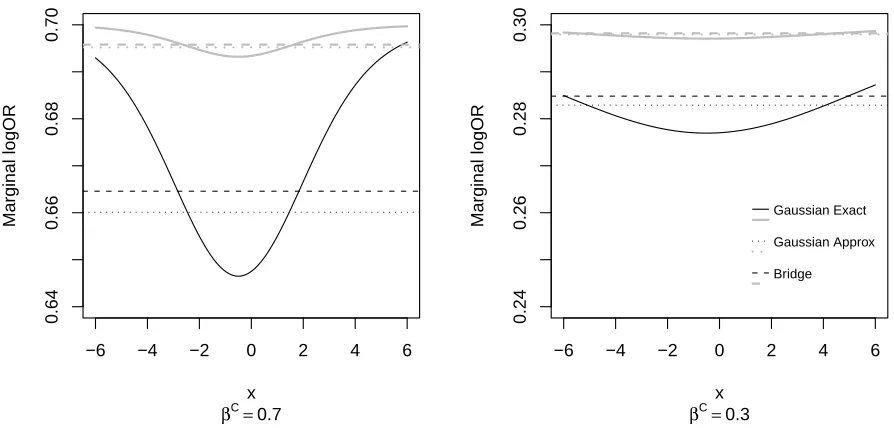
REs model. The exact marginal log odds for Gaussian REs is nonlinear in X, with nonlinearity increasing with REs variance and the strength of conditional association,βS. Johnson and Kotz (1970) give the approximation logit(πP
ij) ≈ XijβP where βP = q 1
1+(1615)2 3
π2σ
2β
S. Figure 2.1
shows the relationship between the exact and approximate marginal log odds ratio (calculated numerically as a function of X) for a model with a single predictor. For comparison, the marginal log odds ratio that would result from assuming a bridge random effects distribution with the same variance is also shown. We observe notable differences between these curves, and that as
−6 −4 −2 0 2 4 6
0.64
0.66
0.68
0.70
βC=
0.7 x
Marginal logOR
−6 −4 −2 0 2 4 6
0.24
0.26
0.28
0.30
βC=
0.3 x
Marginal logOR Gaussian Exact
Gaussian Approx
Bridge
Figure 2.1: Marginal log odds ratio for unit increase from X to X+1, when the random effects follow a Gaussian or bridge distribution. In both graphs, gray lines have random effects standard deviationσ = 0.2, and black lines have random effects standard deviationσ = 0.6
To extend the bridge model from the exchangeable to the spatial setting, we make use of a copula (Sklar, 1953, 1973; Nelsen, 1999) to capture spatial correlation while preserving the marginal bridge distribution at each location. Let θi be a latent Gaussian process for subjecti with zero mean, unit variance and spatial correlation function cor[θ(s), θ(s0)] =ρ(ks−s0k). One example of a correlation function is the the exponential correlation defined by ρ(ks−s0k) =
e−ks−s0k/r, wherer >0 controls the spatial range of the latent process. Marginal bridge distri-butions are forced via the probability integral transformation
εij =G−φ1{Φ [θi(sj)]}, (2.2)
where Φ is the cumulative distribution function (c.d.f) of N(0,1) andG−φ1 is the inverse c.d.f of the univariate bridge density available in a closed form (Li et al., 2011) given by G−φ1(y) =
1
φlog
h
sin(φπy) sin(φπ(1−y))
i
, for 0< y <1. We fix the variance ofθi(s) at one for alls, because only the correlation structure is important in the copula specification. If θi(s) has a non-unit variance
Utilizing a Gaussian copula, the joint cumulative distribution of εi, is given by
H(εi1, . . . , εim) = ΦΣr
Φ−1[Gφ(εi1)], . . . ,Φ−1[Gφ(εim)] ,
where Σr is the m×m covariance matrix ofθi = (θi1, . . . , θim). We denote this model as εi ∼ bridge(φ,Σr). Though motivated here from a geostatistical perspective, any valid correlation matrix, including the correlation implied by a conditionally autoregressive (CAR) model for areal data (Banerjee et al., 2004) could be used in place of Σr. Under this copula model, the random effects εi are non-Gaussian, but maintain the Markovian dependency structure of the CAR model.
Although the Gaussian copula is an intuitive way to induce spatial correlation, it may not capture tail dependence (Demarta and McNeil, 2005). A logical alternative is the t-copula, which can be easily implemented within the Bayesian framework. The t-copula assumes that
θi iid
∼tν(0,Σr), wheretν is the multivariatetdistribution with location 0, scale matrix Σrandν degrees of freedom. We can either fixν, or assign it an additional hyperprior. Similarly as above,
εij = G−φ1[Tν(θij)], where Tν is the c.d.f of a mean 0 univariate t distribution with ν degrees of freedom. Visual comparison (Figure 2.2) of the bivariate bridge densities for the Gaussian andt-copula at two levels of correlation reveal differences particularly in the tails. More flexible copulas such as the non-parametric copula as in Fuentes et al. (2013) can be used, but with the limited information available in our binary response, the parametric t-copula is likely flexible enough to capture important dependence.
To quantify the effect on the correlation function due to the probability integral transfor-mation, Figure 2.3 plots the correllogram assuming exponential and Matern spatial correlation functions, and Gaussian and t copulas. We find that for both correlation functions and copulas, the correlation function of the copula models has the same general shape as correlation function of the latent Gaussian process, but the magnitude of correlation is slightly lower. This may be useful when specifying informative priors for the spatial correlation parameters.
Spatial prediction of the random effect εi(s0) at prediction location s0 follows from
stan-dard Bayesian Kriging methods. Using the Gaussian copula, we sample θi(s0)|θi using prop-erties of the conditional distribution of a multivariate normal, and then transform to εi(s0) =
G−φ1{Φ [θi(s0)]}. For the t-copula, the same approach can be used after exploiting the
hier-archical representation of the multivariate t. If we assume that θi|τi ∼ N(0, τi2Σr), where
τi−2 ∼ gamma(ν/2, ν/2), then θi follows a multivariate tν(0,Σr) marginally over τi. Spatial interpolation can be done conditional onτi as with the Gaussian copula.
which there are REs for both subjects and sites within subjects, given as:
logit{P(Yij = 1|Xij, γi, εij)}=XijβT +γi+εij, (2.3)
whereγi are independent subject-specific REs andεij are tooth-level REs. A slight complication arises with multiple REs because the bridge distribution is not additive or a scale family. As suggested by Wang and Louis (2003), we assume γi = γi∗/φ2, and that γi∗
iid
∼ bridge(φ1) and εi ∼bridge(φ2,Σr). In this case we are interested in estimating the log odds at each level of the hierarchy. We let the ‘site-within-subject’ level coefficient βT denote the conditional log odds ratio, using ‘T’ to signify a ‘tooth’-level interpretation. After integrating over the tooth REs εi, we have logit{P(Yij = 1|Xij, γi∗)} = XijβS +γi∗, and the coefficient βS = φ2βT
represents the ‘subject’-level interpretation, in that it can only be interpreted conditional on the subject REs γi. Finally, βP is the ‘population’-level, or completely marginal coefficient, with logit{P(Yij = 1|Xij)}=XijβP. The population level log odds ratios are defined by βP =
φ1φ2βT. Also, we denote the total subject level standard deviationσ1= sd(γi), and the standard deviation of the bridge REs controlled by φ1, σ1∗ = sd(γ∗i). Further, σ2=sd(εij) represents the standard deviation of the site-specific REs, controlled byφ2. A nested RE structure is also easily
implemented in other studies where perhapsγi are spatially correlated (e.g. county effects) and
εij are independent (e.g. subjects within a county).
2.3
MCMC implementation
We implement the model using R (R Development Core Team, 2010) (Web Appendix A) for the simulation study, andOpenBUGS(Web Appendix B) for the dental data example.OpenBUGS
coding for this model is a very simple extension from the usual Gaussian model, by treating
εij as a transformation of a latent Gaussian variable θij. Implementation of the model with thet-copula requires thetν cdf, which, unlike the Gaussian cdf, is not an available function in
OpenBUGS. However, this cdf exists in closed form forν= 2, and so for the dental analysis with
t-copula, we hold ν fixed at 2, rather than include a prior for ν. We ran 10,000 samples with 3000 burn-in for the simulated data, and visually monitored convergence by starting multiple chains from diverse starting values for a selection of datasets. For the dental data analysis, we used 25,000 iterations with 5000 burn-in.
2.4
Simulation Study
estimates to misspecification of the RE distribution and identify the situations that lead to the most sensitivity. Earlier work has already considered the effect of misspecification in logistic regression models with independent, identically distributed random intercepts. Neuhaus et al. (1992) show that for a true RE distributionG, and an assumed RE distributionF, the maximum likelihood estimates under F minimize Kullback-Leibler divergence of the marginal models implied under G and F. Asymptotically and in simulation, they show that for any F and G
the bias of the MLE for the conditional coefficient βS are expected to be small, but that bias forσ may be large. It is unclear whether these results extend to a correlated intercepts setting and a Bayesian model. Furthermore, because the marginal interpretation depends directly on variance, and Neuhaus et al. (1992) show the variance is heavily biased, it is unclear how this will affect bias in the marginal estimates.
In this study, we consider n = 100 subjects, each with observations at m = 14 spatially correlated sites to mimic the structure of our dental data where each subject has 28 teeth. The fourteen spatial locations are equally spaced along a line of length one, representing the structure of one jaw. The data are generated from the nested REs model in (2.3). We consider
p = 4 covariates, two of which are ‘subject level’ and two of which are ‘site level’. The sub-ject level covariates X1 and X3 take the same value for all sites for subject i, while X2 and
X4 (the site level ones) vary across sites and subjects. All four covariates were drawn
inde-pendently from standard normal distributions. The values for the conditional coefficients are
βT = (0.5,0.5,1,1)T. Thus, we can simultaneously compare the sensitivity to REs distribution for subject- and site-level covariates, and large and small coefficients. The correlation matrix of the site-specific effects is taken to be exponential with spatial ranger= 0.1 or 0.4. The standard deviation of the subject REs, σ1∗, is fixed at 1, while the standard deviation of the site-level REs is chosen to be either σ2 = 1 or 3. The total marginal shrinkage, φ1φ2, is either 0.77 or
0.45. We consider four design settings for data generation:
Design 1: Low Variance and low spatial correlation, i.e., σ2 = 1, r= 0.1
Design 2: Low Variance and high spatial correlation, i.e., σ2= 1, r= 0.4
Design 3: High Variance and low spatial correlation, i.e.,σ2 = 3, r = 0.1
Design 4: High Variance and high spatial correlation, i.e., σ2 = 3, r= 0.4
At each design setting, we generate 100 datasets assuming the true REs distribution is either Gaussian or bridge. When generating the data from a Gaussian distribution, we directly generateγi∼N(0, σ12). For each dataset, we fit the logistic model with Gaussian REs and bridge
bias and root mean square error (√MSE), each calculated with respect to the posterior mean forβT,βS andβP. For the marginal βP in the Gaussian REs models, the ‘true’ value will be the approximation as in Johnson and Kotz (1970) (described in Section 2), applied twice. The model is parameterized in terms of the precision of the REs distributions, so the same priors can be used for either Gaussian or bridge REs. We assume the priors 1/σ∗12∼gamma(1,0.25) and 1/σ22 ∼gamma(1,0.25). We use a normal prior with variance 100 for β, where the coefficients are independent a priori.
Tables 2.1, 2.2 and 2.3 present the effect of misspecification on marginal inference. The relative percent bias in all models ranges from 0 to ±10%. As expected, when the true RE distribution is Gaussian, the Gaussian fit has slightly smaller bias and√MSE than the bridge fit and vice versa. The relative √MSEs in Table 2.3 are generally closer to one in the first case where Gaussian model is true and the bridge model is misspecified, compared to the other case where the bridge model is true and the Gaussian model is misspecified. It may be that by including shape parameter φ the bridge distribution is more robust than the Gaussian model. The largest difference we observe is forβ1 when the bridge model is true. This is a subject-level
covariate with a small coefficient; the √MSE is 10-25% greater for the misspecified Gaussian model than the bridge depending on the covariance parameters. The bridge model also compares favorable to the GEE approach. Because the difference in shape of the bridge and Gaussian distribution is more pronounced as variance decreases, we expect larger differences between models for σ2 = 1 and this is generally the case. Frequentist coverage probability (not shown)
for all coefficient estimates is close to the nominal 95%. Across all model fits, we find that the
√
MSE for the coefficients on subject specific covariatesX1 and X3 is nearly twice that of the
site specific covariatesX2 and X4. The size of the coefficient does not appear to have an effect.
0 1 2 3 4 5
−1.0 −0.5 0.0 0.5 1.0
−1.0 −0.5 0.0 0.5 1.0 0 1 2 3 4 5
−1.0 −0.5 0.0 0.5 1.0
−1.0 −0.5 0.0 0.5 1.0 (a) (b) 0 2 4 6 8
−1.0 −0.5 0.0 0.5 1.0
−1.0 −0.5 0.0 0.5 1.0 0 2 4 6 8
−1.0 −0.5 0.0 0.5 1.0
−1.0 −0.5 0.0 0.5 1.0 (c) (d)
Figure 2.2: Bivariate density for (a) Bridge with Gaussian copula andρ= 0.3 (b) Bridge with
t-copula,ρ= 0.3 andν= 2 degrees of freedom (c) Bridge with Gaussian copula andρ= 0.8 and (d) Bridge witht-copula,ρ= 0.8, andν = 2. In all graphs,φ=.95, for a standard deviation of
0.0 0.1 0.2 0.3 0.4 0.5
0.0
0.2
0.4
0.6
0.8
1.0
Distance
Correlation
Gaussian
Bridge, Gauss cop Bridge, t cop
(a)
0.0 0.1 0.2 0.3 0.4 0.5
0.0
0.2
0.4
0.6
0.8
1.0
Distance
Correlation
Gaussian
Bridge, Gauss cop Bridge, t cop
(b)
Figure 2.3: Comparison of correlation by distance for bivariate Gaussian distribution and bridge distribution with φ = 0.95 using a Gaussian and t2 copula. The plots compare (a)
Table 2.1: Relative percent bias of population-level coefficients when the underlying true model is Gaussian and bridge. ‘G’ indicates fit of the Gaussian model, ‘B’ indicates the bridge model fit, and ‘GEE’ indicates the GEE fit. Results which show a significant difference from the bridge model are indicated with ‘*’.
Gaussian distribution is ‘true’
σ2 = 1 σ2= 3
r = 0.10 r = 0.40 r= 0.10 r = 0.40
G B GEE G B GEE G B GEE G B GEE
βP
1 2.13* -2.92 0.43* -3.57* 1.45 -0.34* 1.41* 5.22 2.18 1.47* 4.60 1.35
βP2 -3.27* -6.19 -5.45 -3.56* -0.48 -3.19 -6.45* -3.02 -5.82 -4.83* -2.07 -5.37
βP3 2.27* -1.34 1.12* -1.96* 1.97 0.99* -3.10* 1.46 -0.22* -1.25* 2.17 0.72*
βP4 0.67 -2.03 -0.60* -2.28* 0.54 -0.94* -1.77* 1.54 -1.12* -2.86* -0.03 -2.65
Bridge distribution is ‘true’
σ2 = 1 σ2= 3
r = 0.10 r = 0.40 r= 0.10 r = 0.40
G B GEE G B GEE G B GEE G B GEE
βP
1 4.32 2.80 3.46 3.82 1.95 2.94 8.80* 5.62 6.44 6.15 4.86 4.02
βP2 1.10* -2.74 -0.58 2.91* 1.51 0.92 0.60* -1.54 -1.67 0.81* -1.48 -2.05
βP3 3.37 3.77 2.68 3.43 2.56 2.63 4.31* 2.02 2.53 5.84* 4.25 4.40
βP
Table 2.2: √MSE×100 when the underlying true model is Gaussian and bridge. ‘G’ indicates fit of the Gaussian model, ‘B’ indicates the bridge model fit, and ‘GEE’ indicates the GEE fit. Results which show a significant difference from the bridge model are indicated with ‘*’.
Gaussian distribution is ‘true’
σ2 = 1 σ2 = 3
r = 0.10 r = 0.40 r = 0.10 r = 0.40
G B GEE G B GEE G B GEE G B GEE
β1P 11.68 11.70 11.86 13.66 13.70 13.68 11.50 11.23 11.26 13.75 13.61 13.52
β2P 6.34 6.46 6.51 5.89 5.89 6.12 6.82 6.72 6.82 6.30 6.24 6.54
β3P 11.13 11.18 11.35 12.08 12.31 12.22 10.35 10.63 10.40 12.48 12.95 12.70
β4P 6.40 6.68 6.45 6.32 6.57 6.64 6.59 6.49 6.58 6.48 6.52 6.65
Bridge distribution is ‘true’
σ2 = 1 σ2 = 3
r = 0.10 r = 0.40 r = 0.10 r = 0.40
G B GEE G B GEE G B GEE G B GEE
β1P 11.05* 8.85 11.00* 12.91* 11.53 12.53 11.08* 10.01 10.93* 13.41* 12.11 13.13
β2P 6.60 6.26 6.58 6.16 5.99 6.22 6.60 6.42 6.37 6.29 6.20 6.27
β3P 10.55 11.05 10.57 11.76 11.87 11.92* 10.61 9.92 10.39* 13.19 13.60 13.35*
Table 2.3: The relative MSE of the Gaussian and bridge models.
Gaussian is true Bridge is true
σ2 = 1 σ2 = 3 σ2= 1 σ2 = 3
r= 0.10 r= 0.40 r = 0.10 r = 0.40 r= 0.10 r = 0.40 r= 0.10 r= 0.40
β1P 1.00 1.00 1.02 1.01 1.25 1.12 1.11 1.11
β2P 0.98 1.00 1.02 1.01 1.05 1.03 1.03 1.02
β3P 1.00 0.98 0.97 0.96 0.95 0.99 1.07 0.97
β4P 0.96 0.96 1.02 0.99 0.95 1.02 1.07 1.06
2.5
Dental Data example
The data consist of dental records for 260 Gullah-speaking African-Americans (Bandyopadhyay et al., 2010) in South Carolina. The location and clinical attachment level (CAL, in mm) were recorded by dental hygienists for each of the 28 adult teeth (excluding wisdom teeth), for each subject. As CAL is measured at multiple sites per tooth, we define a tooth as diseased if the mean CAL>3 mm, indicating moderate to severe periodontitis. The responseYij = 1 if tooth
j is missing or diseased for subjecti, and 0 otherwise. The subjects range in age from 26 to 87, are mostly female (75%), and are from an under-served population with generally poor health outcomes. Over 97% of the subjects have at least one missing or diseased tooth, and 55% have 10 or more missing or diseased teeth. For each subject, age, body mass index (BMI), smoking status, and HbA1c (a measure of blood-glucose level), are recorded, in addition to their dental health records. The objective of our analysis is to assess the oral health of this under-studied population, and identify the effects of these covariates on the (binary) oral health status, both at the population and subject specific level.
We fit the nested model in (2.3) assuming teeth in the upper and lower jaw are independent, and within each jaw, teeth are related by a first-order Markov model (i.e., an exponential covariance). A richer model would allow correlation between jaws where neighbors between jaws and within jaws have potentially different correlation. However, initial model fits suggest the correlation between jaws is negligible after accounting for subject REs, and treating each jaw independently reduces the size of our covariance matrix by half which drastically improves the speed of computation.
We fit this model assuming a Gaussian REs distribution, a bridge REs distribution with Gaussian copula, and a bridge REs distribution witht-copula. Here we fix the degrees of freedom
would allow ν to vary; however, because the t and Gaussian copulas are similar for large
ν, this will also allow for more contrast in the two approaches. For comparison, we also fit these models assuming only a subject RE by setting εij = 0. The prior for the coefficients
βkT iid∼ N(0,100), for k = 0, . . . , p, where β0T is the intercept term. The prior for the range parameter, r ∼ logNormal(−2,1), where the distance between teeth is standardized so the maximum distance is one unit. As in the simulation study, the prior for both standard deviations are 1/σk2 ∼ gamma(1,0.25). In addition to the Bayesian models, we also fit a GEE model (assuming independent subjects and an unstructured working correlation matrix), where the resulting estimates are only available at the (marginal) population level.
Results for the nested REs models appear in Tables 2.4 and 2.5. We compare these models using the Deviance Information Criterion (or DIC, Spiegelhalter et al. (2002)), popularly used in Bayesian inference, and defined as DIC = ¯D+pD, where ¯Dis the posterior mean of the deviance and pD is the effective number of parameters. Smaller values of DIC are preferred. A subject-only REs model appears to be inadequate here (DIC=6385 for bridge model) as expected, since we believe the implicit assumption of independent tooth effects is violated. The bridge model with both subject and tooth REs with a Gaussian copula has the lowest DIC of 4157. In addition to DIC, we calculated the Brier score, where we fit the model using 90% of the data randomly selected across teeth and subject, and estimate the posterior mean ˆπij for the remaining 10% (hold-out set). The Brier score (Brier, 1950) is then defined by N1 P
i,j(Yij −πˆij)2, whereN is the number of held out teeth (728). The Brier score ranges from 0 to 1, and smaller numbers are better. We further calculate the misclassification indices CV1 = N1−1
P
(i,s){Yijπˆij} and CV0 = N0−1P(i,s){(1−Yij)ˆπij}, where N1 = Pi,jYij, or the number of held out ones, and
N0 =Pi,j(1−Yij), or the number of held out zeros. We note that while the Brier score, CV1
and CV0are similar for all three models displayed in Table 2.4, the Brier score is also minimized
by the bridge model with Gaussian copula. To assess the statistical significance of these subtle differences in the Brier score, we repeated this test set validation ten times on a subset of 100 subjects and found the bridge model had smaller Brier score than the Gaussian model for seven of the ten splits, and a paired t-test on the difference in Brier had p-value 0.02. Also, the Brier score is higher for the subject only models (0.151 for Bridge, and 0.150 for Gaussian) than the spatial models in Table 2 (0.132 for the bridge and 0.134 for the Gaussian), again suggesting the nested REs models produce a better fit.
effects, we are left with a subject specific model with coefficients denoted by ‘S’ in Table 2.4. These coefficients are interpretable conditioned on the subject REs. For example, in the bridge model, we see the odds of a molar being missing or diseased aree2.15= 8.58 (95% credible set
[7.17, 10.18]) times higher than other teeth for the same subject. Age is also interpretable at both the subject and population level. For a given individual, the odds of diseased/missing teeth increases 90% with each standard deviation increase in age- about 10.9 years. At the population level, however, the odds of a diseased/missing teeth increase by 58%, the attenuation due to averaging over between subject variability characterized by σ1 in our model. It is important
to emphasize that the subject- and population-level coefficients for the Gaussian REs model displayed in Table 2.4 are approximations, while in the bridge model these represent the exact log odds ratio. The GEE estimates also represent an exact marginal log odds ratio, and remain comparable to the population level estimates for both the Bayesian models. The 95% intervals for the GEE analysis are generally wider than those from bridge model with Gaussian cop-ula, and unlike the Bayesian models the GEE analysis produces a (counterintuitive) significant protective effect of smoking on tooth loss.
Although various parameter estimates remain comparable across models, there are some notable differences. The nested REs model, the choice of RE distribution and copula has a large impact on the estimates. This is not surprising since different choices of REs/copula yield different scales, on which regression effects are estimated. For example, the population level estimate of the odds ratio corresponding to gender ise−0.39= 0.68 (0.49, 0.88) for the Gaussian
model, as compared to 0.57 (0.40, 0.76) for the bridge model with Gaussian copula. It should be noted that the impact is mainly on the magnitude of effect estimates, though the inference remains consistent across all three models, i.e., Age, Sex, HbA1c and the molar effect remain significant. Because of the relatively high degree of variation in the subject and tooth REs, there remain substantial differences in tooth-, subject-, and population-level interpretations of the coefficients. For example the estimated odds ratio for gender in the bridge model with Gaussian copula is eβT = 0.15 at the tooth level, 0.45 at the subject level, and 0.57 at the population level. This difference in the conditional and marginal interpretations highlights the importance of correctly choosing conditional or marginal inference. There are also differences in the covariance parameter estimates across models. The between tooth variability is estimated much lower for thet-copula model than the Gaussian copula model, resulting in a lesser degree of marginal shrinkage. For the subject-and-site models, note thatσ1=σ∗1/φ2 displayed in Table
2.5 is the total standard deviation of the subject REs γi, which depends on both φ1 and φ2.
This is much greater than the standard deviation found in the subject only model. The range parameter is about 0.15, regardless of copula, suggesting a correlation of 0.6 between adjacent teeth.
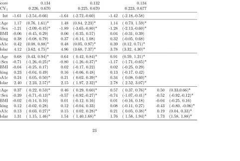
Table 2.4: Posterior parameter estimates and 95% credible intervals (C.I.) for tooth specific (T), subject specific (S) and population level (P) fixed-effects for the model with subject and tooth nested random effects. * indicates 95% C.I. that excludes 0. For the
t-copula, there areν = 2 degrees of freedom.
Gaussian Bridge: Gauss. copula Bridge: t-copula GEE
DIC 5283 4157 5490
pD 2578 1931 1692
Brier Score 0.134 0.132 0.134
CV0, CV1 0.226, 0.670 0.225, 0.670 0.223, 0.677
Int -1.61 (-2.54,-0.66) -1.64 (-2.72,-0.60) -1.42 (-2.18,-0.58) T:Age 1.17 (0.76, 1.61)* 1.48 (0.84, 2.23)* 1.14 ( 0.73, 1.59)*
T:Sex -1.21 (-2.09,-0.45)* -1.89 (-3.65,-0.80)* -1.28 (-2.13,-0.60)* T:BMI -0.06 (-0.45, 0.29) 0.06 (-0.35, 0.57) 0.04 (-0.31, 0.39) T:Smoking 0.38 (-0.08, 0.79) 0.37 (-0.14, 1.08) 0.32 (-0.05, 0.68) T:HbA1c 0.42 (0.08, 0.88)* 0.48 (0.05, 0.97)* 0.39 (0.12, 0.71)*
T:Molar 4.12 (3.62, 4.75)* 4.96 (3.68, 7.37)* 3.78 (3.32, 4.30)* S:Age 0.68 (0.43, 0.94)* 0.64 ( 0.42, 0.84)* 0.91 (0.59, 1.21)* S:Sex -0.71 (-1.26,-0.25)* -0.80 (-1.26,-0.37)* -1.17 (-1.71,-0.65)* S:BMI -0.04 (-0.25, 0.17) 0.02 (-0.17, 0.22) 0.02 (-0.25, 0.29) S:Smoking 0.23 (-0.04, 0.49) 0.16 (-0.06, 0.48) 0.13 (-0.17, 0.42) S:HbA1c 0.24 ( 0.05, 0.50)* 0.21 ( 0.02, 0.39)* 0.34 ( 0.08, 0.60)*
S:Molar 2.40 ( 2.23, 2.57)* 2.15 ( 1.97, 2.32)* 2.78 ( 2.52, 3.07)*
P:Age 0.37 ( 0.22, 0.53)* 0.46 ( 0.29, 0.60)* 0.57 ( 0.37, 0.76)* 0.50 (0.33,0.66)* P:Sex -0.39 (-0.71,-0.13)* -0.57 (-0.92,-0.27)* -0.74 (-1.07,-0.41)* -0.52 (-0.92,-0.12)* P:BMI -0.02 (-0.14, 0.10) 0.01 (-0.12, 0.16) 0.01 (-0.16, 0.18) -0.04 (-0.25, 0.16) P:Smoking 0.12 (-0.02, 0.28) 0.12 (-0.04, 0.33) 0.08 (-0.11, 0.27) -0.43 (-0.80, -0.06)*
Table 2.5: Variance components, φ1, φ2 and r for the model with subject and tooth nested
random effects. * indicates 95% C.I. that excludes 0. φ1 controls the distribution of γi∗, while
σ1 is the total subject-specific effect standard deviation given by sd(γi∗)/φ2. For the t-copula,
there areν = 2 degrees of freedom.
Gaussian Bridge: Gauss. copula Bridge:t-copula
φ1 0.54 ( 0.48, 0.61) 0.72 ( 0.67, 0.76) 0.63 ( 0.57, 0.69)
φ2 0.58 ( 0.51, 0.65) 0.45 ( 0.29, 0.59) 0.63 ( 0.44, 0.78)
σ1 5.14 ( 4.02, 6.72) 4.07 ( 2.87, 6.17) 3.65 ( 2.70, 5.13)
σ2 2.69 ( 2.26, 3.25) 3.76 ( 2.49, 5.94) 2.33 ( 1.46, 3.71)
r 0.15 ( 0.12, 0.18) 0.15 ( 0.10, 0.18) 0.15 ( 0.11,0.21)
2.6
Conclusion
In this chapter, we extend the bridge distribution to the spatial setting using a copula. Either a Gaussian ort-copula model can be implemented in standard software such asRorOpenBUGS. From our simulation study, we see that under REs misspecification, utilizing a bridge model did not result in a dramatic loss of efficiency. While comparing the fit to the dental dataset (see Table 2 in Section 5), the cross-validated measures (Brier score, CV0, CV1) are very close, although the
bridge model (with the Gaussian copula) resulted in a lower DIC as compared to the Gaussian model. In any model selection problem the goodness of fit of the REs density should always remain the primary criterion in identifying the appropriate model to be utilized. However, (as in our dental data example) when both models produce similar fit, utilizing the bridge model allows for easy interpretability of regression coefficients at any level of a hierarchical model and the ability to estimate REs. In practice, there is often not enough data information to assess the distributional assumption of the (conditional) REs . Therefore, the bridge distribution may be viewed as a ‘vehicle’ to assess and compare multilevel effects, and variations across data levels may reveal insights on level-specific heterogeneity. The information is often practically important since the source of variation is often of great interest.
2 4 6 8 10 12 14 −30 −10 0 10 20 30 Tooth P oster
ior estimate of tooth RE
●● ●● ●● ●● ● ● ●● ●● ●● ●● ● ● ● ● ●● ● ● ● ●
(a) Posterior estimate of tooth specific random effects.
2 4 6 8 10 12 14
0.0 0.2 0.4 0.6 0.8 1.0 Tooth P oster
ior probability of missingness
● ● ● ● ● ● ● ● ● ● ● ● ● ● ● ● ● ● ● ● ● ● ● ● ● ● ● ●
(b) Posterior probability of missingness
of each other, which for binary data may impede adequately modeling large clusters of zeros or ones. There is no readily apparent way to extend the approach to models with random slope coefficients, as Wang and Louis (2003) point out for the univariate bridge distribution. It would be of interest to further explore the robustness of the bridge distribution to misspecified correlation structures or missing covariates, as well as choice of copula.
Chapter 3
Hierarchical Variable Selection using
Effect Modifiers
3.1
Introduction
A growing body of literature has investigated the potential health impact of specific PM2.5 components. While carbon fractions, including elemental carbon, black carbon, and organic carbon matter, are shown to have positive associations in a variety of health studies, no com-ponents have been ruled out in all epidemiological and toxicological studies (Rohr and Wyzga, 2012). Studying individual chemical components does not eliminate between site variability in the health effect estimates. There is some variability in particle size within component depend-ing on the source (Schlesdepend-inger, 2007), and also variability in particle chemistry and acidity, as these components may be part of larger molecules (Schlesinger et al., 2006). Site-specific effects of individual components may also vary due to population health characteristics which modify susceptibility or by lifestyle or housing characteristics which modify exposure to ambient air. Dominici et al. (2002, 2003) investigate this possibility using socioeconomic and demographic in-formation as effect modifiers in the relationship of mortality and PM10. Zeka et al. (2005) show city characteristics such as population density and average winter temperature are important effect modifiers in PM10 and cause-specific mortality relationships.
Previous epidemiological studies investigating components of fine particulate matter tend to focus on a few pollutants or pollutant groups. Peng et al. (2009) investigate the relationship of the seven most massive PM2.5 components and cardiovascular disease (CVD) hospitalizations. They use a hierarchical model to estimate national effects, but assume the effects at every site are independent. The county specific effects and their statistical significance vary across the country. Some city-specific analyses investigate a larger number of pollutants (Ito et al., 2011; Zhou et al., 2011), but these results are hard to generalize to other locations, and different pollutants are selected as most significant. To our knowledge, a model which accomplishes variable selection across all sites within one model has not previously been attempted for these data. In this chapter, we propose a hierarchical Bayesian model for the probability of a non-null effect in terms of county-specific features such as racial distribution, housing and commuting characteristics, and socioeconomic status.
Using one hierarchical model allows us to pool information across sites, which is especially valuable when effect estimates are very small. Using variable selection techniques is an additional improvement over traditional analysis, as we are able to include a much larger list of pollutants without overfitting the model. By shrinking less significant predictors toward zero, we improve the stability of the estimates of the other pollutant coefficients. In our model, we allow for a different set of pollutants to be selected at every site, while assuming a hierarchical model on both the inclusion probability and effect estimate magnitude. This work is an extension of Stochastic Search Variable Selection (George and McCulloch, 1993; George and McCulloch, 1997) described in Chapter 1.
is computationally efficient. Though a two-stage model is commonly used in air pollution studies (Dominici et al. (2000) and Peng et al. (2009) among others) it is the first time to our knowledge it has been used with variable selection.
3.2
Data
Of the approximately 50 speciated PM2.5 components measured by the EPA, we selectedp= 22 components of interest. Each contributes at least 1% of total mass to PM2.5, or the literature has suggested a potential link with health outcomes, or both. The components and summary statistics are shown in Table 3.1. We include Figure 3.1 to demonstrate the variability in com-ponents over time and location. These speciated PM measurements are taken from the EPA’s Air Quality System (AQS) and AirExplorer databases (www.epa.gov/ttn/airs/airsaqs/,
www.epa.gov/airexplorer/). The AQS data include raw monitor values and daily averages, while AirExplorer is a processed data product designed for use by health and epidemiology research. For twenty of the components we use the AQS data. Because of a high proportion of missingness for elemental carbon (EC) and organic carbon matter (OCM) in the AQS database, we use the AirExplorer data for these components. Following Peng et al. (2009), for counties that had more than one active monitor on a given day, an average was taken using 10% trimmed mean if more than 10 stations; for 3–10 stations, minimum and maximum values were excluded from the mean; and for 2 stations, we use the mean. All components are measured in µg/m3 except EC, which is measured in inverse megameters, a measure of light extinction in haze.
We only used information from non-source-oriented monitors, and exclude values flagged by the EPA for data quality issues. Source-oriented monitors are placed with the intention of monitoring a known large pollutant source, and may not be representative of population exposure. To avoid biased pollution measurements, we exclude these and focus on non-source-oriented monitors, which are placed with the purpose of estimating the exposure in populated areas. We include 117 counties in the US with at least 100,000 residents and PM2.5 components monitors active on at least 150 days in the time period 2000-2008. Of these we exclude two California counties with data quality issues. In these counties half the pollution measurements were 1000 times larger than expected based on nearby counties and measurements on preceding days. In total we include 115 counties as shown in Figure 3.2.
Cook, IL DuPage, IL Madison, ILElkhart, IN Marion, IN
Vanderburgh, INLinn, IA
Polk, IA Scott, IA Sedgwick, KS
Wyandotte, KSKent, MI
Washtenaw, MIWayne, MI
Hennepin, MNClay, MO
St. Louis City, MODouglas, NE Butler, OH Cuyahoga, OHFranklin, OH Hamilton, OHLorain, OH Lucas, OH Mahoning, OH
Montgomery, OHStark, OH
Summit, OH Milwaukee, WIWaukesha, WI New Haven , CTHampden, MA Suffolk, MA Hillsborough, NH
Rockingham, NHCamden, NJ
Middlesex, NJMorris, NJ Bronx, NYErie, NY Monroe, NY New York , NYQueens, NY Allegheny, PADauphin, PA
Delaware, PAErie, PA
Lackawanna, PALancaster, PA Northampton, PAPhiladelphia, PA
Washington, PAYork, PA
Providence, RIJefferson, AL Madison, ALMobile, AL Montgomery, ALPulaski, AR District of , DCBroward, FL Escambia, FL
Hillsborough, FLLeon, FL
Pinellas, FLBibb, GA DeKalb, GA Muscogee, GA Richmond, GAFayette, KY Jefferson, KYKenton, KY
East Baton Rouge , LABaltimore, MD
Prince George's , MDBaltimore City, MD Harrison, MSHinds, MS
Buncombe, NCForsyth, NC
Guilford, NC
Mecklenburg, NCWake, NC
Oklahoma, OKTulsa, OK
Charleston, SCGreenville, SC Richland, SC Davidson, TNHamilton, TN Knox, TN Shelby, TN Sullivan, TNDallas, TX El Paso , TXHenrico, VA Kanawha, WVMaricopa, AZ Pima, AZ Fresno, CAKern, CA Los Angeles , CARiverside, CA Santa Clara , CA
District of Columbia, DCAdams, CO
El Paso , COClark, NV Washoe, NV Bernalillo, NM
Multnomah, ORDavis, UT
Salt Lake , UTKing, WA Spokane, WA 0.4 0.6 0.8 1.0 Le v el
2002 2003 2004 2005 2006 2007 2008
0.0 1.0 2.0
● ● ● ● ● ● ● ● ● ● ● ● ● ● ● ● ● ● ● ● ● ● ● ● ● ● ● ● ● ● ● ● ● ● ● ● ● ● ● ● ● ● ● ● ● ● ● ● ● ● ● ● ● ● ● ● ● ● ● ● ● ● ● ● ● ● ● ● ● ● ● ● ● ● ● ● ● ● ● ● ● ● ● ● ● ● ● ● ● ● ● ● ● ● ● ● ● ● ● ● ● ● ● ● ● ● ● ● ● ● ● ● ● ● ● elemental carbon