Bayesian Analysis for the Site-Specific Dose Modeling in Nuclear Power Plant Decommissioning

(1)

ABSTRACT

LING, XIANBING. Bayesian Analysis for the Site-Specific Dose Modeling in Nuclear Power Plant Decommissioning (Under the direction of Man-Sung Yim.)

Decommissioning is the process of closing down a facility. In nuclear power

plant decommissioning, it must be determined that that any remaining

radioactivity at a decommissioned site will not pose unacceptable risk to any

member of the public after the release of the site. This is demonstrated by the use

of predictive computer models for dose assessment.

The objective of this thesis is to demonstrate the methodologies of

site-specific dose assessment with the use of Bayesian analysis for nuclear power

plant decommissioning. An actual decommissioning plant site is used as a test

case for the analyses. A residential farmer scenario was used in the analysis with

the two of the most common computer codes for dose assessment, i.e., DandD

and RESRAD.

By identifying key radionuclides and parameters of importance in dose

assessment for the site conceptual model, available data on these parameters was

identified (as prior information) from the existing default input data from the

computer codes or the national database. The site-specific data were developed

using the results of field investigations at the site, historical records at the site,

regional database, and the relevant information from the literature. This new

(2)

both deterministic and probabilistic dose assessment. Then, the two sets of

information were combined by using the method of conjugate-pair for Bayesian

updating.

Value of information (VOI) analysis was also performed based on the results

of dose assessment for different radionuclides and parameters. The results of

VOI analysis indicated that the value of site-specific information was very low

regarding the decision on site release. This observation was held for both of the

computer codes used. Although the value of new information was very low with

regards to the decisions on site release, it was also found that the use of

site-specific information is very important for the reduction of the predicted dose.

(3)

BAYESIAN ANALYSIS FOR THE SITE-SPECIFIC

DOSE MODELING IN NUCLEAR POWER PLANT

DECOMMISSIONING

by

XIANBING LING

A thesis submitted to the Graduate Faculty of

North Carolina State University

in partial fulfillment of the

requirements for the Degree of

Master of Science

NUCLEAR ENGINEERING

Raleigh

2001

APPROVED BY:

________________________________ _________________________________

________________________________

(4)

BIOGRAPHY

Xianbing Ling was born on September 9, 1972 in Yixing, Jiangsu Province, the People’s Republic of China. After he finished his elementary school and high school educations in his hometown, he was enrolled at Shanghai Jiao Tong University during the academic year from 1990 to 1994, with a major in Nuclear Reactor Engineering. He was granted the Bachelor of Science Degree in Nuclear Reactor Engineering in July 1994. After then, he entered the Graduate School at Shanghai Jiao Tong University for advanced education in the field of Nuclear Engineering. In March 1997 he received Master of Science degree.

(5)

ACKNOWLEDGEMENTS

I would like to express my deep gratitude and appreciation to the faculty and staffs of the Department of Nuclear Engineering at North Carolina State

University for providing me with a good opportunity to pursue advanced and qualified education in Nuclear Engineering. I would like to express my special thanks to Dr. Man-Sung Yim. Without his advices, guidance, and supports, I could not have attained so much progress in my graduate study. At this moment, I even cannot find a word to express how grateful I am for his efforts to help me till the last minute of my thesis work. Thank him for his invaluable teaching. Special thanks are also extended to Dr. K. Verghese and Dr. D. S. Reeves for their careful suggestions and comments on my thesis.

Please let me take the opportunity to express sincere thanks to my friends during my study in the Department of Nuclear Engineering at North Carolina State University. They are Wei Lu, Jing Sun, Qunlei Jiang, Jun Li, et al. I cherish the time we have spent together. When some sudden joys or unexplainable bad moods come sometimes, I could always find one of you to share or tell. You make my life here unforgettable.

(6)

LIST OF TABLES

Table 3.1 Comparisons of Key Parameters from Individual Parameter Sensitivity

Analysis……… 35

Table 3.2 Default value or distribution type (if available) in NUREG/CR-5512, Volume 1……… 38

Table 3.3 Default distribution types and parameters in NUREG/CR-6676……… 39

Table 3.4 Parameter used in DandD and RESRAD (Default values)… ……… 41

Table 4.1 Residential Farmer Scenario Pathways Considered by DandD and RESRAD ……… 47

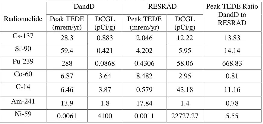
Table 4.2 The Screening analysis peak dose results and DCGL with DandD and RESRAD deterministic code……… 48

Table 4.3 Scaling factors for selected radionuclides at the plant site ……… 50

Table 4.4 The results of estimated concentrations for selected ……… 50

Table 4.5 Human consumption rate of fruits, vegetables, and grains(g/d per capita)… 56 Table 4.6 Human consumption rate of meat, animal products, fish(g/d) ……… 56

Table 4.7 The Kd values in loam soil (L/kg)……… 61

Table 4.8 Soil-to-plant transfer factor for Cs in loam (Bq/kg/Bq/kg)… ……… 62

Table 4.9 Soil-to-plant transfer factor for Sr in loam (Bq/kg/Bq/kg)… ……… 63

Table 4.10 Parameter used in DandD and RESRAD (Site-specific)… ……… 64

Table 4.11 Parameters after Bayesian Updating……… 74

Table 4.12 Dose results with updated information for Cs-137……… 76

Table 4.13 Dose results with updated information for Sr-90……… 77

Table 4.14 Dose results with updated information for Pu-239……… 78

Table 4.15 Dose results with updated information for Co-60……… 79

Table 4.16 Dose results with updated information for C-14……… 80

Table 4.17 Dose results with updated information for Am-241……… 81

Table 4.18 Dose results with updated information for Ni-59……… 82

Table 4.19 Relative important parameters for different radionuclides in analysis (DandD)… ……… 83

Table 4.20 Dose results with updated information for Cs-137……… 85

(9)

Table 4.22 Dose results with updated information for Pu-239……… 87

Table 4.23 Dose results with updated information for Co-60……… 88

Table 4.24 Dose results with updated information for C-14……… 89

Table 4.25 Dose results with updated information for Am-241……… 90

Table 4.26 Dose results with updated information for Ni-59……… 91

Table 4.27 Relative important parameters for different radionuclides in analysis (RESRAD)… ……… 92

Table 4.28 Dose results and DCGL for selected parameter (DandD)… ……… 93

Table 4.29 Dose results and DCGL for selected parameter (RESRAD)……… 95

Table 4.30 Utility analysis for prior information (DandD)……… 99

Table 4.31 Utility analysis for prior information (RESRAD)……… 99

Table 4.32 Utility analysis for posterior information (DandD)……… 100

Table 4.33 Utility analysis for posterior information (RESRAD)… ……… 101

Table 4.34 Conditional value of information results (DandD)… ……… 103

(10)

LIST OF FIGURES

Figure 1.1 NRC’s Hierarchy of Dose Assessment Modeling Approaches

(NUREG/CR-5512) ……… 3

Figure 1.2 Decommissioning and license termination framework……..……… 8

Figure 2.1 Prior PMF of parameter θ……… 15

Figure 2.2 Continuous prior distribution of parameter θ……… 17

Figure 4.1 A nuclear power plant site boundary and owner-controlled area used in the study……… 44

Figure 4.2 Distribution for the thickness of unsaturated zone……… 51

Figure 4.3 Distribution for the Annual precipitation rate……… 52

Figure 4.4 Distribution for saturated zone hydraulic conductivity……… 53

Figure 4.5 Distribution for total porosity……… 54

Figure 4.6 Distribution for density……… 55

Figure 4.7 Distribution for consumption rate – leafy……… 57

Figure 4.8 Distribution for consumption rate – grain……… 58

Figure 4.9 Distribution for consumption rate – fruits, vegetables, and grains………… 58

Figure 4.10 Distribution for consumption rate – beef……… 59

Figure 4.11 Distribution for consumption rate – poultry……… 60

Figure 4.12 Distribution for consumption rate – meat and poultry……… 60

Figure 4.13Bayesian updating for the thickness of unsaturated zone……… 66

Figure 4.14 Bayesian updating for total porosity……… 67

Figure 4.15 Bayesian updating for density……… 68

Figure 4.16 Bayesian updating for Kd: Cs-137……… 69

Figure 4.17 Bayesian updating for Kd: Sr-90……… 70

Figure 4.18 Bayesian updating for Kd: Pu-239……… 70

Figure 4.19 Bayesian updating for Kd: Co-60……… 71

Figure 4.20 Bayesian updating for Kd: C-14……… 71

Figure 4.21 Bayesian updating for Kd: Am-241……… 72

Figure 4.22 Bayesian updating for Kd: Ni-59……… 72

(11)

Figure 4.24 Dose values over time in year for default distributions (Sr-90)………… 77 Figure 4.25 Dose values over time in year for default distributions (Pu-239)………… 78 Figure 4.26 Dose values over time in year for default distributions (Co-60)………… 79 Figure 4.27 Dose values over time in year for default distributions (C-14)… ……… 80 Figure 4.28 Dose values over time in year for default distributions (Am-241)… …… 81 Figure 4.29 Dose values over time in year for default distributions (Ni-59)… ……… 82 Figure 4.30 Dose over time in year and CDF of peak dose for default distributions

(Cs-137)……… 85

Figure 4.31 Dose over time in year and CDF of peak dose for default distributions

(Sr-90)… ……… 86

(Pu-239)……… 87

(Co-60)……… 88

(C-14)… ……… 89

(Am-241) ……… 90

(Ni-59) ………91

Figure 4.37 Uncertainty in dose predictions due to the uncertainty in the density

of unsaturated zone ……… 94 Figure 4.38 Uncertainty in the DCGL due to the uncertainty in the density

of unsaturated zone……… 95 Figure 4.39 Updated posterior function with new likelihood function

-density of unsaturated zone……… 106 Figure 4.40 Comparison among different number of samples……… 107 Figure 4.41 Updated posterior function with new likelihood function

-precipitation rate……… 108

Figure 4.42 Updated posterior function with new likelihood function

(12)

Bayesian Analysis for the Site-Specific Dose Modeling in

Nuclear Power Plant Decommissioning

1. Introduction

1.1 Environmental Decision Making in Nuclear Power Plant Decommissioning

Decommissioning is the process of closing down a facility. For a nuclear facility, it means to remove a facility or site safely from service and reduce residual radioactivity to a level that permits: (a) release of the property for unrestricted use and termination of the license; or (b) release of the property under restricted conditions and termination of the license. Currently several nuclear power plants in the United States are in the decommissioning phase [NRC Website, 2001].

One of the essential issues in nuclear power plant decommissioning is to ensure that any remaining radioactivity at a decommissioned site should not pose unacceptable risk to any member of the public after the release of the site. Based on the consideration of acceptable risk, the levels of allowable residual contamination should be determined and the site must be cleaned accordingly [Beyeler, W.E., and Davis, P.A., et al., 1996]. The safety and cost of a decommissioning project will be controlled predominately by this allowable residual contamination level.

(13)

predictive analyses, uncertainty is present in almost every aspect of dose assessment including the conceptualization of the site, assumptions on human exposure pathways, implementation of mathematical models, and development of data for model parameters [Beyeler, W.E., and Brown, T.J., et al., 1998][Kamboj, S., and LePoire, D., et al., 2000]. This uncertainty can be very large depending upon the amount of effort given to the characterization of site and related parameters. Decisions on the required site-cleanup efforts or the acceptance of the residual risk at the site must be made in the light of the uncertainties in the predictive analysis. This renders the problem a classic example of a risk-based decision making problem or an environmental risk management problem. Therefore, analysis of the problem requires a systematic decision analysis framework along with the use of dose assessment methodologies.

The characterization of uncertainty is critical in the application of predictive models to risk-based decision making in nuclear power plant decommissioning. Uncertainties arise due to (i) the limited scientific understanding of important processes; (ii) the inadequacy of mathematical representations which require simplifications of physical processes and their temporal and spatial aggregation; and (iii) the limited ability to measure model parameters and inputs. A systematic analysis of these uncertainties is needed to determine their impact on model predictions and decisions that might be based upon these predictions.

1.2 U.S. NRC’s Regulations and Approaches to Dose Assessment

(14)

background radiation results in a Total Effective Dose Equivalent (TEDE) to an average member of the critical group does not exceed 25 mrem (0.25 mSv) per year, including that from groundwater sources of drinking water, and the residual radioactivity has been reduced to levels that are as low as reasonably achievable (ALARA) [NRC Website-CFR, 2001].

If the dose assessment for a given site determines that the residual radioactivity will result in a dose greater than the regulatory limit, measures must be taken to reduce or remove the radioactivity from the contaminated radioactive material. These measures could include: (a) removing the source material; (b) treating the material to reduce the contamination, (c) letting the material radioactively decay away, or (d) covering the contamination to shield or attenuate the radiation emitted.

Dose assessment relies on the efforts of site characterization and the tools for modeling and analysis. In dose assessments, a reasonable treatment of uncertainty is needed to provide the regulator with the confidence that the actions taken and the decision made to terminate the facility license are consistent with the regulations.

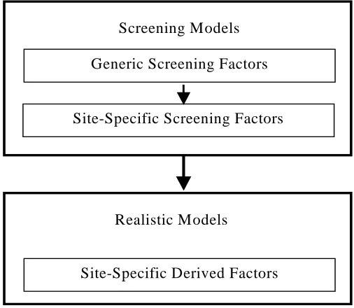
The NRC’s hierarchy of dose assessment modeling is shown in Figure 1.1 [Kennedy, W.E., Jr., and Strenge, D.L., 1992].

Screening Models Generic Screening Factors

Site-Specific Screening Factors

Realistic Models

Site-Specific Derived Factors

(15)

During the development of the dose assessment approach, models, scenarios, and parameters should be defined which were expected to be “reasonably conservative”. The models and scenarios are specifically defined such that they would not be “bounding” or unrealistic, while still generally overestimating rather than underestimating potential dose. The model parameters in dose modeling are also evaluated to exclude bounding or unrealistic assumptions. The purpose is two-fold: first, to provide a basis for screening; second, to provide information for more complex decommissioning situations where a clear understanding of the modeling assumptions and construction of the parameters is needed to support changes that lead to more realistic dose assessments. To capture the dose to a critical group, NRC developed a set of exposure scenarios that should serve as conservative representations of a multitude of possible exposure scenarios to humans. These include industrial occupancy, renovation, residential farmer, and drinking water. The purposes and the specific models among those scenarios are different for dose assessment.

The NRC methodology is based on the premise that screening dose assessments are performed with little site-specific information [Kennedy, W.E., Jr., and Strenge, D.L., 1992]. The screening would comply with more restrictive criteria, but would do so based on a decision to not expend resources for a more realistic dose estimate, and would have high assurance that the criteria would be met. However, for more complex situations or more realistic analyses, the methodology ensures that as more site-specific information is incorporated, the uncertainty is reduced and the estimate of the resulting dose generally decreases. This provide assurance that obtaining additional site-specific information is worthwhile because it ensures that a more “realistic” dose assessment will not generally result in a dose higher than that estimated using screening.

(16)

simple assumptions and default models and parameter values that are intended to be prudently, but not excessively, conservative. Level 1 calculations are intended to produce generic dose estimates that are unlikely to be exceeded at real sites. Level 2 screening allows users to adjust certain parameters and eliminate pathways to more closely approximate conditions at their particular site. Level 3 modeling is based on site-specific models and data and is beyond the scope of the screening methodology. The methodology is designed so that conservatism is reduced and the resulting dose decreases as the process moves from one level to the next upper level. For a Level 1 analysis, site-specific source-term data is used with the default models and parameters. A Level 2 analysis implements the default models with site-specific source-term and parameter data. For a Level 3 analysis, site-specific models are developed and implemented with site-specific source-term and parameter data.

Computer codes used in these efforts include DandD and RESRAD [Yu, C., and Zielen, A.J., et al., 1993][Yim, M.S., 1999]. Sandia National Laboratory developed the DandD computer code. DandD provides a structured interface that allows users to apply screening models to estimate doses under four distinct exposure scenarios: industrial occupancy, renovation, residential farmer, and drinking water. Default parameters were selected based on a rigorous analysis such that defensible screening calculations can be made using information about the source. RESRAD was developed by Argonne National Laboratories in the late 80s, and has been widely used by the Department of Energy (DOE), Environmental Protection Agency (EPA), and the nuclear power industry to estimate doses from residual radioactive material and set site-specific clean modeling platforms, but they are not specifically organized for implementation of the four exposure scenarios given in NUREG/CR-5512 [NRC Report, 1998]. Previous version of RESRAD is also a deterministic code used to perform dose analysis. RESRAD new version, version 6.0, was released in August 2000 for the probabilistic dose analysis by using parameter distributions incorporated in RESRAD code.

(17)

1.3 U.S. NRC’s Decision Framework for Plant Decommissioning

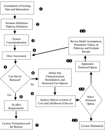
A logical, consistent decision process is viewed as a useful tool by the NRC that will support the planning of decommissioning activities and regulatory review of license termination requests along with the use of dose assessment. To support this process, a decision methodology, or framework, is used to support implementation of the dose assessment requirements [NRC Draft NUREG 1549, 1998][NRC NMSS Decommissioning SRP, Appendix C, 2000].

The steps and decision points of the decision framework support assessment of the entire range of dose modeling options from which a licensee may choose, whether it involves using generic screening parameters, changing parameters, or modifying pathways or models. The decision framework, including its steps and decision points, is discussed in this section.

To facilitate the preparation and evaluation of the dose assessments, a phased approach to decision-making for license termination was adopted because of the very wide range of levels of contamination and complexity of analysis and potential remediation necessary at NRC-licensed sites. The phased approach consists of generic screening analysis and of making use of site-specific information as appropriate. Is it worthwhile putting resources to reduce the source level according to the results of generic screening or spend some more efforts to seek site-specific information for more realistic dose analysis? By using decision framework, the risk management decision can be best described and made. These phases are described in broad terms below:

(a) Generic Screening: In this phase, licensees would demonstrate compliance with the dose criteria of the rule by using: (i) pre-defined models, and (ii) generic screening parameters.

(18)

provide the licensee with a simple method to demonstrate compliance using little site-specific information.

The pre-defined models and generic screening parameter distributions are used to calculate a reasonably conservative range of doses that the average member of the screening group could receive. This information was used to develop default deterministic parameters for the DandD model.

(b) Use of Site-Specific Information as Appropriate: if compliance cannot be demonstrated using generic screening analysis, then licensees should proceed to the next phase of analysis in which defensible site specific values are obtained and applied. Examples of site-specific features that may require modeling beyond the defaults include (but are not limited to) known groundwater contamination, large quantities of contamination material (such as slag piles), or buried wastes. Depending on the complexity of the site contamination, the licensee can use site-specific:

(i) By replacing generic screening parameters with site-specific parameter values to allow site-specific factors to be taken into account. Thus, the dose estimates would be more realistic. The models can be pre-defined models. Or

(ii) By using site-specific model assumptions;

(iii) By using some combination of a and b and also remedying the site;

(iv) By using some combination of a, b, and c, and also restricting use of the site. In any of the cases (i) – (iv), site-specific data are used to support modifying or eliminating a particular scenario or pathway, or to demonstrate that a parameter or group of parameters can be better represented by site-specific values. Alternative exposure scenarios may be appropriate based on site-specific factors that affect the likelihood and extent of potential future exposure to residual radioactivity. Thus use of dose assessment for these situations can range from fairly simple site assessments to fairly complex analyses.

(19)

Assimilation of Existing Data and Information

Scenario Definition/ Pathway Definition

System Conceptualization

Dose Assessment

Can Site be Released?

ALARA Requirements

License Termination and Sie Release

Define Site Characterization Remediation, and Restricted Use Options

Analyze Options in terms of Cost and Likelihood of Success

Revise Model Assumptions, Parameters Values, & Pathways and Evaluate

Results

Implement Preferred Option

Select Preferred

Option

License Maintained

u

v

w

x

u

v

uu

ut

uw

y

|

z

}

{

Yes

No

(20)

The framework is designed such that the level of complexity and rigor of analysis conducted for a given site should be commensurate with the level of risk that the site poses. Although use of the framework would normally encompass steps 1 through 5, and steps 6 and 7, the amount of work that goes into each of these steps should be based on the expected levels of contamination and the health risks they pose. Note that in this framework, all sites may start at the same level of very simple analyses (not a requirement for successful implementation), but it is expected that only certain sites would progress to very complex dose assessment and options analyses. Some sites may not need to conduct any options analyses (step 8) and some sites may need to evaluate a limited set of relatively simple and inexpensive options. For example, a site with a source of contamination that is obviously simple to remove would not spend time analyzing large suites of alternative data collection and remediation options. On the other hand, a site with high levels of contamination that are widely distributed may use his process to analyze a variety of simple and complex options to define the best decontamination and decommissioning strategy. Thus, the approach ensures that efforts and expenses would be commensurate with the level of risk posed by the site.

The decision framework, described in NUREG-1549, is illustrated in Figure 1.2. The framework can be used throughout the decommissioning and license termination process for sites ranging from the more simple sites to the most complex or contaminated sites.

Step 1: The first step in a dose assessment involves gathering and evaluating existing data and information about the site, including the nature and extent of contamination at the site. Often, minimal information is all that is needed for initial screening analyses. Specifically, information is needed to support the decision that the site is simple and is qualified for screening analysis. However, all information about the site that is readily available should be used. This step also includes definition of the performance objectives that must be met in order to demonstrate compliance with decommissioning criteria.

(21)

the NRC has already defined the generic scenarios and pathways for screening. For site-specific analysis mode, DandD and RESRAD/RESRAD-BUILD codes may be used, in addition to other codes. These codes should allow the user to both select, and deselect, exposure pathways if certain pathways are not considered relevant due to site conditions.

Step 3: Once scenarios are defined and exposure pathways identified, a basic conceptual understanding of the system is developed, often based on simplifying assumptions regarding the nature and behavior of the natural systems. System conceptualization includes conceptual and mathematical model development and assessment of parameter uncertainty. Using DandD for generic screening, the NRC has pre-defined conceptual models for the scenarios along with default parameter distribution. For site-specific analysis the DandD and/or RESRAD/RESRAD BUILD conceptual model can be used after verification that the actual site conceptual model is compatible with the conceptual model of the code used.

Step 4: This step involves the dose assessment or consequence analysis, based on the defined scenarios, exposure pathways, models, and parameters distributions. For generic screening, reviewers can accept look-up table and use the generic models and default parameter probabilistic density functions (PDFs), simply by running DandD with the appropriate site-specific source term, leaving all other information in the software unchanged. Site-specific assessments allow the user to use other codes and change pathways and parameter distributions based on data and information obtained from the site.

(22)

percentile value of dose is less than 25 mrem/yr. If the results are below the limit, the licensee proceeds with step 6 and 7 to demonstrate ALARA requirements and initiate the license termination process defined by NRC in other guidance documents.

If the results are ambiguous or they clearly exceed the performance objective, proceed to step 8 and 9.

Step 8: Full application of the decision framework involves defining all possible options the licensee might address in order to defend a final set of actions needed to demonstrate compliance with license termination criteria. Options may include acquiring more data and information about the site and source of contamination in order to reduce uncertainty about the pathways, models, and parameters and thus reduce the calculated dose; reducing actual contamination through remediation actions; reducing exposure to radionuclides through implementation for land-use restrictions; or some combination of these options.

Step 9: All of the options identified in step 8 are analyzed and compared in order to optimize selection of a preferred set of option to go forward with. This options analysis may consider cost of implementation, likelihood of success (and the expected costs associated with success or failure to achieve the desired results when the option is implemented), timing considerations and constraints, and potentially other quantitative and/or qualitative selection criteria.

(23)

options exist at this time, the licensee may decide to defer actions at this site (step 13) until circumstances allow re-visiting license termination actions. Step 11: Under step 11, the preferred option is implemented. The licensee commits

resources to obtain the information necessary to support revisions to the parameters identified in step 8 and 9.

Step 12: Once data are successfully obtained, the affected parameters for the pre-defined models are revised as appropriate. Also, data may support elimination of one or more of the exposure pathways in the pre-defined scenarios. Once the pathways and parameters are revised, the user would re-visit steps 4 and 5 to determine the impact of the revisions on demonstrating compliance with the performance objectives. If met, the user proceeds to steps 6 and 7. If the performance objective is still exceeded, the assessor returns to steps 8 and 9 to analyze remaining options to proceed.

1.4 Objectives and Organization of the Thesis

Although the NRC’s approach provides the conceptual framework for the use of dose assessment, actual use of site-specific dose assessment requires deeper understanding of the problem, dose assessment, the data collection efforts, and their relationships.

The objective of this thesis is to demonstrate the methodologies of site-specific dose assessment for nuclear power plant decommissioning with the use of Bayesian analysis. An actual decommissioning plant site is used as a test case for the analyses. More specific objectives are:

(1) To identify key parameters of importance in site-specific dose assessment as the focus of site-specific data collection efforts.

(24)

(3) To demonstrate the use of site-specific data along with the existing information with Bayesian approach based on the characterization of uncertainties of major parameters in dose assessment.

(4) To demonstrate the usefulness of site-specific data in both deterministic and probabilistic dose assessment.

(5) To demonstrate the methodology of Value of Information (VOI) Analysis and to examine the usefulness of the approach in the site-specific dose assessment for nuclear power plant decommissioning.

(6) To examine the importance of addressing the uncertainty in the definition of likelihood function for the Bayesian VOI analysis.

Only the residential farmer scenario was used in the analyses given that the residual contamination was in the surface soil. Both the DandD and RESRAD computer codes were used for the analyses in this thesis.

The organization of this thesis is as follows: Chapter 2 describes the basic theory of Bayesian updating and the methods used in parameter updating. Some definitions and theories applied for value of information and reliability analysis are also presented.

Chapter 3 concentrates on the collection and analysis of input parameters for the DandD and RESRAD codes. The first section of this chapter discusses the key parameters in nuclear power plant decommissioning dose assessment. Then the default inputs for both codes are discussed. The data analysis in this chapter is to provide the prior information required by the Bayesian updating in Chapter 4.

Chapter 4 describes the development of site-specific data for major parameters in dose assessment by using various sources of information, the results of Bayesian updating, the application of the value of information analysis and its results. The issue of the selection of likelihood function in the Bayesian updating is also discussed.

(25)

2. Bayesian Analysis for Site-Specific Dose Modeling

Accurate estimates of parameters require large amounts of data. When the observed data are limited, as is often the case in engineering, the statistical estimates have to be supplemented (or may even be superseded) by judgmental information. With the classical statistical approach there is no provision for combing judgmental information with observational data in the estimation of the parameters.

The Bayesian method approaches the estimation problem from another point of view [Ang, A. H-S, and Tang, W. H., 1975]. In this case, the unknown parameters of a distribution are assumed (or modeled) to be also random variables. In this way, uncertainty associated with the estimation of the parameters can be combined formally (through Bayes’ theorem) with the inherent variability of the basic random variable. With this approach, subjective judgments based on intuition, experience, or indirect information are incorporated systematically with observed data to obtain a balanced estimation. The Bayesian method is particularly helpful in cases where there is a strong basis for such judgments. The basic concepts of the Bayesian approach are discussed in the following sections [Patwardhan, A., and Small, M. J., 1992][Small, M. J., 1997].

2.1 Bayesian Analysis 2.1.1 Discrete Case

The Bayesian approach has special significance to engineering design, where available information is invariably limited and subjective judgment is often necessary. In the case of parameter estimation, the engineer often has some knowledge (perhaps inferred intuitively from experience) of the possible values, of a parameter; moreover, he may also have some intuitive judgment on the values that are more likely to occur than others. For simplicity, suppose that the possible values of a parameter θ were assumed to be a set of discrete values θi, i = 1, 2, …, n, with relative likelihood (Probability Mass

Function-PMF) pi = P(Θ = θi) as illustrated in Figure 2.1 (Θ is random variable whose

(26)

θ1 θ2 θ3 θ_n

p1

p2

p3

pn

pi= P (Θ=θi)

Figure 2.1 Prior PMF of parameter θ

Then if additional information becomes available (such as the results of a series of tests or experiments), the prior assumptions on the parameter θ may be modified formally through Bayes’ theorem as follows.

Let ε denote the observed outcome of the experiment. Then applying Bayes’ theorem, we obtain the updated PMF for θ as

n i P P P P P _n i i i i i

i 1,2,...,

) ( ) | ( ) ( ) | ( ) | ( 1 = = Θ = Θ = Θ = Θ = = Θ

∑

= ε θ θ θ θ ε ε

θ (2.1)

The various terms in Eq. 2.1 can be interpreted as follows: )

|

( _i

P ε Θ=θ = the likelihood of the experimental outcome ε if Θ = θi; that is, the

conditional probability of obtaining a particular experimental outcome assuming that the parameter is θi.

)

( _i

P Θ=θ = the prior probability of Θ = θi; that is, prior to the availability of the

experimental information ε )

| ( θ_i ε

P Θ= = the posterior probability of Θ = θi; that is, the probability that has

(27)

Denoting the prior and posterior probabilities as

P

’

(

Θ

=

θ

_i

)

and

P

’

(

Θ

=

θ

_i

)

, respectively, Eq. 2.1 becomes

∑

= = Θ = Θ = Θ = Θ = = Θ _n i i i i i i P P P P P 1 ) ( ’ ) | ( ) ( ’ ) | ( ) ( ’ ’ θ θ ε θ θ ε

θ (2.1a)

Eq. 2.1a, therefore, gives the posterior probability mass function of Θ.

The expected value of Θ is then commonly used as the Bayesian estimator of the parameter; that is,

∑

= = Θ = Θ = n i i iP E 1 ^ ) ( ’ ’ ) | ( ’ ’ ε θ θ

θ (2.2)

We may point out that in Eq. 2.2 observational data and judgmental information are both used and combined in a systematic way to estimate the underlying parameter.

In the Bayesian framework, the significance of judgmental information is reflected also in the calculation of relevant probabilities. In the case above, where subjective judgments were used in the estimation of the parameter θ, such judgments would be reflected in the calculation of the probability, for example, P(X ≤ a), through the theorem of total probability using the posterior PMF of Eq. 2.1a. That is,

∑

=

≤

Θ

=

Θ

=

≤

n 1 i i i

)

P

’

(

)

|

a

X

(

P

)

a

X

(

P

θ

(2.3)

This represents the up-to-date probability of the event (X ≤ a) based on all available information. It may be emphasized that in Eq. 2.3 the uncertainty associated with the error of estimating the parameter (as reflected in

P

’

(

Θ

=

θ

_i

)

) is combined with the inherent variability of the random variable X.

2.1.2 Continuous Case

(28)

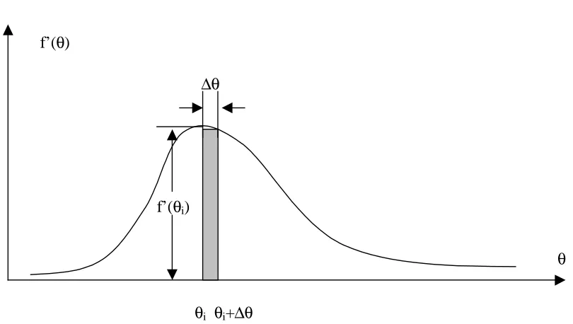
to assume the parameter to be a continuous random variable in the Bayesian estimation. In this case we develop the corresponding results, analogous Eqs. 2.1 through 2.3, as follows:

∆θ

θi θi+∆θ

θ f’(θ)

f’(θi)

Figure 2.2 Continuous prior distribution of parameter θ

Let Θ be the random variable for the parameter of a distribution, with a prior density function

f

’

(

θ

)

shown in Figure 2.2. The prior probability that θ will be between θi and θi+∆θ then is

f

’

(

θ

_i

)

∆

θ

. Then, if ε is an observed experimental outcome, the prior

distribution

f

’

(

θ

)

can be revised in the light of ε using Bayes’ theorem, obtaining the posterior probability that θ will be in (θi, θi+∆θ) as

∑

=

∆

=

∆

_n

1 i

i i

i

)

(

’

f

)

|

(

P

)

(

’

f

)

|

(

P

)

(

’

f

θ

ε

θ

ε

θ

(29)

∫

−∞∞

=

θ

ε

θ

ε

θ

d

)

(

’

f

)

|

(

P

)

(

’

f

)

|

(

P

)

(

’

f

(2.4)

The term

P

(

ε

|

θ

)

is the conditional probability or likelihood of observing the

experimental outcome ε assuming that the value of the parameter is θ. Hence

P

(

ε

|

θ

)

is a function of θ and is commonly referred to as the likelihood function of θ and denoted L(θ). The denominator is independent of θ; this is simply a normalizing constant required to make

f

’

(

θ

)

a proper density function. Eq. 2.4 then can be expressed as

)

(

’

f

)

(

kL

)

(

’

f

θ =

θ

(2.5)

where the normalizing constant

k

=

[

∫

₋∞_∞

P

(

ε

|

θ

)

f

’

(

θ

)

d

θ

]

−1; and L(θ) = the likelihood of observing the experimental outcome ε assuming a given θ.

We observe from Eq. 2.5 that both the prior distribution and the likelihood function contribute to the posterior distribution of θ. In this way, as in the discrete case, the significance of judgment and of observational data are combined properly and systematically; the former through

f

’

(

θ

)

and the latter in L(θ).

Analogous to the discrete case, Eq. 2.2, the expected value of θ is commonly used as the point estimator of the parameter. Hence the updated estimate of the parameter θ, in the light of observational data ε, is given by

∫

−∞∞

=

θ

ε

θ

’

E

(

|

)

f

’

(

)

d

^

(2.6)

The uncertainty in the estimation of the parameter can be included in the calculation of the probability associated with a value of the underlying random variable. For example, if X is a random variable

∫

−∞∞

≤

=

≤

a

)

P

(

X

a

|

θ

)

f

’

(

θ

)

d

θ

X

(

P

(2.7)

(30)

2.2 Combining Information – Bayesian Updating

Combining information is necessary and important in site-specific dose assessment for nuclear power plant decommissioning. As new pieces of information become available through site investigations, the new data should be properly combined with the prior-existing body of knowledge to improve the dose assessment. Bayesian updating is very useful for this purpose. This section discusses different ways of combining information within the Bayesian analysis framework [Ang, A. H-S, and Tang, W. H., 1975].

2.2.1 Combining with Conjugate Pair

This is an ideal case for Bayesian updating. It assumes that the site-specific information are all obtained with same or similar approaches as the national data (prior information) do. Then the site-specific information can be used to update the prior information with Bayesian method. This case in fact simply assumes the distribution of site-specific information as the likelihood function. It’s a simple combination of two known PDFs into one posterior PDF. For normal/lognormal distributed prior, likelihood functions, there are analytical results for the posterior distribution with those conjugate distributions. As for normal pairs, the posterior is normal, its statistical parameters µ”

and σ” are:

Mean: ₂ ₂

2 2

’ ’ ’

’ ’

σ σ

σ µ σ µ µ

+ ⋅ + ⋅

= (2.8)

Standard deviation: ₂ ₂

2 2 ’

’

’ ’

σ σ

σ σ σ

+ ⋅

= (2.9)

where µ’, σ’ are the parameters for prior distribution, µ, σ are the parameters for site-specific distribution. Similarly for lognormal pairs, by taking logarithmic transform, the parameters are:

(31)

2 ln 2 ln 2 ln ln 2 ln ’ ln ’ ’ ln ’ ’ σ σ σ µ σ µ µ + ⋅ + ⋅

= (2.10)

Standard deviation (after logarithmic transform):

2 ln 2 ln 2 ln 2 ln ’ ’ ln ’ ’ σ σ σ σ σ + ⋅

= (2.11)

Use Bayesian conjugate pairs for normal and lognormal distributions (the most common types of distribution in engineering analysis), the updated results for each parameter can be obtained.

2.2.2 Combining with Sampling from Normal Population

If the experiment outcome ε in Eq. 2.4 is a set of observed values x1, x2, …, xn,

representing a random sample from a population X with underlying density function fX(x), the probability of observing this particular set of values, assuming that the

parameter of the distribution is θ, is

∏

=

= n

i

X x dx

f P 1 ) | ( ) | (ε θ θ

Then, if the prior density function of θ is f’(θ), the corresponding posterior density function becomes, according to Eq. 2.4,

) ( ’ ) ( ) ( ’ ] ) | ( [ ) ( ’ ] ) | ( [ ) ( ’ ’ 1

1 θ θ

θ θ θ

θ θ

θ kL f

d f dx x f f dx x f f _n i i X n i i X = =

∫ ∏

∏

∞ ∞ − ₌

= _(2.12)

in which the normalizing constant ‘k’ is

1 1 ] ) ( ’ )) | ( ( [ ∞ − ∞ − =

∫ ∏

= f x θ f θ dθ

k

n

i

i X

and the likelihood function L(θ) is the product of the density function of X evaluated at x1, x2, …, xn, or

∏

= = n i i X x f L 1 ) | ( )

(32)

In the case of a Gaussian population with known standard deviation σ, the likelihood function for the parameter µ, according to Eq. 2.13, is

∏

= = =     − − = n i i n i i x N x L 1 1 2 ) , ( ) 2 1 exp( 2 1 ) ( σ σ µ σ π

µ µ (2.14)

where Nµ(xi, σ) denotes the normally distributed density function of µ with mean value xi

and standard deviation σ. It can be shown that the product of m normal density functions with respective means µi and standard deviations σi is also a normal density function with

mean and variance

∑

= = = ₌ = _m i i m i i m i i i and 1 2 2 1 2 1 2 1 1 *) ( 1 * σ σ σ σ µ µ

For the samples obtained from the same site-specific distribution, they have the same standard deviation. Therefore the likelihood function L(µ) becomes

) , ( ) 1 , 1 ( ) ( 2 2 1 2 n x N n n x N L n i s σ σ σ σ µ = µ = µ

∑

= _(2.15)

where x is the sample mean.

2.3 Model Uncertainty Analysis - Bayesian Monte Carlo (BMC)

(33)

temporal averaging, and imperfect model representation. For example, for unbiased measurements with a normally distributed error, the likelihood of an observation is given as:

) 2

1 exp( 2

1 ) (

) | (

2

   

  − −

= − =

ε

ε σ

σ π

θ ε

k k

Y O f

Y O L

(2.16)

where O is observations, Yk is the model predictions, and

2 ε

σ

= the observation error variance.

The selection of the appreciated error structure for the likelihood function is a key consideration for the Bayesian analysis; it requires a careful consideration of the relationship between the model predictions and the observed data. For example, when the relationship is direct, i.e., when model predictions and observed data are available at the same level of temporal and spatial aggregation, then a likelihood estimate based on field and laboratory measurement error is appropriate. In many applications, the correspondence between observed data and model predictions is less direct. In these cases, the error variance in Eq. 2.16 must incorporate the effects of the un-represented variances as well as the error associated with inaccuracy in the measurement methods used to obtain the data.

An additional complication arises from the independent assumption, which is inherent in the use of Eq. 2.13. This assumption, though commonly employed, is often inappropriate. The correlations in the observed data, model predictions, and the difference between them, can violate the independence assumption, causing the information content of an observed dataset to be reduced. In most cases, an approach is employed: the likelihood is defined using statistics that represent the aggregate relationship between the observed data and the model.

(34)

2.4 Bayesian Decision Theory and Reliability Analysis

Reliability certification [Papazoglou, I. A., 1999] or reliability demonstration addresses the need to demonstrate that the reliability related characteristics of an engineered technological system meet certain requirements. The most common form of these requirements is that the reliability of a system, i.e., the probability that the system will perform a required function under stated conditions and for a stated period of time, is greater than a given value. The reliability of a system is estimated from existing or acquired information referring either to its performance as a whole or to the performance of its parts or components. If the reliability of a system considered as a single component is known with certainty, then the certification follows from direct comparison with the required reliability value. Similarly straightforward is the certification in the case where the reliability of the components of the system is known along with their logical interconnection in the system. In the latter case the reliability of the system is expressed as a function of parameters referring to the stochastic behavior of the components.

(35)

2.4.1 Axiomatic Definitions

Bayesian decision theory is a formal mathematical structure that guides a decision maker in choosing a course of action in the face of uncertainty about the consequences of that choice. The course of action recommended by the theory is one which is consistent with the decision maker’s preference for various consequences and the uncertainties involved in the problem. More formally, the Bayesian decision problem, as it relates to reliability analysis, is defined in terms of the following:

1. A space A of two possible actions which are available to the decision maker;

{

a1, a2

}

A=

where action a1 is “Accept the system” and action a2 is “Do not accept the system”. The

meaning of the statement “accept the system” is that the system is accepted with respect to its reliability and from the decision maker’s point of view. For a producer “accept” means produce the system at the assessed reliability level, for a buyer “accept” means buy it. A similar meaning is assigned to the statement “Do not accept” or “reject” the system.

2. A space of possible “states of the world”, I =

{ }

R , where I is the set of the possible values of the reliability of the system R, and therefore I consists of the interval of the real line (0,1).

3. A family of possible experiments E =

{ }

e . One of these experiments can be used to obtain more information about the state of the world. E includes a dummy experiment which consists of making an immediate decision with no experimentation. In the context of this analysis an experiment consists in observing a system or components of the system and recording their reliability related performance.

4. A space of possible outcomes Z =

{ }

z for the experiments in E. In the reliability context outcomes of experiment consist of times of observation and successful or not in the completion of the mission during these times.

(36)

have a certain consequence to the decision maker that chose this particular course of action.

The axioms and the basic theorems of Bayesian decision theory, can be summarized as follows:

Proposition 1. There exist a preference relation ½ over the set of all consequences

{ }

c

C = such that if ci and cj belong to C then one of the following three alternatives is

true.

(1). ci½cj (ci “is preferred to” cj).

(2). cj½ci (cj “is preferred to” cj).

(3). Both (1) and (2) (indifference between ci and cj).

Proposition 2. The decision maker can express his preference for consequences by a

real-valued function u(.) such that ci½cj if and only if u(ci) > u(cj). The function u(.) is

called the utility function.

Proposition 3. The existing uncertainties about the reliability of the system and the

relative likelihood of the experimental outcomes can be expressed by means of a

probability measure ( , )

~ ~

z R

P on I×Z. From ( , )

~ ~

z R

P one can obtain the marginal

probability measure ( )

~

R

P on I, called the prior probability distribution of the reliability (i.e., prior to experimentation). If an experiment e results in an outcome z, the decision maker’s prior knowledge is modified by means of Bayesian theorem to yield the posterior probability distribution. The reliability of posterior information can be obtained based on the posterior probability distribution function.

From the foregoing it can be shown that if the decision maker is to act consistently with his preference for consequences and the existing uncertainties, he should choose the act that maximizes the expected utility of the consequence of that act, the expectation

being taken with respect to ( , )

~ ~

z R P .

(37)

2.4.2 The Nature of the Utility Function

A general assumption on the nature of the utility function that will be made can be stated in the form of the following proposition.

Proposition 4. The utility function u(c), which is defined on C=E×Z×A×I, can be expressed as the sum of a function us(.,.) on E×Z and a function u(.,.) on A×I,

) , ( ) , ( )

(c u e z u a R

u = _s + (2.17)

Utility function us(e,z) refers to the sampling part and describes the preferences of

the decision maker on choosing experiment e and observing outcome z. Utility function u(a,R) describes the preferences of the decision maker on deciding a for a system with reliability R. The general characteristics of u(a,R) are as follows:

1. If act a1 is chosen then it is assumed that a rational decision maker would prefer a

larger reliability than a smaller one, so that

u(a1,R1) ≥ u(a1,R2) if and only if R1 ≥ R2 (2.18)

2. If act a2 is chosen, the decision maker’s preferences could be based on two

different arguments. On one hand, one could argue that once a decision of not accepting the system has been made, no consequence from a particular reliability (small or large) of the system can actually be realized. Therefore the particular value of the reliability of the system that it would have obtained if the system was accepted is unimportant to the decision maker, and the utility function is constant for all R.

I R R constant

R a

u( ₂, )= . ∀ , ∈ (2.19)

On the contrary one could argue that the choice of action a2 (do not accept),

combined with a large reliability that the system would exhibit if adopted represents an opportunity loss for the decision maker, in the sense that the decision maker by choosing action a2 lost the opportunity to accept a reliable system. If this argument

represents the decision maker’s preference then it is obvious that the utility function u(a2, R) does not take the same value for every possible value of R, and further, a

larger reliability (larger opportunity loss) is less preferred to a smaller one (smaller opportunity loss), i.e.,

(38)

It will always be assumed that there exists an “equilibrium” value of the reliability, R0 such that

u(a1,R0) ≥ u(a2,R0) R0∈(0, 1) (2.21)

With regard to the utility function us(e,z) it is usually convenient to think of this

utility in terms of its negative value defined by the following equation,

cs(e,z) = - us(e,z) (2.22)

called the “cost” of performing the experiment e and observing the result z. it is apparent that whatever the point of view, both us(e,z) and cs(e,z) depend exclusively on the nature

of the space E.

2.4.3 Prior Analysis

As it was stated repeatedly in the foregoing, the purpose of decision theory is to suggest the best course of action, i.e., the optimum experiment e* and the optimum act a* given the results of this experiment. Before examining how the information resulting from an experiment can be used and which experiment should be selected, it would be helpful to examine the two limiting cases of experimentation: (1) the dummy experiment (called also the null experiment) which consists of no experimentation at all; and (2) the ideal experiment which, if performed, would yield perfect information that is, eliminate any uncertainties about the reliability of the system.

The reason for analyzing the null experiment is that this experiment represents an actual alternative to the decision maker. It is possible that the decision maker will decide on the basis of the existing information only, available in terms of the prior probability measure on I. Further, exactly the same analysis is applicable after an experiment has been performed and an outcome z has been observed. The only difference would be that instead of the prior measure p’(R) on I the probability measure P”(R) will be used.

If perfect information were available to the decision maker, then the optimum act aR

(conditional on R) would be,







<

≥

=

0 2

0 1

R

if

only

and

if

a

R

if

only

and

if

a

(39)

The exact value of the reliability of R is not known to the decision maker at the

moment of the decision. With the definitions of the prior expected utilities ’

_

1

u and ’

_

2

u ,

the prior optimum act a* can be written as,











<

≥

=

_{_} ’ 1 _ ’ 1 2 _ ’ 2 _ ’ 1 1

*

u

if

only

and

if

a

u

if

only

and

if

a

_(2.24)

This equation determines the best course of action on the basis of the prior information alone.

2.4.4 The Conditional Value of Sample Information (CVSI)

It is now assumed that the decision maker can perform a real experiment e, which yields information. In other words the results of the experiment will be to “update” the prior measure F’(R) to a posterior measure F”(R) (or the prior PDF f’(R) to a posterior PDF f”(R)). Let az* denote the optimal act after the experiment has been performed and

the outcome z has been observed and with the definition of "

_

1

u and "

_

2

u , the optimal act can be written as,

    < ≥ = _ 1 _ 1 2 _ 2 _ 1 1 " " " " * u u if only and if a u u if only and if a

a _(2.25)

Now the decision maker by choosing: to perform the experiment and to act after observing the outcome according to a”*, instead of choosing: not to perform the experiment and to act according to a’*; has increased his utility after the fact by the following amount ’*)] ( [ "*)] (

[u a E u a E

CVSI ≡ − (2.26)

(40)

         < < > < − < > − > > = ’ ’ " " 0 ’ ’ " " " " ’ ’ " " " " ’ ’ " " 0 _ 2 _ 1 _ 2 _ 1 _ 2 _ 1 _ 2 _ 1 _ 1 _ 2 _ 2 _ 1 _ 2 _ 1 _ 2 _ 1 _ 2 _ 1 _ 2 _ 1 u u and u u if u u and u u if u u u u and u u if u u u u and u u if

CVSI _(2.27)

(41)

3. Site-Specific Dose Assessment – Use of Data

3.1 Dose Assessment for Nuclear Power Plant Decommissioning

Dose assessment is to project the dose to potentially exposed humans from the presence of radioactive source materials. Activities required for a dose assessment include characterizing the source term, developing a conceptual model for a given site, selecting a computer code that is compatible with the site conceptual model, developing supporting input data for the selected computer code, executing the code, and interpreting the results for the necessary decisions. The computer codes that are capable of performing dose assessment for a decommissioning nuclear power plant have been identified by the NRC as described in section 1.2. Therefore, main work to be done in decommissioning dose assessment exercise is to develop an appropriate site conceptual model and prepare appropriate data for the input parameters.

Contamination in a decommissioning nuclear power plant can exist in a wide diversity of conditions. For example, radionuclides in soil can originate from intentional disposal, accidental spill, or long-term accumulation of material deposited from airborne releases during plant operation. The complexity of the environmental setting also influences the potential pathways and components that may need to be considered in modeling human exposures. Therefore, the conceptual model must be broad enough to account for many different, and potentially complex, pathways and conditions for the given residual soil contamination. These potential situations range from simply inhaling air that contains re-suspended contaminated soil to ingesting drinking water from a contaminated well or fish from contaminated surface water, or a variety of plant and animal products that may be grown in the contaminated soil.

(42)

How much? Where do they get water and how much? How much time do they spend on various activities? etc.) Therefore, the type of required input parameters remain the same between different sites. These parameters include physical, behavioral, and metabolic parameters. The physical parameter is classified as any parameter whose value, for a given site and a given group of exposed individuals, would not change if a different group of individuals were considered. All other parameters are behavioral. Within behavioral parameters, a further distinction is made between parameters describing interaction with the site in the context of the scenario, and metabolic parameters. Under the ICRP 43 recommendation [ICRP Publication 43, 1985], values for metabolic parameters would not depend on site conditions nor on the composition of the generic screening group. Distributions were not defined for metabolic parameters. In the residential scenario model, the breathing rate parameters were classified as metabolic.

There are about 222 input parameters required to execute DandD and more than 120 parameters for RESRAD. Therefore developing appropriate input data for all of these parameters is a formidable task. However, the screening methodology developed by NRC provides a default set of input values for these parameters. The NRC’s screening analysis is designed to allow termination decisions to be made without requiring site-specific data. So the data set must therefore be “prudently conservative”, meaning that the dose estimate is likely to decrease if more site information is included in the dose calculation.

For example, for the behavioral parameters, prudently conservative values were established by defining a generic screening group for the scenario. This screening group provides a reasonable upper bound on the behavior of the site-specific critical groups that might be defined in consideration of particular site features. Default values for behavior parameters represent the behavior of the average member of the screening group, and are defined by the average value of the parameter distribution from the efforts of uncertainty characterization for each parameter.

Bayesian Analysis for the Site-Specific Dose Modeling in Nuclear Power Plant Decommissioning

ABSTRACT