On the generalized commuting and non-commuting graphs for metacyclic 3-groups

(1)

On the generalized commuting and non-commuting graphs for

metacyclic 3-groups

Siti Norziahidayu Amzee Zamri

a

_{, Nor Haniza Sarmin}

a,*

_{, Mustafa Anis El-Sanfaz}

b

_{, Hamisan}

Rahmat

a

a _{Department of Mathematical Sciences,Faculty of Science, Universiti Teknologi Malaysia, 81310, UTM Johor Bahru, Johor, Malaysia} sb _{Department of Mathematics, Faculty of Science, University of Benghazi, Libya}

* Corresponding author: nhs@utm.my

Article history

Received 19 February 2017 Accepted 2 August 2017

Abstract

Let G be a metacyclic 3-group and let  be a non-empty subset of G G such that

 







x y, G Glcm x,y 3,xy yx x, y



       . The generalized commuting and non-commuting

graphs of a group G is denoted by _GC _and

,

GN



 respectively. The vertex set of the generalized commuting and non-commuting graphs are the non-central elements in the set  such that

 

GC

 

GN ,

V  V    A where A :g  g g: G. Two vertices in GC are joined by

an edge if they commute, meanwhile, the vertices in GN



 are joined by an edge if they do not commute.

Keywords: Metacyclic 3-groups, commuting graph, non-commuting graph, commute

INTRODUCTION

A finite group G is called metacyclic if it contains a cylic normal subgroup N such that the quotient group G

N is also cyclic. A

metacyclic group with prime power order is called metacyclic p-group. In this research, we consider the metacyclic 3-groups by using the presentation of metacyclic p-groups where p is an odd prime given by (Basri, 2013).

The presentation of metacyclic p-groups where p is an odd prime (Basri, 2013) is divided into two types which we considered as Type 1 and Type 2, given in the following.

Theorem 1: (Basri, 2013) Let G be a non-abelian metacyclic p-group. Then G is one of the following:

(Type 1)

 





, : 1, , , where

is an odd prime and , , , 2 ,

, min 1,

p p p

G a b a b b a a

p

   

     

    



   

  

  

(Type 2)

 





, : 1, , , ,

where is an odd prime and , , , , ,

2 , , min 1,

     

     

         

 

   

 

      

p p p p

G a b a b a b a a

p

Throughout this research, we use these two types of metacyclic p -group presentations, in the case when p is equal to 3 to compute the probability that a metacyclic 3-group fixes a set and apply the results to generalized commuting and non-commuting graphs. In this paper, the

complete graph of n vertices is denoted as Kn,while the null graph is

denoted by K0.

Group action on a set

Since the computation of the probability that an element of a group fixes a set is based on group action, the definition of group action on a set is given as follows (Rotman, 2003):

Definition 1: (Rotman, 2003) Let Gbe any finite group and

X

be a set. A group G acts on

X

if there is a function GX X, such that

i.

 

gh xg hx

 

, g h, G x , X ii. 1Gxx,  x G

THE PROBABILITY THAT A METACYCLIC 3-GROUP FIXES A SET

The probability that a group G fixes a set



The probability that two random elements from a group G

commute is called the commutativity degree. The research on this topic has gathered various interests among researchers in the study of group theory and algebra. Thus, several extensions and generalizations of the commutatativity degree have been introduced. One of the extensions which is called the probability that an element of a group fixes a set was introduced by Omer in 2013 (Omer et al., 2013). A few years later, this probability was extended by El-Sanfaz (El-Sanfaz, 2016) and the new result is given in the following.

(2)

Zamri et al. / Malaysian Journal of Fundamental and Applied Sciences Vol. 13, No. 3 (2017) 181-185 Theorem 2: (El-Sanfaz, 2016) Let G be a finite group and let

 



a b, G G a b 2,ab ba



.

       Let G acts on .Then the

probability that an element of a group G fixes the set  is given as

 





,



:



.

G

g G g

P

G        



Next, the following theorem is used in counting the probability that an element of a group fixes a set under the group action of G on ..

Theorem 3: (El-Sanfaz, 2016) Let G be a finite group and let

 



a b, G G a b 2,ab ba



.

       Let G acts on .Then the

probability that an element of a group G fixes the set  is given by

 

 

 

 ,



G

K P

where K

 

 is the number of orbits under the group action of G on

.

The Set Omega

In this research, the set



is considered as a set of ordered pairs



x y,



in G G such that lcm



x,y



3,

xy



yx

,

and

x



y

.

The

set



can also be written in the form

 







x y, G G: lcm x y, 3,xy yx and x y



.

      

The orbit in a group action

Based on Theorem 2 given by (El-Sanfaz, 2016), in order to compute the probability, we first need to calculate the number of orbit,

 



K before we divide it with the size of the set . Therefore, the definition of the orbit in group action denoted by O x

 

is given in the following definition (Goodman, 2006):

Definition 2: (Goodman, 2006) Let Gacts on a set

X

and xX.

The orbit of x, denoted byO x

 

is the subset of

X

where

  

 : 



 .

O x gx g G X

If a group G acts on

X

by conjugation, the orbit is given by

 



1



: .



  

O x gxg g G X This orbit is also known as the conjugacy classes of x in G.

The probability that a metacyclic 3-group fixes a set Next, the probability that a metacyclic 3-group fixes a set



by conjugation action will be presented. To compute the probability, we used the formula given in Theorem 3, which is the size of orbits dividing the size of the set .

The following theorem shows the probability for metacylic 3-group of Type 1, followed by Type 2:

Theorem 4: Let G be a metacyclic 3-group of Type 1 such that

 

3 3 3

, :   1, ,  

   

G a b a b b a a where    , , ,

2 ,

      and min



1,



. Let



be the set of ordered pairs



x y,





x,y



3,

xy



yx

,

and

.

x



y

If G acts on



by conjugation, then

 

14 , when

1, otherwise.

  

 _{ }

    

 

G

P

Proof: Based on the conditions of parameters in the presentation of metacyclic p-groups, where p is an odd prime of Type 1 such that

, , ,

      2 ,   and min



1,



, there are only four possible cases of value of parameters  , and . That is when     ,           ,   ,   . However, when we compute for all four cases, we found that the value of parameters

, and

   can be grouped into two main cases, which are Case I and Case II. Case I consists of parameters when     , meanwhile

Case II consists of parameters when

, , and .

            

Case I. When     . We give example as we take

3, 2,

    then G a27b91, ,

 

b a a3 . In order to get the set, we first need to find the elements of order 1 and 3. From the computation, we get 9 elements of order 1 and 3 which are

3 18 6 18 3 9 18 6 9 3 9 6

1,b a, ,b a b a a b a b a b, , , , , . Next, we check whether they commute or not, and by following the conditions of the set , we get

36.

  The elements are



    

1,b3 , 1,a18 , , a b a b9 3, 9 6





. By Theorem 3, to compute the probability, we need to find the orbits or conjugacy classes. Since the elements 9 18

1,a and a are in Z G

 

, these elements commute with all elements in .From the computation, we found that there are 14 orbits or conjugacy classes that have different sizes which are 1 and 3. The orbits or the conjugacy classes are listed as



_1,b3_{ } , 1,a18 _{ }, 1,b6_, ,_b a b6, 18 6_



. Thus, we have 14 orbits, i.e.

 

14.

K   By Theorem 3,

 

14 .

G

K

P    

 

Case II. When        ,   , and     . Since all these three types of parameters give the same value of probability, we show only one example which is when     .We take   3,2,

then 27 27

 

3

1, , .

G a b  b a a In order to get the set, we first need to find the elements of order 1 and 3. From the computation, we get 9 elements of order 1 and 3 which are

18 9 9 18 9 18 9 9 18 18 9 18

1,a ,b a a b b, , , ,a b a b, ,a b . Next, we check whether they commute or not, and by following the conditions of the set , we get

36.



    

1,a18 , 1,b9 , , a b18 18,a b9 18





. By Theorem 3, to compute the probability, we need to find the orbits or

conjugacy classes. Since the elements

18 9 9 18 9 18 9 9 18 18 9 18

1,a ,b a a b b, , , ,a b a b, and a b are in Z G

 

, these elements commute with all elements in .From the computation, we found that there are 36 orbits or conjugacy classes of size 1. The orbits are all elements in the set , which are listed as



18 9 9 18 18 9 18



1,a , 1,b , 1,a , , a b ,a b .

       

        Therefore, we have 36

orbits, i.e. K

 

 36. By Theorem 3, G

 

36 1.

K

P     

 

 

3 3 3 3

, :  1,    , ,  

   

G a b a b a b a a where     , , , ,

2 ,

(3)



x y,





x, y



3,

and

x



y

.

If G acts on



by conjugation, then

 

14

, when

1, when .

G

P    

   

 _{  }

    

 _{  }



Proof: Based on the conditions of parameters in the presentation of metacyclic p-groups, where p is an odd prime of Type 2 such that

, , , ,

         2 ,   ,     and





min 1, ,

   there are only two possible cases of values for parameters   , , and . That is when       , and when

.

      Thus, we have Case I when       and Case II when       .

Case I. When       . We show only one example, say we take 3, 2, 1,

     then G a271,b27a9, ,

 

9 18 6 9 3 18 15 9 12 18 24 9 21 18

1,a a, ,a b a b, ,a b a b, ,a b a b, . Next, we check whether they commute or not, and by following the conditions of the set , we get  36. The elements are



    

1,a9 , 1,a18 , ,a b a b24 9, 21 18





. By Theorem 3, to compute the probability, we need to find the orbits or

9 6 9 18 3 18 15 9 12 18 24 9 21 18

1,b a b b, , ,a b ,a b a b, ,a b and a b are in Z G

 

, these elements commute with all elements in . From the computation, we found that there are 14 orbits or conjugacy classes that have different sizes which are 1 and 3. The orbits or conjugacy classes are listed as



9 18 6 9 3 18 12 18



1,a , 1,a , 1,a b , , a b ,a b .

       

        Thus, we have 14 orbits,

i.e. K

 

 14.By Theorem 3,

 

14 .

G

K

P    

 

Case II. When       . We show only one example, say we take

3, 4, 2, 0,

    then G a271,b81a27, ,

 

18 27 9 18 27 54 9 27 18 54 9 54

1,a ,b ,a a b, ,b ,a b ,a b ,a b .Next, we check whether they commute or not, and by following the conditions of the set , we get

36.



    

18 27 18 54 9 54





1,a , 1,b , , a b ,a b . By Theorem 3, to compute the probability, we need to find the orbits or

18 27 9 18 27 54 9 27 18 54 9 54

1,a ,b ,a a b, ,b ,a b ,a b and a b are all in Z G

 

, these elements commute with all elements in . From the computation, we found that there are 36 orbits or conjugacy classes of size 1. The orbits are all elements in the set , which are listed as



18 27 9 18 54 9 54



1,a , 1,b , 1,a , , a b ,a b .

       

        Therefore, we have 36

orbits, i.e. K

 

 36. By Theorem 3, G

 

36 1.

K

P     

 

GENERALIZED COMMUTING AND NON-COMMUTING GRAPH

Commuting graph

Commuting graph is very well known in the study of algebraic graph theory, and many researchers use this graph to connect the

properties of groups with the properties of graphs. A commuting graph,  is defined as a graph that consist of non-central elements as its vertex set, i.e V

 

 G Z G\

 

. The vertices x and

y

are joined by an edge if they commute, i.e

xy



yx

.

In this research, we will use the generalization of commuting graph given by El-Sanfaz in 2016, known as the generalized commuting graph, denoted by _GC.

Generalized Commuting graph

The generalized commuting graph, denoted by _GC,

is defined as follows.

Definition 3: (El-Sanfaz, 2016) Suppose G is a finite non-abelian group, and



a non-empty subset of G G . The generalized commuting graph _GC

is a graph whose vertices are non-central

elements of



in G i.e. V

 

GC    A where



:



.

    

A v gv vg g G Two vertices 1, 2

 



GC

w w V are

adjacent if w w₁ ₂w w₂ ₁.

Generalized Non-Commuting graph

Next, we give the definition of the generalized non-commuting graph, also introduced by El-Sanfaz in 2016 which is the opposite of the generalized commuting graph. The generalized non-commuting graph, denoted by _GN,

is defined as follows.

Definition 4: (El-Sanfaz, 2016) Suppose G is a finite non-abelian group, and



a non-empty subset of G G . The generalized non-commuting graph _GN

is a graph whose vertices are non-central

elements of



in G i.e. V

 

GN    A where



:



.

    

A v gv vg g G Two vertices 1, 2

 



GN

w w V are

adjacent if w w₁ ₂w w₂ ₁.

RESULTS AND DISCUSSION

Generalized commuting and non-commuting graph of metacyclic 3-groups

In this section, we will discuss on the generalized commuting and non-commuting graphs of metacyclic 3-groups of Type 1 and Type 2. We first start our discussion on the generalized commuting graph, followed by the generalized non-commuting graph. The result on these graphs are based on the results on the probability that a metacyclic 3-group fixes a set. Therefore, we prove the theorems based on the proof given in the probability.

Generalized commuting graph

 

3 3 3

, :   1, ,  

   

G a b a b b a a where    , , ,

2 ,

      and min



1,



. Let



be the set of

ordered pairs



x y,





x, y



3,

xy



yx

,

and

.

x



y

If _G _{acts on}



_{by conjugation, the generalized commuting} graph of metacyclic 3-group for Type 1 is given as follows:

33

0

, when

, otherwise.

GC K

K

  



  

   

(4)

Zamri et al. / Malaysian Journal of Fundamental and Applied Sciences Vol. 13, No. 3 (2017) 181-185 Case I. We know that there are 3 elements of  of size 1, which is the

central elements in , also known as the set A, which commute with all elements in G. Therefore, by definition of generalized commuting graph,

 

GC 36 3 33.

V _    Thus, we have 33 vertices. From the computation, we found that all these elements are commute with each other. Therefore we have a complete graph of 33 vertices, i.e. K33.

Case II. We know that all elements in the set  are the elements in

 

,

Z G which makes them commute with all elements in G.Therefore, all 36 elements in the set  are the elements of A.. Therefore, by definition of generalized commuting graph,

 

GC 36 36 0.

V    

Thus, our graph is the null graph, K₀.

 

3 3 3 3

, :  1,    , ,  

   

G a b a b a b a a where     , , , ,

2 ,

        ,     and min



1,



. Let





x y,





x, y



3,

,

xyyx and

x



y

.

If G acts on



by conjugation, the generalized commuting graph of metacyclic 3-group for Type 2 is given as follows:

28

0

, when

, when .

GC K

K

       



   

   _{  }



Proof: Based on the proof of Thorem 5 for metacyclic 3-groups of Type 2, we know that there are 36 elements of the set .

Case I. We know that there are 8 elements of  of size 1, which is the central elements in , also known as the set A, which commute with all eleemnts in G. Therefore, by definition of generalized commuting graph,

 

GC 36 8 28.

V     Thus, we have 28 vertices. From the computation, we found that all these elements are commute with each other. Therefore we have a complete graph of 28 vertices, i.e. K28.

 

,

Z G which makes them commute with all elements in G.Therefore, all 36 elements in the set  are the elements of A.. Therefore, by definition of generalized commuting graph, V

 

GC 36 36 0. 

Thus, our graph is the null graph, K₀.

Generalized non-commuting graph

 

3 3 3

, :   1, ,  

   

G a b a b b a a where    , , ,

2 ,

      and min



1,



. Let





x y,





x,y



3,

xy



yx

,

and

.

x



y

If G acts on



by conjugation, the generalized non-commuting graph of metacyclic 3-group for Type 1 is given as follows:

33

0

, when

, otherwise.

GN K K

  



  

    

Case I. We know that there are 3 elements of  of size 1, which is the central elements in , also known as the set A, which commute with all eleemnts in G. Therefore, by definition of generalized non

commuting graph,

 

GC 36 3 33.

V     Thus, we have 33 vertices. From the computation, we found that all these elements are commute with each other. Therefore, all vertices are not adjacent to each other which gives us 33 isolated vertices, i.e. K33.

 

,

Z G which makes them commute with all elements in G.Therefore, all 36 elements in the set  are the elements of A.. Therefore, by definition of generalized non-commuting graph,

 

GC 36 36 0.

V     Thus, our graph is the null graph, K0.

 

3 3 3 3

, :  1,    , ,  

   

G a b a b a b a a where     , , , ,

2 ,

        ,     and min



1,



. Let





x y,





x, y



3,

,



xy

yx

and

x



y

.

If G acts on



by conjugation, the generalized non-commuting graph of metacyclic 3-group for Type 2 is given as follows:

33

0

, when

, otherwise. GN K

K

   



   

    

Case I. We know that there are 8 elements of  of size 1, which is the central elements in , also known as the set A, which commute with all elements in G. Therefore, by definition of generalized non-commuting graph, V

 

GC 36 8 28. Thus, we have 28 vertices.

From the computation, we found that all these elements are commute with each other. Therefore, all vertices are not adjacent to each other which gives us 28 isolated vertices, i.e. K28.

 

,

Z G which makes them commute with all elements in G.Therefore, all 36 elements in the set  are the elements of A.. Therefore, by definition of generalized non-commuting graph,

 

GC 36 36 0.

V     Thus, our graph is the null graph, K0.

The generalized commuting and non-commuting graph for both types can be visualized as in the following digrams:

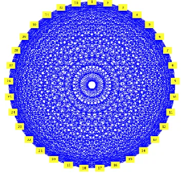
Fig. 1 The generalized commuting graph for Type 1 when     , the complete graph of 33 nodes, K₃₃. The numbered nodes represent

(5)

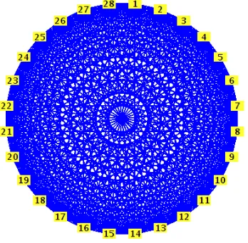
Fig. 2 The generalized commuting graph for Type 2 when ,

      the complete graph of 28 nodes, K28. The numbered nodes represent the vertices in the set



.

Fig. 3 The generalized non-commuting graph for Type 1 when ,

    an empty graph with 33 isolated vertices. The numbered nodes represent the vertices in the set



.

Fig. 4 The generalized non-commuting graph for Type 2 when ,

      an empty graph with 28 isolated vertices. The numbered nodes represent the vertices in the set



.

CONCLUSION

Throughout this research, the generalized commuting graph and generalized non-commuting graph for metacyclic 3-group for Type 1 and Type 2 have been determined. The generalized commuting graph for Type 1 has been found to be either complete with 33 vertices or null, while the generalized commuting graph for Type 2 has been found to be either complete graph with 28 vertices or null. Meanwhile, the generalized non-commuting graph for Type 1 has been found to be either 33 isolated vertices or null, while the generalized non-commuting graph for Type 2 has been found to be either 28 isolated vertices or null. It can be concluded that the graph for both type is quite similar, where they differ only in terms of the number of vertices, regardless of their presentations. The generalized commuting graph for both types are complete, whereas the non-commuting graph for both types are empty.

ACKNOWLEDGEMENT

The authors would like to acknowledge Research Management Center (RMC) Universiti Teknologi Malaysia (UTM) for the financial funding through Research University Grant (GUP) Vote No. 13H79 and Vote No. 11J96. The first author would also like to thank Ministry of Higher Education Malaysia (MOHE) for her MyPhD scholarship.

REFERENCES

Basri, A. M. A. 2013. Capability and homological functors of finite metacyclic p-groups. Doctor Philosophy, Universiti Teknologi Malaysia.

Rotman, J. J. 2002. Advanced modern algebra. (1st_{Edition). Upper Saddle River,}

N.J.: Prentice Hall.

Omer, S. M. S., Sarmin, N. H., Erfanian, A., Moradipour, K. 2013. The probability that an element of a group fixes a set and and the group act on a set by conjugation. International Journal of Applied Mathematics and Statistics. 32(2), 111-117.

Goodman, F. M. 1998. Algebra: Abstract and Concrete. Upper Saddle River, N.J.: Prentice Hall.