Analyzing and Characterizing Space and Time Sharing of the Cache Memory

ABSTRACT

KIM, SEONG BEOM. Analyzing and Characterizing Space and Time Sharing of the Cache Memory. (Under the direction of Dr. Yan Solihin.)

The dissertation studies the concurrent space sharing of the cache memory, focusing on the fairness between threads in a chip-multiprocessor (CMP) architecture. Prior work in CMP architectures has only studied throughput optimization techniques. The issue of fairness, and its relation to throughput, has not been studied.

This work makes several contributions. First, it proposes and evaluates five cache fairness metrics that measure the degree of fairness in cache sharing. Secondly, this work proposes static and dynamic L2 cache partitioning algorithms that optimize fairness. The dynamic partitioning algorithm is easy to implement, requires little or no profiling, has low overhead, and does not restrict the cache replacement algorithm to LRU. Finally, this work studies the relationship between fairness and throughput in detail. We found that optimizing fairness usually increases throughput, while maximizing throughput does not necessarily improve fairness. On average our algorithms improve fairness by a factor of 4×, while increasing the throughput by 15%, compared to a non-partitioned shared cache.

We found that each OS service exhibits multiple but limited behavior points that are re-peated frequently. In our technique, a simulation run is divided into two non-overlapping periods: alearning periodin which performance behavior of instances of an OS service are characterized and recorded, and aprediction periodin which detailed simulation is replaced with a much faster emulation.

ANALYZING AND CHARACTERIZING SPACE AND TIME

SHARING OF THE CACHE MEMORY

by

SEONG BEOM KIM

A dissertation submitted to the Graduate Faculty of

North Carolina State University

in partial fulfillment of the

requirements for the Degree of

Doctor of Philosophy

COMPUTER ENGINEERING

Raleigh, North Carolina

2007

APPROVED BY:

Dr. Edward Gehringer

Dr. Suleyman Sair

Dr. Vincent Freeh

Dr. Yan Solihin

To my beloved wife, Yoojin,

and my parents

BIOGRAPHY

Seongbeom Kim was born in Seoul, South Korea in 1972. He received BS degree in Control and Instrumentation Engineering from Seoul National University, South Korea, in 1995, and MS degree in Control and Instrumentation Engineering from the same institute, in 1997. From 1997 to 2003, Seongbeom actively participated in various research and de-velopment projects in Daewoo Electronics and Marusys. He mainly worked as a system programmer on many embedded systems including Internet Set-top Box (STB) and Digital TV STB. He has been a PhD candidate at North Carolina State University since 2003. Dur-ing the summer of 2005, Seongbeom was on an internship with the Many-Core Execution Engine team at Intel, OR.

ACKNOWLEDGMENTS

First of all, I would like to express the deepest gratitude to my adviser, Dr. Yan Solihin for his constant support, mentoring, and friendship throughout the entire duration of my PhD study. It has been challenging but fulfilling to meet his high standards toward not just the research itself but the attitude as a genuine researcher. I am thankful to Dr. William Cohen and Dr. Ravi Iyer and also to my committee members, Dr. Vincent Freeh, Dr. Edward Gehringer, and Dr. Suleyman Sair for their insightful comments and suggestions.

Warm thanks go to Dr. Mazen Kharbutli, Dhruba Chandra, Fei Guo, Brian Rogers, Rithin Shetty, Xiaowei Jiang, Christopher Hazard, Fang Liu, Aziz Eker, Abhik Sarkar, Sid-dhartha Chhabra, and Ganghee Jang, my fellow ARPERS members for their friendship and helpful comments. I am grateful to have a chance to share a part of my life with them. I specially thank Fang for her contribution to this work.

I am thankful to my parents for their love and devotion. I appreciate their lessons about being conscientious, sincere, and diligent which I will be never forget. I also ap-preciate their complete confidence in me from which I gained great strength. Finally, this dissertation would not be possible without my lovely wife, Yoojin. She has been always with me through all the moments of joy and frustration. I appreciate her prayers for me and I believe those prayers have made me what I become.

Contents

List of Tables ix

List of Figures x

1 Introduction 1

1.1 Problem Statement . . . 1

1.2 Fairness in Space-Shared Cache . . . 4

1.3 Affordable Simulation in Time-Shared Cache . . . 6

1.4 Goals and Contribution . . . 11

1.4.1 Fair Caching in a Space-Shared Cache . . . 11

1.4.2 Accelerating Full-System Simulation. . . 12

1.5 Organization of the Dissertation . . . 14

2 Fair Caching in a Space Shared Cache Memory 15 2.1 Fairness in Cache Sharing . . . 15

2.1.2 Conditions for Unfair Cache Sharing. . . 18

2.1.3 Defining and Measuring Fairness. . . 20

2.2 Cache Partitioning . . . 23

2.2.1 Hardware Support for Partitionable Caches. . . 24

2.2.2 Static Fair Caching . . . 26

2.2.3 Dynamic Fair Caching . . . 27

2.2.4 Dynamic Algorithm Overhead . . . 30

2.3 Evaluation Setup . . . 31

2.4 Evaluation . . . 34

2.4.1 Metric Correlation . . . 34

2.4.2 Static Fair Caching Results . . . 36

2.4.3 Dynamic Fair Caching Results . . . 38

2.4.4 Parameter Sensitivity. . . 42

2.5 Related Work . . . 44

3 Characterization and Analysis of Time Shared Cache Memory 47 3.1 Related Work . . . 47

3.2 Characterizing the Performance of OS Services . . . 50

3.3 Acceleration of Full-System Simulation . . . 57

3.3.2 Deriving Performance Behavior Signatures . . . 59

3.3.3 Initial Learning Mechanism . . . 62

3.3.4 Re-Learning Mechanisms . . . 64

3.3.5 Performance Prediction Mechanism . . . 69

3.4 Estimating the Performance Impact of OS Services . . . 70

3.4.1 Cache Interference Mechanism . . . 71

3.4.2 Models of OS Cache Interference . . . 73

3.5 Evaluation Environment . . . 87

3.5.1 Simulation Environment. . . 87

3.5.2 Benchmarks . . . 88

3.6 Evaluation . . . 90

3.6.1 Performance Estimation Accuracy . . . 90

3.6.2 Comparison of Re-learning Strategies . . . 94

3.6.3 Impact of Estimating OS Services Cache Interference . . . 96

3.6.4 Sensitivity Study . . . 97

3.6.5 Estimated Speedup . . . 98

3.6.6 OS Portion on a Real System . . . 99

4.2 Accelerating Full-System Simulation . . . 104

List of Tables

2.1 The applications used in our evaluation. . . 32

2.2 Parameters of the simulated architecture. Latencies correspond to contention-free conditions.RTstands for round-tripfrom the processor. . . 33

2.3 Dynamic partitioning algorithm parameters. . . 33

3.1 The slowdown ratios of various modes of simulation in Simics compared to the fastest mode: in-order processor without caches. . . 98

3.2 Estimated simulation speedup ratios. . . 99

List of Figures

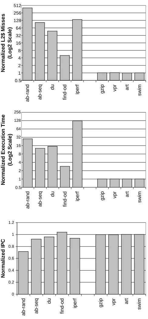
1.1 The L2 cache misses, execution time, and IPC of simulating application programs and OS, normalized to those obtained from simulating just the applications. The description of each benchmark and evaluation parameters are given in more detail in Section 3.5. . . 8

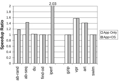
1.2 Speedup ratios obtained using a 1MB L2 cache over using a 512KB L2 cache, using application-only simulations versus using full-system simulations. . . 10

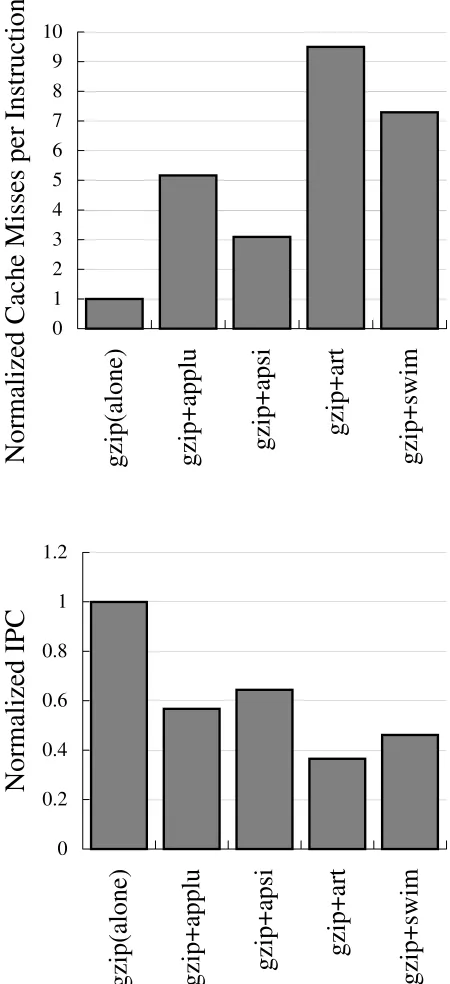
2.1 gzip’s number of cache misses per instruction and instructions per cycle (IPC), when it runs alone compared to when it is co-scheduled with another thread on a 2-processor CMP, sharing an 8-way associative 512KB L2 cache. . . 17

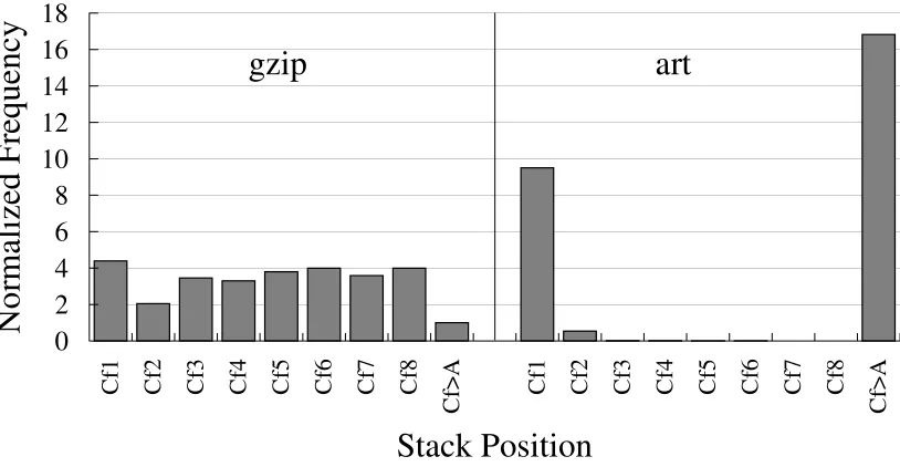
2.2 Stack distance frequency profile of gzip and art on an 8-way associative 512KB cache, collected by runninggzipandart alone. The bars are normalized togzip’s cache miss frequency (Cf>Abar). . . 20

2.3 Correlation of five L2 cache fairness metrics (M1, M2, . . . , M5) with the execution time fairness metric (M0). . . 35

2.4 Throughput (top chart) and fairness metricM1(bottom chart) of static partitioning algorithms. LowerM1values indicate better fairness. . . 36

2.5 Throughput (top chart) and fairness metricM1 (bottom chart) of dynamic

parti-tioning algorithms. LowerM1values indicate better fairness. . . 38

2.6 The distribution of partitions forFairM1Dyn. . . 40

2.7 The impact of rollback threshold (Trollback) on throughput (top chart) and fairness

2.8 The impact of repartitioning interval on throughput (top chart) and fairness metric

M1(bottom chart). LowerM1values indicate better fairness. . . 43

2.9 The impact of the partition granularity on throughput (top chart) and fairness met-ricM1(bottom chart). LowerM1values indicate better fairness. . . 44

3.1 The average and range (= average±standard deviation) of the number of simu-lated cycles (a) and IPC (b) for different OS services, forab-randandab-seq bench-marks (Section 3.5). Only OS services that are invoked more than once are shown. The IPC is computed as the number of x86 instructions committed per cycle. . . . 52

3.2 The execution time of sys read system call at different invocations for bench-marksab-rand(a), andab-seq(b). . . 55

3.3 The bubble histogram of different behavior points ofsys readforab-rand(a), and

ab-seq(b). The area of a bubble is proportional to the number of occurrences that falls into the instruction and cycle bins located at the bubble’s center. . . 58

3.4 Coefficient of variation (CV) of execution time (a) and IPC (b), when all points from each OS service are considered as a single cluster (first bar for each benchmark) versus when they are grouped intoscaled clusters(b). . . 61

3.5 The initial learning window (number of required trials) needed in order to capture all clusters of which their probabilities of occurrences are equal to or higher than the minimum probability of occurrence, given 95% or 99% degrees of confidence. . 65

3.6 The breakdown of the timeline of OS interference over application performance. . 75

3.7 The Markov Chain showing the transition from the current state(p, n)to one of three new states, when a new cache access is added. . . 77

3.8 Illustration of the relationship between the state transition probabilities and the stack distance profile for a 4-way set associative cache. . . 79

3.9 The number of additional L2 cache misses due to thereplacementand thereorder ef-fects by OS services (a), and the relative contribution of each effect to the additional L2 cache misses (b). . . 84

3.11 The miss rates for L1 instruction cache, L1 data cache, and L2 unified cache ob-tained through system simulation versus predicted by our accelerated full-system simulation scheme. . . 92

3.12 Speedup ratios obtained using a 1MB L2 cache over using a 512KB L2 cache, us-ing application-only simulations, system simulations, and our accelerated full-system simulation. . . 93

3.13 The coverage (a) and the accuracy (b) of different re-learning strategies. . . 95

3.14 The absolute prediction error for execution time, when the OS cache interference is ignored (while bar), and the interference is estimated (gray bar). . . 96

Chapter 1

Introduction

1.1. Problem Statement

During the past decades, the performance of microprocessors has improved signifi-cantly due to innovations in the architecture as well as improvement in the fabrication process. Deeply pipelined and wide-issue superscalar processors have successfully ex-ploited instruction-level parallelism in a program and improved its performance.

processors and the memory is widening. This means the cost of a cache miss in the lowest-level cache becomes more and more expensive because it involves accessing the memory. Even very aggressive superscalar processors would suffer from a long stall when there are lowest-level cache misses. Therefore, understanding the performance of the lowest-level cache is important now and likely to remain so in the future.

Secondly, complex processors would consume much power and correspondingly gen-erate so much heat such that the performance improvement often becomes less appealing. To address this problem, the current trend is to have multiple simpler cores on a chip in a Chip Multi-Processor (CMP) architecture, instead of having a single complex core [21,40]. Although this would solve the aforementioned problems, CMP architectures raise new challenges to the lowest-level cache performance because the lowest-level caches are often shared by multiple cores in CMP. We refer to this problem as the space-sharing of a cache resource. In this dissertation, we found that the space-sharing of the lowest-level cache in a CMP architecture can be very unfair and the performance implication of such unfairness can be quite significant. We address the problem of unfair space-sharing of the lowest-level cache (L2) in a dual core CMP architecture.

Considering the importance of such workloads, understanding the time-sharing aspect of cache resources is very important. Note that this problem is not specific to servers. In desktop PCs, we have more and more background processes that share cache resources in a time-multiplexed manner.

characterized and predicted. To isolate the time-shared impact, we evaluate a single core architecture so that there is no space-sharing.

1.2. Fairness in Space-Shared Cache

In a CMP architecture, the L2 cache and its lower memory hierarchy components are typically shared by multiple processors to maximize resource utilization and avoid costly resource duplication [21]. Unfortunately, cache contention due to cache sharing between multiple threads that are co-scheduled on different CMP processors can adversely im-pact throughput and fairness. Throughput measures the combined progress rate of all the co-scheduled threads, whereas fairness measures how uniformly the threads are slowed down due to cache sharing.

Prior work in CMP architectures has ignored fairness and focused on studying throughput and its optimization techniques in a shared L2 cache [22, 55]. In Simultane-ous Multi-Threaded (SMT) architectures, where typically the entire cache hierarchy and many processor resources are shared, it has been observed that throughput-optimizing policies tend to favor threads that naturally have high IPC [51], hence sacrificing fairness. Some studies have proposed metrics that, if optimized, balances between throughput and fairness [34,51].

to throughput. In contrast to prior work in CMP and SMT, we pursue fairness as the main (and separate) optimization goal. Fairness is a critical aspect to optimize because the Operating System (OS) thread scheduler’s effectiveness depends on the hardware to provide fairness to all co-scheduled threads. An OS enforces thread priorities by assigning timeslices, i.e., more timeslices to higher-priority threads. However, it assumes that in a given timeslice, the resource sharing uniformly impacts the rates of progress of all the co-scheduled threads. Unfortunately, we found that the assumption is often unmet because a thread’s ability to compete for cache space is determined by its temporal reuse behavior, which is often very different compared to that of other threads which are co-scheduled with it.

Unfortu-nately, despite these problems, cache implementations today are thread-blind, producing unfair cache sharing in many cases.

To avoid these problems, ideally the hardware should providefair caching, i.e. a scheme that guarantees that the impact of cache sharing is uniform for all the co-scheduled threads. With fair caching, the OS can mostly abstract away the impact of cache sharing, and ex-pect priority-based timeslice assignment to work as effectively as in a time-shared single processor system.

1.3. Affordable Simulation in Time-Shared Cache

To illustrate the necessity of full-system simulation for such applications, in Figure1.1

we show the L2 cache misses, execution time, and IPC estimates obtained from full-system simulation normalized to those obtained from simulating only the application programs. OS-intensive applications are shown on the left set of bars, which include web server ap-plications (ab-rand andab-seq), Unix tools (find-odanddu), and a network benchmarking tool (iperf). The right set of bars show some applications from SPEC2000 (gzip, vpr, art, andswim). The figure shows that while the number of L2 cache misses in SPEC2000 appli-cations are almost the same in both simulations, in OS-intensive appliappli-cations the number of L2 cache misses obtained by full-system simulation can be as high as 405×compared to that obtained by application-only simulation. The execution time estimates for OS-intensive applications obtained by application-only simulation are also highly inaccurate. The full system simulation’s execution time estimates are up to 126×higher than those obtained through application-only simulations. Finally, since OS code often exhibits very different instruction throughput (measured asinstructions per cycleor IPC), the estimated combined IPC is also very different in the two simulations.

ab -r and ab -s eq du fi nd

-od _iperf _gzip vpr art

s wim N or m a li z e d L 2$ M isses (Log 2 S ca le) 0.5 1 2 4 8 16 32 64 128 256 512 ab -r and ab -s eq du fi nd

-od _iperf _gzip vpr art

s wim N o rma li z e d E xec u tion Ti me (Log 2 S ca le) 0.5 1 2 4 8 16 32 64 128 256 0 0.2 0.4 0.6 0.8 1 1.2 ab -r and ab -s eq du fi nd

-od _iperf _gzip vpr art

s wim N or m a li z e d IPC

Figure 1.1:The L2 cache misses, execution time, and IPC of simulating application programs and OS, normalized to those obtained from simulating just the applications. The description of each

shows thespeedup ratio obtained when increasing the L2 cache size from 512KB to 1MB. Each application shows two bars: the first bar shows the speedup ratio by only simulating the applications (App Only) for both 512KB and 1MB L2 cache, while the second bar shows the speedup ratio obtained by simulating both the applications and the OS (App+OS) for both 512KB and 1MB L2 caches. The figure shows that while the speedup ratios for both simulations are similar for SPEC2000 applications, they are very different for OS-intensive applications. In fact, had one relied only on application-only simulations, he/she would have wrongly concluded that the performance benefits of 1MB L2 cache over 512KB L2 cache for the shown applications were negligible. However, the full-system simulation clearly leads to a different conclusion that using a 1MB L2 cache gives significantly better performance than using a 512KB L2 cache (up to 2.03×speedup for iperf).

0 0.2 0.4 0.6 0.8 1 1.2 1.4 1.6 1.8 2

ab

-r

and

ab

-s

eq

du

fi

nd

-od

ipe

rf

g

z

ip

v

pr

a

rt

s

wim

S

p

ee

dup

R

a

tio

App Only App+OS

2.03

Figure 1.2: Speedup ratios obtained using a 1MB L2 cache over using a 512KB L2 cache, using application-only simulations versus using full-system simulations.

1.4. Goals and Contribution

1.4.1. Fair Caching in a Space-Shared Cache

objective.

1.4.2. Accelerating Full-System Simulation

Our scheme is based on an observation that OS services such as system calls and in-terrupt handling often exhibit performance behavior repetitiveness. This repetitiveness is understandable because each type of OS service is designed to provide one specific func-tionality. However, unlike a phase which shows a single behavior point, we found that most OS services exhibit multiple behavior points, and the patterns of their occurrence are quite irregular depending on the applications and environments. This observation is due to the fact that the behavior of an OS service is not only determined by the parameters passed by the application, but also by the state of the service handler itself and by the environment.

signa-ture. Once learning is complete, future occurrences of the OS service are no longer fully simulated. Rather, they are profiled to obtain its signature. Its signature is then searched for a match against one of the clusters that were collected during learning, and its perfor-mance characteristics are predicted from its matching cluster. Since signature profiling can be performed in emulation mode, i.e., without involving processor and memory hierarchy timing models, most occurrences of OS services can be fast-forwarded in emulation mode and the full-system simulation can be greatly accelerated.

Overall, the contributions of this work are: performance characterization of OS ser-vices, a statistically-rigorous learning and re-learning strategy that captures OS service behavior through sampling only a fraction its occurrences, and performance prediction techniques for accelerating full-system simulation.

1.5. Organization of the Dissertation

The rest of the dissertation is organized as follows. Chapter 2 describes our contri-bution of fair caching in detail. The chapter discusses fairness in cache sharing in details and presents our metrics to measure fairness (Section2.1), presents fair caching algorithms (Section2.2), describes the evaluation environment for fair caching (Section2.3), presents and discusses the evaluation results (Section2.4), and describes related work (Section2.5).

Chapter3describes our novel simulation methodology to accelerate full-system simu-lation. It describes related work (Section3.1), presents our contribution on characterizing performance behavior of OS services (Section3.2), presents our learning strategy and per-formance prediction schemes (Section3.3), presents the methods of approximating cache interference by OS services (Section3.4), describes the evaluation environment (Section3.5) and presents validation and evaluation results (Section3.6).

Chapter 2

Fair Caching in a Space Shared Cache

Memory

2.1. Fairness in Cache Sharing

cache sharing (Section2.1.1), the conditions in which unfair cache sharing may occur (Sec-tion2.1.2), and formally defines fairness and proposes metrics to measure it (Section2.1.3).

2.1.1. Impact of Unfair Cache Sharing

To illustrate the impact of cache sharing, Figure 2.1 shows gzip’s number of cache misses per instruction and instructions per cycle (IPC), when it runs alone compared to when it is co-scheduled with different threads, such asapplu,apsi, art, andswim. All the bars are normalized to the case wheregzipis running alone. The figure shows thatgzip’s number of cache misses per instruction increases significantly compared to when it runs alone. Furthermore, the increase is very dependent on the application that is co-scheduled with it. For example, whilegzip’s cache miss per instruction increases by only3×when it runs withapsi, it increases by9.5×when it runs withartand7.3×when it runs withswim. As a result, the IPC is affected differently. It is reduced by 35% whengzipruns withapsi, but reduced by 63% whengzipruns withart. Although not shown in the figure,art,apsi, applu, andswim’s cache miss per instruction increases less than 15% when each of them runs withgzip. This creates a very unfair cache-sharing situation.

0 1 2 3 4 5 6 7 8 9 10

gz

ip

(a

lo

ne

)

gz

ip

+a

pp

lu

gz

ip

+a

ps

i

gz

ip

+a

rt

gz

ip

+s

w

im

N

or

m

al

iz

ed

C

ac

he

M

is

se

s p

er

In

st

ru

ct

io

n

gz

ip

(a

lo

ne

)

gz

ip

+a

pp

lu

gz

ip

+a

ps

i

gz

ip

+a

rt

gz

ip

+s

w

im

N

or

m

al

iz

ed

IP

C

gzip may appear to be starved. In terms of throughput, gzip’s significant slowdown re-duces the overall throughput because the utilization of the processor wheregzipruns on is also significantly reduced. Therefore, improving fairness in cache sharing is likely to also improve the overall throughput of the system.

Finally, fair caching alone cannot always prevent cache thrashing. Fair caching merely equalizes the impact of cache sharing to all the threads. However, it is still possible that the co-scheduled threads’ working sets severely overflow the cache and create a thrashing condition. Therefore, although the hardware should provide fair caching, the OS thread scheduler still needs a tool that can help it to judiciously avoid co-schedules that cause cache thrashing.

2.1.2. Conditions for Unfair Cache Sharing

To illustrate why some threads such asgzipare prone to suffer from a large increase in the number of cache misses, it is important to analyze temporal reuse behavior, obtained by stack-distance profiling1[12,31,36,55].

Stack Distance Profiling. For an A-way associative cache with LRU replacement

al-gorithm, there areA+ 1counters: C1, C2, . . . , CA, C>A. On each cache access, one of the counters is incremented. If it is a cache access to a line in theithposition in the LRU stack of the set,Ciis incremented. Note that our first line in the stack is the most recently used

line in the set, and the last line in the stack is the least recently used line. If it is a cache miss, the line is not found in the LRU stack, resulting in incrementing the miss counter

C>A. Stack distance profile can easily be obtained statically by the compiler [12], by

simu-lation, or by running the thread alone in the system [55]. It is well known that the number of cache misses for a less associative cache can be easily computed using the stack distance profile. For example, for a smaller cache that hasA0 associativity, whereA0 < A, the new number of misses can be computed as:

miss=C>A+

A

X

i=A0₊₁

Ci (2.1)

For our purposes, since we need to compare stack distance profiles from different appli-cations, it is useful to take the counter’s frequency by dividing each of the counter values by the number of processor cycles over which the profile is collected (i.e.,Cfi= _{CP U cycle}Ci ). Furthermore, we callCf>A themiss frequency, denoting the frequency of cache misses in CPU cycles. We also call the sum of all other counters, i.e.PA

i=1Cfi, thereuse frequency.

0

2

4

6

8

10

12

14

16

18

f1 _Cf2 _Cf3 _Cf4 _Cf5 _Cf6 _Cf7 _Cf8

C

f>

A

C

f1 _Cf2 _Cf3 _Cf4 _Cf5 _Cf6 _Cf7 _Cf8

C f> A

Stack Position

N

or

m

al

iz

ed

F

re

qu

en

cy

gzip

art

Figure 2.2:Stack distance frequency profile ofgzipandarton an 8-way associative 512KB

cache, collected by runninggzipandartalone. The bars are normalized togzip’s cache

miss frequency (Cf>Abar).

2.1.3. Defining and Measuring Fairness

To measure fairness, let us first define it. LetT dedidenote the execution time of thread iwhen it runs alone with a dedicated cache, and T shri denote its execution time when it shares the cache with other threads. When there are nthreads sharing the cache and assuming that the threads are always co-scheduled during their lifetime, an ideal fairness is achieved when:

T shr1

T ded1

= T shr2 T ded2

=. . .= T shrn T dedn

(2.2)

which we refer to as theexecution time fairnesscriterion. The criterion can be met if, for any pair of threadsiandjthat are co-scheduled, the following metric (M₀ij) is minimized:

M₀ij =|Xi−Xj|, whereXi= T shri T dedi

Obviously, it is difficult to measure T shri in reality because of the lack of reference points in the execution where the execution time of the shared and dedicated cache cases can be collected and compared. To enforce fairness, a metric that is easier to measure, and one that highly correlates withM0, is needed. Since we deal with an L2 cache sharing

pol-icy, the metric should only be impacted by and dependent on the L2 cache sharing polpol-icy, so that it can be reliably used as an input to the fair cache sharing algorithms. For example, instructions per cycle (IPC) is not a good metric for measuring L2 cache sharing fairness because it is highly dependent on many external factors, such as the available ILP, different types of processor hazards, branch mispredictions, L1 data and instruction caches, TLBs, etc. How responsive the IPC is to the L2 cache sharing policy is very application-specific, can have a large range of values, and is therefore unreliable. In addition, IPC is prone to change in response to power-saving techniques, such as frequency and voltage scaling, fetch gating, etc.

We propose five L2 cache-fairness metrics that are directly related to the L2 cache per-formance and are insensitive to external factors, while at the same time easy to measure. Let M issandM issr denote the number of misses and miss rates, respectively. For any pair of co-scheduled threadsiandj, the following metrics measure the degree of fairness between a thread pair:

M₁ij = |Xi−Xj|, whereXi=

M iss shri M iss dedi

(2.4)

M₂ij = |Xi−Xj|, whereXi=M iss shri (2.5)

M₃ij = |Xi−Xj|, whereXi=

M issr shri M issr dedi

M₄ij = |Xi−Xj|, whereXi=M issr shri (2.7)

M₅ij = |Xi−Xj|, where

Xi=M issr shri−M issr dedi (2.8)

By minimizingMij

x , a fair caching algorithm seeks to improve fairness. When there are more than two threads, the fairness metrics can be summed or averaged over all possible pairs, and the resulting metric, e.g.Mx =Pi

P

jMxij, becomes the target for minimization. Metric M1 tries to equalize the ratio of miss increase of each thread, while M2 tries to

equalize the number of misses. Similarly, metricM3tries to equalize the ratio of miss rate

increase of each thread, whileM4 tries to equalize the miss rates. Finally, metricM5 tries

to equalize the increase in the miss rates of each thread.

MetricsM2 andM4 enforce fairness in absolute terms, that is, the number of misses,

or the miss rates under sharing are equalized. They may over-penalize applications with few misses or low miss rates. In M1 andM3, the number of misses and miss rates are

normalized by those from a dedicated L2 cache, so that the increase of misses or miss rates is proportional to ones from the dedicated cache case. The normalization makes sense because, when an application suffers many misses (or has high miss rates), it is likely that many of these misses are overlapped with each other. Therefore, an increase has a smaller impact on the execution time of the application, compared to applications with few misses or low miss rates. Finally, the metricM5 adjusts the miss rates by subtracting from them

the miss rates on the dedicated cache. At this point, it seems that M1, M3, and M5 are

cache case.

The remaining issue for the metrics is how well they correlate with the execution time fairness metricM0 (Equation2.3). To find out, we compute the statistical correlation [16]

betweenM0andMi, wherei= 1,2, . . . ,5:

Corr(Mi, M0) =

Cov(Mi, M0)

σ(Mi)σ(M0)

,where (2.9)

Cov(Mi, M0) = E(MiM0)−E(Mi)E(M0)

whereσ(Mi) andE(Mi) denote the standard deviation and expected value ofMi. Since we are interested in how the L2 cache sharing policy impacts both the execution time fairness metric (M0) and other fairness metrics (Mi), we can obtain one data point for each L2 sharing policy. For example, by partitioning the L2 cache atndifferent partition sizes, we obtainndata points, which can be used to computeCorr(Mi, M0). The value of

Corr(Mi, M0)ranges from−1to 1, where 1 indicates a perfect correlation, 0 indicates no

correlation, and−1indicates negative correlation. A perfect correlation betweenMi and M0indicates thatMican be used in place ofM0to guide a fair caching policy.

2.2. Cache Partitioning

In Section2.2.1, we adapt themodified LRUhardware support for partitionable caches from Suh, et al. [55]. Although we use similar hardware support, our partitioning algo-rithms (Section2.2.2and 2.2.3) are different in that while they optimize throughput, we optimize fairness. In addition, while their dynamic partitioning algorithms rely on the cache to implement true LRU replacement algorithm, our dynamic partitioning algorithms can work with any replacement algorithms. This is important because the L2 cache often implements pseudo-LRU replacement algorithms (such as Cvetanovic’s [14]), partly due to the complexity of implementing LRU replacement for highly associative caches, and partly due to a small performance difference between LRU and random replacement in large and highly associative caches [19]. Therefore, to be useful, a cache partitioning algo-rithm should work with pseudo-LRU replacement algoalgo-rithms.

2.2.1. Hardware Support for Partitionable Caches

In general, hardware support for partitionable caches can be categorized into two ap-proaches. The first approach relies on modifying the cache placement algorithm by restrict-ing where data can be placed in the cache [22, 45]. This approach relies on configurable cache hardware or programmable partition registers. The drawbacks of this approach are that it modifies the underlying cache hardware, may increase the cache access time due to having to locate the correct partition, and makes the cache unavailable during reconfigu-ration.

approach, partitioning the cache is incremental: on each cache miss, we can reallocate a cache line from another thread to the thread that suffers the cache miss by selecting the line for replacement. Because a replacement only occurs on cache misses, this approach does not add to cache access time. In addition, selecting a line to be replaced can be over-lapped with the cache miss latency. Finally, due to the incremental repartitioning nature, the repartitioning does not make the cache unavailable. It involves writing to a counter the target number of lines and tracking the current number of lines already allocated to a thread. In this work, we apply the alternative approach.

same as the thread’s target allocation. Programming a new partition is accomplished by writing to the target allocation register of each thread.

One parameter of the cache is the partition granularity, the smallest unit of partition that can be reallocated. Ideally, taking into account the number of cores, it should be as coarse-grained as possible without sacrificing the ability to enforce fairness. For 2-way CMP, we found that a partition granularity equal to the total cache space divided by its as-sociativity, works well. For example, for an 8-way 512KB L2 cache, the granularity would be 64KB.

2.2.2. Static Fair Caching

Our static fair caching algorithm partitions the cache based on the stack distance profile of an application, collected through a profiling run. The stack distance profile can only be collected when the cache uses an LRU replacement algorithm, or at least records the LRU stack information. Note that we only need to perform one profiling run per application.

For static partitioning, we first run each application and collect its global stack distance frequency profile described in Section2.1.2. LetP =< p1, p2, . . . , pn >,Ppi =cacheSize, denote a partition. Then, for each thread iand partition P, we apply Equation 2.1, us-ing A0 = pi

numSet×lineSize to obtain the expected new misses (M iss shri) and miss rate

because the thread mix may have changed.

The benefit of static partitioning is that it can be used as an input to the OS thread scheduler to avoid co-scheduling threads that will cause cache thrashing. As discussed in Section2.1.1, cache partitioning alone cannot prevent all cases of cache thrashing. The drawback is that static partitioning relies on the cache to implement LRU replacement algorithm and is unable to adapt to applications’ dynamic behavior.

2.2.3. Dynamic Fair Caching

However, since the cache never becomes unavailable when the algorithm is invoked, the algorithm latency is not much of a critical issue.

Initialization.

Initialize partition equally, pi = cacheSize_n , wherenis the number of cores or threads sharing the cache. Apply that for the first interval period.

In the rollback step, the considered set is initialized to contain all the co-scheduled threads, indicating that by default all of them will be considered for repartitioning (Step 1). Then each threadiis checked whether it has received a larger partition in the time interval that just completed (t), indicated by a repartitioning assignmentAij being a member of the repartition assignment setAS, which was recorded in the prior time interval by the repar-titioning step. For such a thread, if its new miss rate has not decreased by at leastTrollback, the prior repartitioning assignment is deemed ineffective, and therefore it is rolled back to what it was before that (Step 2). In addition, both threads iandj are removed from the considered set, so that they will no longer be considered by the repartitioning step.

Rollback Step. At the end of an interval periodt:

1. Initialize Considered SetCS ={1,2, . . . , n}.

2. For each threadi,ifa repartition assignmentAij ∈AS, whereAS is the repar-tition assignment set,andM issr shrt_i−1−M issr shrt_i ≤Trollback, roll back the repartitioning assignment:

• pt_i+1=pt_i−1

• pt_j+1=pt_j−1

Repartitioning Step. At the end of an interval periodt, and right after the rollback step:

1. Initialize repartition assignmentAS ={}.

2. For each threadi∈CS, compute the statistics related to the fairness metric being optimized. For example, for metricM1, we computeXit=

M iss shri

M iss dedi, whereas for

M3, we computeXit=

M issr shri

M issr dedi.

3. Findimax ∈ CS andimin ∈ CS such thatXimax andXimin have the maximum and minimum values, respectively.

4. IfXimax−Ximin> Trepartition≥0then reassign the partition: • pt_i+1_max =pt_imax+gran

• pt_i+1 min=p

t

imin−gran

• AS =ASS{A

imaximin}

5. CS=CS− {imax, imin}.

6. Repeat step 2 to 5 untilCS ={}.

7. Apply the partition in the next interval periodt+ 1.

The parameters for the algorithms are the partition granularity (gran), rollback thresh-old (Trollback), repartitioning threshold (Trepartition), and the time interval period.

2.2.4. Dynamic Algorithm Overhead

There are three types of overheads in our dynamic partitioning schemes: profiling overhead, storage overhead, and fair caching algorithm overhead. A single static profil-ing run per thread is needed to obtain the base miss per cycle (representprofil-ing miss count) and miss rate, except when the algorithm optimizes theM2 orM4 metrics, in which case

overhead, we need a few registers per thread to keep track of the miss count or miss rate of the current and prior time intervals. Finally, we assume that the fair caching algorithm is implemented in hardware, and therefore does not incur any algorithm overhead. How-ever, we have also measured the overhead of a software implementation of the algorithm for a 2-processor CMP and found that the algorithm takes less than 100 cycles to run per invocation, making a software implementation a feasible alternative. Furthermore, since the algorithm invocation does not make the cache unavailable and can be overlapped with the application execution, its latency can be hidden. Even when compared to the smallest time interval, the overhead is less than 0.01%.

2.3. Evaluation Setup

Applications. To evaluate the benefit of the cache partitioning schemes, we choose a set

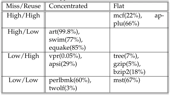
of mostly memory-intensive benchmarks: apsi, art,applu, bzip2, equake,gzip, mcf,perlbmk, swim,twolf, andvprfrom the SPEC2000 CPU benchmark suite [53];mstfrom Olden bench-mark, andtree[9]. We used test input sets for the SPEC2000 CPU benchmarks, 1024 nodes for mst, and 2048 bodies for tree. Most benchmarks are simulated from start to completion, with an average of 786 millions instructions simulated.

Table 2.1:The applications used in our evaluation. Miss/Reuse Concentrated Flat

High/High mcf(22%),

ap-plu(66%) High/Low art(99.8%),

swim(77%), equake(85%) Low/High vpr(0.05%),

apsi(29%)

tree(7%), gzip(5%), bzip2(18%) Low/Low perlbmk(60%),

twolf(3%)

mst(67%)

1000 CPU cycles are more than 2. It is categorized into the “Flat” category if the standard deviation of its global stack distance frequency counters is smaller than 0.1. Otherwise, it is categorized into “Concentrated”. Finally, all data is collected for the benchmark’s entire execution time, which may differ from when they are co-scheduled. The table shows that we have a wide range of benchmark behavior. These benchmarks are paired and co-scheduled. Eighteen benchmark pairs are co-scheduled to run on separate CMP cores that share the L2 cache. To observe the impact of L2 cache sharing, each benchmark pair is run from the start and is terminated once one of the benchmarks completes execution.

Simulation Environment. The evaluation is performed using a cycle-accurate,

replace-ment.

Table 2.2:Parameters of the simulated architecture. Latencies correspond to

contention-free conditions.RTstands for round-tripfrom the processor.

CMP

2 cores, each 4-issue out-of-order, 3.2 GHz Int, fp, ld/st FUs: 2, 2, 2

Max ld, st: 64, 48. Branch penalty: 17 cycles Re-order buffer size: 192

MEMORY

L1 Inst (private): WB, 32KB, 4 way, 64-B line, RT: 3 cycles L1 data (private): WB, 32KB, 4 way, 64-B line, RT: 3 cycles L2 data (shared): WB, 512KB, 8 way, 64-B line, RT: 14 cycles L2 replacement: LRU or pseudo-LRU

RT memory latency: 407 cycles

Memory bus: split-transaction, 8 B, 800 MHz, 6.4 GB/sec peak

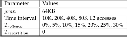
Algorithm Parameters. The parameters for the fair caching algorithm discussed in

Sec-tion2.2.3are shown in Table2.3. The time interval determines how many L2 cache accesses must occur before the algorithm is invoked. We also vary the rollback threshold (Trollback), while the repartition threshold (Trepartition) is set to 0. Although the partition granular-ity can be any multiples of a cache line size, we choose 64KB granulargranular-ity to balance the speed of the algorithm in achieving the optimal partition, and the ability of the algorithm to approximate an ideal fairness.

Table 2.3:Dynamic partitioning algorithm parameters. Parameter Values

gran 64KB

Time interval 10K, 20K, 40K, 80K L2 accesses

Trollback 0%, 5%, 10%, 15%, 20%, 25%, 30%

Dedicated Cache Profiling. Benchmark pairs are run in a co-schedule until a thread that is

shorter completes. At that point, the simulation is stopped to make sure that the statistics collected reflect the impact of L2 cache sharing. To obtain accurate dedicated mode pro-files, the profile duration should correspond to the duration of the co-schedules. For the shorter thread, the profile is collected for its entire execution in a dedicated cache mode. But for the longer thread, the profile is collected until the number of instructions executed reaches the number of instructions executed in the co-schedule.

2.4. Evaluation

In this section, we present and discuss several sets of evaluation results. Section2.4.1

presents the correlation of the various fairness metrics. Section2.4.2discusses the results for the static partitioning algorithm, while Section 2.4.3discusses the results for the dy-namic partitioning algorithm. Finally, Section 2.4.4discusses how sensitive the dynamic partitioning algorithm is to its parameters.

2.4.1. Metric Correlation

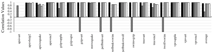
Figure2.3presents the correlation of L2 cache fairness metrics (M1, M2, . . . , M5) with

the execution time fairness metric from Equation 2.3 (M0). We collect one data point of

-1 -0.8 -0.6 -0.4 -0.20 0.2 0.4 0.6 0.81 ap si +a rt ap si +b zi p2 ap si+ eq ua ke ap si +m cf gz ip +a pp lu gz ip +a ps i gz ip +a rt m st +e qu ak e pe rlb m k+ ar t pe rlb m k+ sw im pe rlb m k+ tw ol f sw im +g zi p tre e+ ar t tre e+ m cf tw ol f+ sw im vp r+ ap pl u vp r+ ar t vp r+ m cf av er ag e C or re la tio n V al ue s

Corr(M1,M0) Corr(M2,M0) Corr(M3,M0) Corr(M4,M0) Corr(M5,M0)

Figure 2.3:Correlation of five L2 cache fairness metrics (M1, M2, . . . , M5) with the execution time

fairness metric (M0).

The figure shows that on average,M1,M3,M4andM5produce good correlation (94%,

92%, 91%, and 92%, respectively), whereasM2 produces poor correlation (37%). It is clear

thatM1is the best fairness metric, not only on average, but also across all the benchmark

pairs. The second best metric is M3 where it consistently has a high correlation on all

benchmark pairs. Therefore, for the rest of the evaluation, we only considerM1 andM3

for our fairness metrics.

M4 andM5 occasionally do not correlate as well as M3, such as for benchmark pairs

apsi+equakeandtree+mcf. Zero correlation appears inapsi+artfor most metrics, showing an anomaly caused by constant values of the metrics regardless of the partition sizes, versus the M0 metric which produces a very slight change due to external factors such as bus

contention. In five benchmark pairs,M2 produces negative correlation, indicating that it

is not a good metric to use for measuring fairness. This is because equalizing the number of misses over-penalizes threads that originally have few misses. Therefore, enforcingM2

Note that most of the benchmarks tested are L2 cache intensive, in that they access the L2 cache quite frequently. It is possible that benchmarks that do not access the L2 cache much may not obtain a high correlation between the L2 fairness metrics and the execution time fairness. However, arguably, such benchmarks do not need high correlation values because they do not need fair caching. Even when their number of L2 cache misses increases significantly, their execution time will not be affected much.

2.4.2. Static Fair Caching Results

0 0.2 0.4 0.6 0.81 1.2 1.4 1.6 1.82 ap si +a rt ap si +b zi p2 ap si +e qu ak e ap si +m cf gz ip +a pp lu gz ip +a ps i gz ip +a rt m st +e qu ak e pe rlb m k+ ar t pe rlb m k+ sw im pe rlb m k+ tw ol f sw im +g zi p tre e+ ar t tre e+ m cf tw ol f+ sw im vp r+ ap pl u vp r+ ar t vp r+ m cf av er ag e N or m al iz ed C om bi ne d IP

C _{LRU MinMiss FairM1 Opt}

0 0.2 0.4 0.6 0.81 1.2 1.4 1.6 ap si +a rt ap si +b zi p2 ap si +e qu ak e ap si +m cf gz ip +a pp lu gz ip +a ps i gz ip +a rt m st +e qu ak e pe rlb m k+ ar t pe rlb m k+ sw im pe rlb m k+ tw ol f sw im +g zi p tre e+ ar t tre e+ m cf tw ol f+ sw im vp r+ ap pl u vp r+ ar t vp r+ m cf av er ag e N or m al iz ed F ai rn es s M

1 LRU MinMiss FairM1 Opt

10.1/4.2/2.3 2.6/2.6

Figure 2.4:Throughput (top chart) and fairness metricM1(bottom chart) of static

parti-tioning algorithms. LowerM1values indicate better fairness.

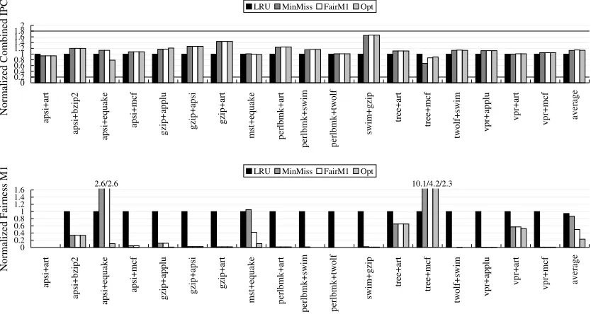
Figure 2.4 shows the throughput (combined IPC) on the top chart and M1 fairness

first bar (LRU) is a non-partitioned shared L2 cache with LRU replacement algorithm. The second bar (MinMiss) is a L2 cache partitioning scheme that minimizes the total number of misses of the benchmark pair.MinMissis similar to the scheme in [55], except thatMinMiss finds such partition statically. The third bar (FairM1) is our L2 cache partitioning algorithm that enforces fair caching by minimizing theM1 metric for each benchmark pair. The last

bar (Opt) represents the best possible (most fair) partition.Optis obtained by running the benchmark pairs once for every possible partition. The partition that produces the best fairness is chosen forOpt. All bars are normalized toLRU, except for apsi+art, in which case all schemes, includingLRU, achieve an ideal fairness. For static partitioning, to obtain precise target partitions, the same partition sizes are kept uniform across all the sets.

On average, all schemes, including MinMiss, improve the fairness and throughput compared toLRU. This indicates that LRUproduces a very unfair L2 cache sharing, re-sulting in poor throughput because in many cases one of the co-scheduled threads is sig-nificantly slowed down compared to when it runs alone.MinMissincreases the combined IPC by 13%. However, it fails to improve the fairness much compared toLRU, indicating that maximizing throughput does not necessarily improve fairness.

FairM1 achieves much better fairness compared to both LRU and MinMiss, reduc-ing theM1 metric by 47% and 43% compared to LRU andMinMiss, respectively.

impact of cache sharing on all threads, it avoids the pathological throughput where one thread is starved and its IPC is significantly penalized. The exceptional cases areapsi+art, apsi+equake, and tree+mcf, where evenOpt yields a lower throughput compared to LRU. Out of these three cases, the throughput reduction inapsi+equakeandtree+mcfare due to the limitation of a static partition to adapt to the changing dynamic behavior of the bench-mark pairs. They are much improved by the dynamic fair caching algorithms.

2.4.3. Dynamic Fair Caching Results

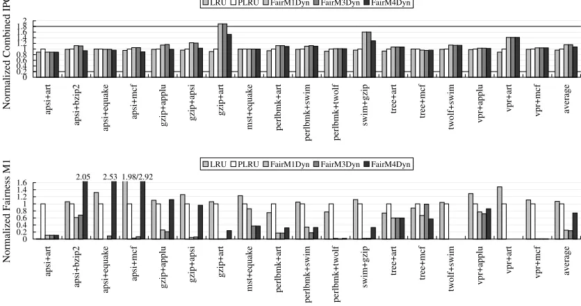
0 0.2 0.4 0.6 0.81 1.2 1.4 1.6 1.82 ap si +a rt ap si +b zi p2 ap si +e qu ak e ap si +m cf gz ip +a pp lu gz ip +a ps i gz ip +a rt m st +e qu ak e pe rlb m k+ ar t pe rlb m k+ sw im pe rlb m k+ tw ol f sw im +g zi p tre e+ ar t tre e+ m cf tw ol f+ sw im vp r+ ap pl u vp r+ ar t vp r+ m cf av er ag e N or m al iz ed C om bi ne d IP

C _{LRU PLRU FairM1Dyn FairM3Dyn FairM4Dyn}

0 0.2 0.4 0.6 0.81 1.2 1.4 1.6 ap si +a rt ap si +b zi p2 ap si +e qu ak e ap si +m cf gz ip +a pp lu gz ip +a ps i gz ip +a rt m st +e qu ak e pe rlb m k+ ar t pe rlb m k+ sw im pe rlb m k+ tw ol f sw im +g zi p tre e+ ar t tre e+ m cf tw ol f+ sw im vp r+ ap pl u vp r+ ar t vp r+ m cf av er ag e N or m al iz ed F ai rn es s M

1 LRU PLRU FairM1Dyn FairM3Dyn FairM4Dyn 2.05 2.53 1.98/2.92

Figure 2.5: Throughput (top chart) and fairness metricM1(bottom chart) of dynamic

partitioning algorithms. LowerM1values indicate better fairness.

(IPC) and metricM1, respectively. Each benchmark pair shows the result for four schemes.

The first bar (LRU) is a non-partitioned shared L2 cache with LRU replacement algorithm. The second bar (PLRU) is a non-partitioned shared L2 cache with pseudo-LRU replace-ment algorithm described in Section2.3. The last three bars (FairM1Dyn,FairM3Dyn, and FairM4Dyn) are our L2 algorithms from Section2.2.3which minimizeM1,M3, andM4

met-rics, respectively. All the bars are normalized toPLRU, which is selected as the base case because it is a more realistic L2 cache implementation, and that unlike the static algorithm, our dynamic algorithms can work with it. LRUis the same as in Figure2.4but looks dif-ferent in the chart because it is normalized toPLRU. The results in the figure are obtained using 10K L2 accesses for the time interval period, and 20% for the rollback threshold.

The figure shows that PLRU andLRU achieve roughly comparable throughput and fairness. FairM1Dyn andFairM3Dynimprove fairness over PLRUsignificantly, reducing the M1 metric by a factor of 4 on average (or 75% and 76%, respectively) compared to

PLRU. This improvement is consistent over all benchmark pairs, except for FairM3Dyn on tree+mcf. Intree+mcf, PLRUalready achieves almost ideal fairness, and therefore it is difficult to improve much over this.

throughput decrease is inapsi+art and tree+mcf, where FairM1Dynreduces the through-put by 11% and 4%, respectively. In those cases, the fairness is improved (M1 is reduced

by 89% and 33%, respectively). This implies that, in some occasions, optimizing fairness may reduce throughput.

0% 20% 40% 60% 80% 100% ap si +a rt ap si +b zi p2 ap si +e qu ak e ap si +m cf gz ip +a pp lu gz ip +a ps i gz ip +a rt m st +e qu ak e pe rlb m k+ ar t pe rlb m k+ sw im pe rlb m k+ tw ol f sw im +g zi p tre e+ ar t tre e+ m cf tw ol f+ sw im vp r+ ap pl u vp r+ ar t vp r+ m cf

Fr

eq

ue

nc

y

of

P

ar

tit

io

n

Figure 2.6:The distribution of partitions forFairM1Dyn.

Since the height of theLRUbar in the figure is almost the same as in Figure2.4(0.94 vs. 1.07), we can approximately compare how the dynamic partitioning algorithms perform with respect to the static partitioning algorithms. Comparing the two figures, it is clear that the dynamic partitioning algorithms (FairM1DynandFairM3Dyn) achieve better fairness compared to FairM1 (0.25 and 0.24 vs. 0.5) and even achieve a slightly better average throughput. This is nice because compared toFairM1, the dynamic partitioning algorithms do not require stack distance profiling or rely on an LRU replacement algorithm.

im-proves throughput by 8% and reduceM1 metric value by 26%. Although it is worse than

FairM1DynandFairM3Dyn, it may be attractive due to not requiring any profiling infor-mation. Also note thatFairM4Dyn’s pathological cases seem to be isolated to only a few benchmark pairs in which one of the threads isapsi, which suffers from a very high L2 miss rate. Therefore,FairM4Dynis a promising algorithm that needs to be investigated more thoroughly.

Figure2.6shows the fraction of all time intervals where each different partition is ap-plied, for each benchmark pair using theFairM1Dynalgorithm. An ’x-y’ partition means that the first thread is assigned x₈ ×100%of the cache, while the second thread is assigned

y

8 ×100%of the cache. To collect the data for the figure, at the end of every time interval,

we increment the partition count reflecting the partition size that was applied in the time interval just completed.

2.4.4. Parameter Sensitivity

C _{0% 5% 10% 15% 20% 25% 30%}

0 0.2 0.4 0.6 0.81 1.2 1.4 1.6 ap si +a rt ap si +b zi p2 ap si +e qu ak e ap si +m cf gz ip +a pp lu gz ip +a ps i gz ip +a rt m st +e qu ak e pe rlb m k+ ar t pe rlb m k+ sw im pe rlb m k+ tw ol f sw im +g zi p tre e+ ar t tre e+ m cf tw ol f+ sw im vp r+ ap pl u vp r+ ar t vp r+ m cf av er ag e N or m al iz ed F ai rn es s M

1 0% 5% 10% 15% 20% 25% 30%

Figure 2.7: The impact of rollback threshold (Trollback) on throughput (top chart) and

fairness metricM1(bottom chart). LowerM1values indicate better fairness.

Impact of Rollback Threshold. In the previous section, Figure2.6 highlights the im-portance of the rollback mechanism in the dynamic partitioning algorithms in rolling back from bad repartitioning decision. The rollback threshold is used by the dynamic algo-rithms to undo the prior repartition assignment if it fails to reduce the miss rate of a thread that was given a larger partition. A higher rollback threshold makes the algorithm more conservative, in that it is harder to assign a new partition (without rolling it back) unless the miss rate improvement is more substantial.

shows that the rollback threshold affects the throughput and fairness in some benchmark pairs in a very benchmark pair-specific manner. However, although theM1 metric value

changes with the threshold, the throughput improvement overPLRUdoes not vary much. Finally, on average, 20% rollback threshold achieves the best fairness.

0 0.2 0.4 0.6 0.81 1.2 1.4 1.6 1.82 ap si + art ap si + b zi p2 ap si + equ ake ap si + m cf g zi p + app lu g zi p + ap si g zi p + art m st + equ ake p erl b m k + art p erl b m k + sw im p erl b m k + tw o lf sw im + g zip tr ee + art tr ee + m cf tw o lf + sw im vp r+ app lu vp r+ art vp r+ m cf av er ag e No rma li ze d C o m bin ed

IPC 10K 20K 40K 80K

0 0.2 0.4 0.6 0.81 1.2 1.4 1.6 ap si + art ap si + b zi p2 ap si + equ ake ap si + m cf g zi p + app lu g zi p + ap si g zi p + art m st + equ ake p erl b m k + art p erl b m k + sw im p erl b m k + tw o lf sw im + g zip tr ee + art tr ee + m cf tw o lf + sw im vp r+ app lu vp r+ art vp r+ m cf av er ag e No rma li ze d Fa ir n ess

M1 10K 20K 40K 80K

Figure 2.8: The impact of repartitioning interval on throughput (top chart) and fairness

metricM1(bottom chart). LowerM1values indicate better fairness.

0 0.2 0.4 0.6 0.81 1.2 1.4 1.6 1.82 ap si + art ap si + b zi p2 ap si + equ ake ap si + m cf g zi p + app lu g zi p + ap si g zi p + art m st + equ ake p erl b m k + art p erl b m k + sw im p erl b m k + tw o lf sw im + g zip tr ee + art tr ee + m cf tw o lf + sw im vp r+ app lu vp r+ art vp r+ m cf av er ag e No rma li ze d C o m bin ed

IPC 64KB 32KB 16KB 8KB

0 0.2 0.4 0.6 0.81 1.2 1.4 1.6 ap si + art ap si + b zi p2 ap si + equ ake ap si + m cf g zi p + app lu g zi p + ap si g zi p + art m st + equ ake p erl b m k + art p erl b m k + sw im p erl b m k + tw o lf sw im + g zip tr ee + art tr ee + m cf tw o lf + sw im vp r+ app lu vp r+ art vp r+ m cf av er ag e No rma li ze d Fa ir n ess

M1 64KB 32KB 16KB 8KB

Figure 2.9:The impact of the partition granularity on throughput (top chart) and fairness

metricM1(bottom chart). LowerM1values indicate better fairness.

Impact of Partition Granularity. Figure2.9shows the throughput and fairness results with different partition granularity values ranging from 64KB to 8KB. With a large granu-larity, it takes less time to converge to an optimal partition, but if the granularity becomes too coarse, it might not exactly reach the optimal partition. With a small granularity, it takes longer time to converge to the optimal partition, but it can accurately achieve the op-timal partition. The result shows that 64KB granularity shows slightly better throughput and fairness. It means the ability of quickly reaching the target partition is more important.

2.5. Related Work

In Simultaneous Multi-Threaded (SMT) architectures, where typically the entire cache hierarchy and many processor resources are shared, metrics that mix throughput and fair-ness have been studied. The need to consider both aspects is intuitive given the large number of resources that are shared by SMT threads. Even in SMT architectures, however, the studies have only focused on either improving throughput, or improving throughput without sacrificing fairness too much [20,50,51,34]. Fairness has not been studied as the main or separate optimization goal. For example, a weighted speedup, which incorporates fairness to some extent, has been proposed by Snavely, et al. [51]. Luo, et al. proposed har-monic mean of each thread’s individual speedups to encapsulate both throughput and fair-ness [34]. Typically, to achieve the optimization goal, fetch policies, such as ICOUNT [18], can be used to control the number of instructions fetched from different SMT threads.

Chapter 3

Characterization and Analysis of

Time Shared Cache Memory

3.1. Related Work

There have been many studies that try to accelerate cycle-accurate processor simula-tions [10,11,13,26,27,29,30,33,42,43,44,46,47,48,49,58,60]. In general, the acceleration techniques can be categorized intoreduced input set,statistical simulation, andsampling-based simulation. An example of reduced input set simulations includes MinneSPEC [17], which carefully designed input sets that allow shorter simulations while still preserving the per-formance characteristics of larger input sets.

In sampling-based simulations, only samples of the dynamic instructions are simu-lated. One very simple sampling method was to skip the initialization phase of a program and simulate the next few billions of instructions. More statistically rigorous sampling methods have also been proposed. One popular class of such methods isphase-based sam-pling(e.g. SimPoint), in which a program execution is divided into intervals which exhibit uniform performance behavior calledphases. Since the program performance behavior is uniform within a single phase, a subset of instructions from that phase can be selected for simulation to represent the entire phase. Phases can be constructed from fixed-length inter-vals [10,29,42,43,44,47,48], or from intervals that correspond to natural code boundaries such as subroutines and loop structures [26,27,31,33]. Another type of sampling-based simulation approach relies on random or systematic selection of samples (e.g. SMARTS), rather than relying on phases [13,58,60]. In these studies, detailed simulation is only per-formed on samples, and it is fast-forwarded between samples. The size and quantity of samples are selected in such a way to satisfy a target degree of confidence.

While other sampling-based methods can be extended and applied to full-system simula-tion, they do not have the ability to separate the performance characteristics of OS services from one another and from the application. In contrast, our scheme is designed to provide such separation, by defining the samples at system call boundaries, and by keeping track of different types of OS services invoked by the system calls.

In addition, most of existing sampling-based simulation acceleration approaches is de-signed for accelerating application-only simulation. The performance behavior of OS ser-vices is very different from that of application programs. While an application program performance is largely only influenced by its own code characteristics, the performance of OS service is affected by four components: its owncode characteristics, theparametersit re-ceives through interacting with the application program, thestateit maintains as a result of its previous invocations, andexternal factorssuch as asynchronous events like timer and I/O interrupts, or the load of the system at the time the application runs. Consequently, acceleration approaches that require offline analysis, or samples that are determined in one run [10,13,26,27,29,33,43,44,47,48,58,60] but are applied in another run, cannot take into account the variation of OS performance on different runs, and hence are less applicable for accelerating OS-intensive applications. In contrast, in our method samples are collected, recorded, and used for prediction during live runs.

services. It is also complementary because decoupling the simulation of application code and OS services at the boundary of user/kernel mode switches makes application-only techniques more accurate, because the performance of application execution is only deter-mined by its own code and machine characteristics.

3.2. Characterizing the Performance of OS Services

This section describes this work’s contribution on characterizing the performance pat-terns of OS services and discusses the implications for designing full-system simulation acceleration techniques. First, we define anOS serviceas a specific type of system call or interrupt handling in the privileged kernel mode. We also define anOS service intervalas a contiguous group of dynamic instructions starting from when a system call or interrupt causes a mode switch to the kernel until right before it returns to the user mode. These definitions imply that all instructions executed in the non-privileged mode are considered as parts of the application code. While some instructions executed in non-privileged mode help interface with the respective OS service, such as setting up the OS stack and saving contexts, we found these instructions to be relatively few compared to the OS service code executed in the privileged mode. We also treat system libraries that are primarily imple-mented in the user mode, such as memory-allocation functions, as a part of the application. However, we note that our technique can be easily extended to cover them.

example of a synchronous OS service issys read()which is invoked when an applica-tion calls a C library funcapplica-tionfread(). Another example includes exceptions that occur due to executing instructions of the application, such as floating-point exceptions, page faults, and segmentation faults. Examples of asynchronous OS services include interrupts due to I/O availability, timer interrupts, DMA transfers, etc. Our characterization of OS services is performed on every mode switch, so it includes both synchronous and asyn-chronous OS services.

Each OS service interval defines a natural execution boundary between the application and OS services. On each mode switch, the information of the type of OS service invoked is easily available. For example, whensys enteroccurs, the type of service can be read from a register, such as the registerEAX in x86 architecture. We note that in Linux 2.6.x, there are more than 200 types of OS services defined in its system call table. Some of the OS services may overlap with others, such as when a system call handling invokes another system call of a different type. While it is possible to identify such an overlap and break an interval into smaller non-overlapping ones, we choose a simpler approach that deter-mines the type of an OS service based on the event that initially causes the transition to the privileged mode. All other OS services triggered afterward are considered as extensions of the initial OS service.

0 10000 20000 30000 40000 50000 60000 70000 sys _ c lo se sys _ fc n tl64 sys _ge tt im eo fday sys _ipc sys _open sys _poll sys _ read sys _ s o ck e tc all sys _ s ta t64 sys _w ri te sys _w ri tev In t_121 In

t_239 _Int_49

N

u

m

b

e

r

o

f

C

yc

les

t_239 _Int_49

IPC

ab-rand ab-seq

(b)

Figure 3.1: The average and range (= average±standard deviation) of the number of simulated

cycles (a) and IPC (b) for different OS services, for ab-randand ab-seqbenchmarks (Section 3.5).

its range, defined as the average plus minus its standard deviation. The white bars are for theab-randbenchmark while the gray bars are for theab-seqbenchmark. The figure shows that on average, each OS service involves a few thousands to a few tens of thousands of instructions. This observation implies that fixed-length intervals should not be used to record and characterize OS services because they would fail to correspond to the OS service boundaries. The figure also points out that the OS service intervals we choose from the natural boundary of mode switches are already veryfine-grain.

Comparing the different OS services, the figure shows that different OS services show different behavior points, characterized by unique average execution time and IPC. This observation implies that it is necessary to characterize each OS service typeseparately. An-other observation is that the average behavior is also quite different from one benchmark to another, indicating that the interaction of the applications and OS affect the performance of OS services. This implies that prediction of OS service performance cannot be based on offline analysis, and instead should be based ononline profiling. Finally, we note that the behavior variation range is very high for most OS services. This indicates that each OS service shows not one but multiple behavior points that greatly differ from one another.

to 50,000 cycles. Much of the variation is the result of the OS service handler that goes through multiple execution paths, where different paths are chosen according to input pa-rameters from the application program, as well as current state of thesys readhandler. For example,sys readmay take a shorter path if data to be read has already existed on a buffer. Otherwise, it may go through a different execution path to request data transfer from the disk, or trigger page faults if a buffer needs to be allocated, etc. At this point, it may be tempting to further divide up an OS service interval into multiple intervals so that each smaller interval has uniform behavior. However, we note that our OS service interval is already very fine-grain, so going to smaller intervals (hundreds to a few thousands of instructions) would introduce complexities in defining boundaries between intervals and tracking them, as well as inaccuracy in characterizing an interval’s performance because its performance would depend much more on various processor pipeline and cache states, which can only be tracked through time-consuming processor and cache simulation mod-els.

Another observation is that it appears that there are only a limited number of distinct behavior points that are repeated. This suggests that characterizing a small fraction of all invocations may be sufficient to capture all or most behavior points. However, the selection of samples would greatly affect the ability to capture all behavior points through characterizing only the samples.