Comparative Analysis of Different Methods of
Tuning the PID Controller Parameters for
Load Frequency Control Problem
Dharmendra Jain1, Dr. M.K. Bhaskar2, Manoj Kumar3
PG Scholar, Dept. of EE, M.B.M. Engineering College, JNVU, Jodhpur, Rajasthan, India1
Associate Professor,Dept. of EE, M.B.M. Engineering College, JNVU, Jodhpur, Rajasthan, India2
PG Scholar, Dept. of EE, M.B.M. Engineering College, JNVU, Jodhpur, Rajasthan, India3
ABSTRACT: This paper present the analysis of tuning the parameters of PID controller applied to load frequency control problem. In case of an interconnected power system, any small sudden load change in any of the areas causes the fluctuation of the frequencies of each and every area and also there is fluctuation of power in tie line. For satisfactory operation of a power system, frequency should remain nearly constant. Frequency deviations can directly impact on a power system operation, system stability, reliability and efficiency. Large frequency deviations can damage equipments, degrade load performance, overload transmission lines and affect the performance of system protection schemes. These large-frequency deviation events can ultimately lead to a system collapse. A Load Frequency Control (LFC) scheme basically incorporates an appropriate control system for an interconnected power system, which is heaving the capability to bring the frequencies of each area and the tie line powers back to original set point values or very nearer to set point values effectively after the sudden load change. This can be achieved by the use of conventional and modern controllers. Modern controllers have a lot of advantages over conventional integral controller. They are much faster than integral controllers and also they give better stability response than integral controllers. In this proposed research work PID controller has been applied for LFC of two area power systems. The parameters of the PID controller are tuned by two different methods names as (1) Ziegler-Nichols (Z-N) Method and (2) Simplex Search Method for better results. It is seen that the results obtained are far better than the conventional controller.
KEYWORDS: Interconnected power system, LFC, PID controller, Tuning, Ziegler-Nichols.
I. INTRODUCTION
The interconnected power system is the interconnection of more than one control areas through tie line. The generators in a control area always vary their speed together either speed up or slow down for maintaining the frequency and the relative power angles to the predefined values with tolerance limit in both static and dynamic conditions. If there is any sudden change in load occurs in any control area of an interconnected power system then there will be frequency deviation as well as tie line power deviation.
Large size is one of the most important advantages for the whole interconnected power system. When a load block is added, at the initial time, the required energy is temporarily borrowed from the system kinetic energy. Generally the availability of energy is more for larger systems. So there is comparatively less static frequency drop, whereas for a single area power system, the frequency drop may be a bit higher for same amount in load change.
Some basic operating principles of an interconnected power system are written below:
1. The loads should strive to be carried by their own control areas under normal operating conditions, except the scheduled portion of the loads of other members, as mutually agreed upon.
For satisfactory operation of a power system, frequency should remain nearly constant. Frequency deviations can directly impact on a power system operation, system reliability and efficiency. Large frequency deviations can damage equipments, degrade load performance, overload transmission lines and affect the performance of system protection schemes. These large-frequency deviation events can ultimately lead to a system collapse. Variation in frequency adversely affects the operation and speed control of induction and synchronous motors. Considerable drop in frequency could result in high magnetizing currents in induction motors and transformers thereby increasing reactive power consumption. In domestic appliances, where refrigerator’s efficiency goes down, television and air conditioners reactive power consumption increases considerably with reduction in power supply frequency.
Therefore it is very important to maintain the frequency within acceptable range. Due to the dynamic nature of the load, continuous load change cannot be avoided but the system frequency can be kept within sufficiently small tolerance levels by adjusting the generation continuously. This can be achieved using automatic generation control, which requires Load frequency control mechanism for its implementation.
Cohn [11] has done earlier works in the important area of LFC. Concordia et al [5] and Cohn [11] have described the basic importance of frequency and tie line power and tie line bias control in case of interconnected power system.
The revolutionary concept of optimal control for LFC of an interconnected power system was first started by Elgerd [13]. There was a recommendation from the North American Power Systems Interconnection Committee (NAPSIC) that, each and every control area should have to set its frequency bias coefficient is equal to the Area Frequency Response Characteristics (AFRC). But Elgerd and Fosha [6,13] argued seriously on the basis of frequency bias and by the help of optimal control methods thy presented that for lower bias settings, there is wider stability margin and better response. They have also proved that a state variable model on the basis of optimal control method can highly improvise the stability margins and dynamic response of the load frequency control problem.
R. K. Green [15] discussed a new formulation of LFC principles. He has given a Concept of transformed LFC, which is heaving the capability to eliminate the requirement of bias setting by controlling directly the set point frequency of each unit.
R. K. Cavin et al [14] has considered the problem of LFC for an interconnected system from the theory of optimal stochastic system point of view. An algorithm based on control strategy was developed which gives improvised performance of power system for both small and large signal modes of operation. The special attractive feature of the control scheme proposed here was that it required the recently used variables. That are deviation in frequency and scheduled inter change deviations taken as input.
E. C. Tacker et al [8] has discussed the LFC of interconnected power system and investigated the formulation of LFC via linear control theory. A comparison between three relatives was made to the ability for motivation of the transient response of system variables.
II. LOAD FREQUENCY CONTROL PROBLEM
Load Frequency Control (LFC) can be defined as an ancillary service that is related to the short-term balance of energy and frequency of the power systems and acquires a principal role to enable power exchanges and to provide better conditions for electricity trading.
The main objectives of Load Frequency Control (LFC) are:
1. Ensuring zero steady-state error for frequency deviations.
2. Minimizing unscheduled tie line power flows between neighbouring control areas. 3. Getting good tracking for load demands and disturbances.
4. Maintaining acceptable overshoot and settling time on the frequency and tie line power deviations.
extraction from the system, as a result declining of system frequency occurs. As the frequency gradually decreases, power consumed by the old load also decreases. In case of large power systems the equilibrium can be obtained by them at a single point when the newly added load is distracted by reducing the power consumed by the old load and power related to kinetic energy removed from the system. Definitely at a cost of frequency reduction this equilibrium is achieved. The system creates some control action to maintain this equilibrium and no governor action is required for this. The reduction in frequency under such condition is very large.
However, governor is introduced into action and generator output is increased for larger mismatch. Now here the equilibrium point is obtained when the newly added load is distracted by reducing the power consumed by the old load and the increased generation by the governor action. Thus, there is a reduction in amount of kinetic energy which is extracted from the system to a large extent, but not totally. So the frequency decline still exists for this category of equilibrium.
At the generation unit level, speed governor controls the speed of the prime mover as the load on the generator change. This is referred as primary speed control function. The setting of the governor can be modified as per the load to keep prime mover speed and hence frequency constant. In a single machine system, it is not a big deal to control the frequency. In the basic scheme of Load Frequency Control of single generating unit, the speed governor senses the change in speed (frequency) via the primary and supplementary control loops. A hydraulic amplifier provides the necessary mechanical forces to position the main valve against the high-steam (or hydro) pressure and the controller provides a steady-state power output setting for the turbine. For interconnected system the control is not as simple as for single unit. According to practical point of view, the load frequency control problem of interconnected power system is much more important than the isolated (single area) power systems.
Since after the introduction of governor action the system frequency is still different from its predefined value, different control strategies are needed to bring back the frequency to its predefined value with tolerance. Conventionally Integral Controllers are used for this purpose. This control is called as secondary control (which is operating after the primary control operation) which brings the system frequency to its predefined value or close to it. But the integral controllers are generally having many drawbacks.
The drawbacks can be given as follows:
1. They are very slow in operation.
2. There is some inherent nonlinearity of different power system components, which the integral controller does not care. Governor dead band effects, generation rate constraints and the use of reheat type turbines in thermal systems are some of the examples of inherent nonlinearities.
3. While there is continuously load changes occur during daily cycle, this changes the operating point accordingly. It is generally known as the inherent characteristic of power system. For good results the gain of the integrator should has to be changed repeatedly according to the change in operating point. Again it should also be ensure that, the value of the gain compromises the best between fast transient recovery and low overshoot in case of dynamic response. Practically to achieve this is very difficult. So basically an integral controller is known as a fixed type of controller. It is optimal in one condition but at another operating point it is unsuitable.
Thus the load frequency control of a multi area power system generally incorporates proper control system, by which the area frequencies could brought back to its predefined value or very nearer to its predefined value so as the tie line power, when the is sudden change in load occurs.
Implementation of modern control technique provides great help in LFC of power systems. Now days there are more complex power systems and required operation in less structured and uncertain environment. Similarly innovative and improved control is required for economic, secure and stable operation. Modern control techniques are having the ability to provide high adaption for changing conditions. They are having the ability for making quick decisions. Researchers are working in this area.
Table 1: Parameters of power system area-1 and area-2
S. No Parameter power system area-1 power system area-2
1 Speed Regulation due to governor action R (Hz/p.u.MW) 0.05 0.0625
2 Frequency sensitive load coefficient D 0.6 0.9 3 Inertia Constant H 5 4 4 Base Power (MVA) 1000 1000 5 Governor Time Constant TG (Ʈg) 0.2 second 0.3 second
6 Turbine Time Constant TT (Ʈt) 0.5 second 0.6 second
7 Electric System Gain KP =(1/D) 1.67 1.11
8 Electric System Time Constant TP 16.7 8.88
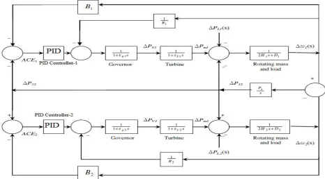
The basic block diagram of two area power system connected by tie line with ACE and PID controller is shown in fig.1.
Fig.1 : LFC for a two-area power system with ACE loops and PID controller.
III. DESIGN OF CONTROLLER
Now days the use of conventional integral controllers is very rare in Load Frequency Control of power system as they produce very slow dynamic response for the system. With the wide development of control system, many different controllers have been invented which are much more effective than integral controllers.
PID controller is one of such controllers. The desired performance can be obtained by proper tuning of the PID controller parameters.
between a measured process variable and a desired set point. The controller attempts to minimize the error by adjusting the process through use of a manipulated variable.
The PID controller involves three separate constant parameters and is accordingly sometimes called three-term control: the proportional, the integral and derivative values, denoted P, I, and D. Simply put, these values can be interpreted in terms of time: P depends on the present error, I on the accumulation of past errors, and D is a prediction of future errors, based on current rate of change.
Some applications may require using only one or two actions to provide the appropriate system control. This is achieved by setting the other parameters to zero. A PID controller will be called a PI, PD, P or I controller in the absence of the respective control actions. PI controllers are fairly common, since derivative action is sensitive to measurement noise, whereas the absence of an integral term may prevent the system from reaching its target value due to the control action.
PID controllers were subsequently developed in automatic ship steering. One of the earliest examples of a PID-type controller was developed by Elmer Sperry in 1911, while the first published theoretical analysis of a PID controller was by Russian American engineer Nicolas Minorsky.
The PID control scheme is named after its three correcting terms, whose sum constitutes the manipulated variable (MV). The proportional, integral, and derivative terms are summed to calculate the output of the PID controller. Defining U(t) as the controller output, the final form of the PID controller is given in equation (1).
U(t) = MV(t) = KP e(t) + Ki ∫0
( )
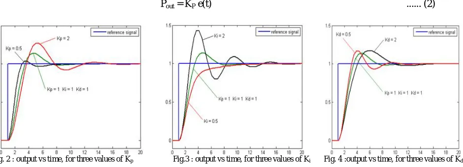
dt + Kd ( ) …..(1)Proportional Term: The proportional term produces an output value that is proportional to the current error value. The proportional response can be adjusted by multiplying the error by a constant Kp, called the proportional gain constant. The proportional term is given in equation (2).
Pout = KP e(t)
... (2)
Fig. 2 : output vs time, for three values of Kp Fig.3 : output vs time, for three values of Ki Fig. 4 :output vs time, for three values of Kd
Integral Term: The contribution from the integral term is proportional to both the magnitude of the error and the duration of the error. The integral in a PID controller is the sum of the instantaneous error over time and gives the accumulated offset that should have been corrected previously. The accumulated error is then multiplied by the integral gain Ki and added to the controller output. The integral term is given by equation (3).
Iout = Ki ∫ ( ) dt ….. (3)
Derivative term: The derivative of the process error is calculated by determining the slope of the error over the time and multiplying this rate of change by the derivative gain Kd. The magnitude of the contribution of the derivative term
to the overall control action is termed the derivative gain, Kd. The derivative term is given by equation (4).
Dout = Kd ( ) ….. (4)
Derivative action predicts system behaviour and thus improves settling time and stability of the system. An ideal derivative is not causal, so that implementations of PID controllers include an additional low pass filtering for the derivative term to limit the high frequency gain and noise. Derivative action is seldom used in practice because of its variable impact on system stability in real-world applications. Fig. 4 shows the effect of derivative gain Kd.
Tuning: Tuning a control loop is the adjustment of its control parameters (proportional gain, integral gain and derivative gain) to the optimum values for the desired control response. Stability (no unbounded oscillation) is a basic requirement, but beyond that, different systems have different behaviour, different applications have different requirements and requirements may conflict with each other.
PID tuning is a difficult problem even though there are only three parameters and its principle is simple to describe, because it must satisfy complex criteria within the limitations of PID control. There are accordingly various methods for tuning and more sophisticated techniques are the subject of patents. This section describes some methods for tuning of controller parameters in PID controllers, that is, methods for finding proper values of Kp, Ki and Kd.
Designing and tuning a PID controller appears to be conceptually intuitive, but can be hard in practice, if multiple and often conflicting objectives such as short transient and high stability are to be achieved. PID controllers often provide acceptable control using default tunings, but performance can generally be improved by careful tuning and performance may be unacceptable with poor tuning. Usually, initial designs need to be adjusted repeatedly through computer simulations until the closed-loop system performs as desired.
Some processes have a degree of nonlinearity and so parameters that work well at full-load conditions don't work when the process is starting up from no-load. This can be corrected by gain scheduling (using different parameters in different operating regions).
Stability: If the PID controller parameters the gains of the proportional, integral and derivative terms are chosen incorrectly, the controlled process input can be unstable, i.e., its output diverges, with or without oscillation and is limited only by saturation or mechanical breakage. Instability is caused by excess gain, particularly in the presence of significant lag.Generally, stabilization of response is required and the process must not oscillate for any combination of process conditions and set points, though sometimes marginal stability or bounded oscillation is acceptable or desired.
Optimum Behaviour: The optimum behaviour on a process change or set point change varies depending on the application. Two basic requirements are regulation or disturbance rejection means staying at a given set point and command tracking or implementing set point changes, these refer to how well the controlled variable tracks the desired value. Specific criteria for command tracking include rise time and settling time. Some processes must not allow an overshoot of the process variable beyond the set point and other processes must minimize the energy expended in reaching a new set point.
IV.TUNING OF PID CONTROLLER BY ZIEGLER-NICHOLS (Z-N) METHOD
The Ziegler–Nichols tuning method is a heuristic method of tuning a PID controller. It was developed by John G. Ziegler and Nathaniel B. Nichols.
Determining the ultimate gain value Ku is accomplished by finding the value of the proportional gain that causes the control loop to oscillate indefinitely at steady state. This means that the gains from the I and D controller are set to zero so that the influence of P can be determined. It tests the robustness of the Kp value so that it is optimized for the controller. Another important value associated with this proportional control tuning method is the ultimate period (Tu). The ultimate period is the time required to complete one full oscillation while the system is at steady state. These two parameters, Ku and Tu, are used to find the loop-tuning constants of the controller (P, PI, or PID). To find the values of these parameters and to calculate the tuning constants, use the following procedure:
1. Remove integral and derivative action. Set integral gain (Ki) to zero value and set the derivative controller gain (Kd) to zero.
2. Create a small disturbance in the loop by changing the set point. Adjust the proportional, increasing and/or decreasing, the gain until the oscillations have constant amplitude.
3. Record the gain value (Ku) and period of oscillation (Tu).
4. Put these values into the Ziegler-Nichols closed loop equations and determine the necessary settings for the controller.
Table 2 : PID controller parameters using Ziegler–Nichols Method
Control Type Kp Ki Kd
P 0.5 Ku - -
PI 0.45 Ku 1.2Kp/Tu -
PD 0.8 Ku - Kp Tu /8
PID 0.60 Ku 2Kp/ Tu Kp Tu /8
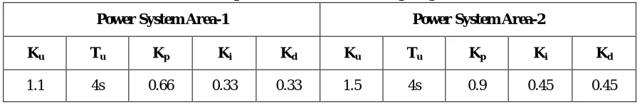
For power system area-1
Ku=1.1 and Tu= 4s, Therefore Kp= 0.6 Ku= 0.66, Ki= 2 Kp/Tu = 0.33 and Kd= KpTu/8 = 0.33
For power system area-2
Ku=1.5 and Tu= 4s, Therefore Kp= 0.6 Ku= 0.9, Ki= 2 Kp/Tu = 0.45 and Kd= KpTu/8 = 0.45
Table 3 : PID controller parameters calculated using Ziegler–Nichols Method
V. TUNING OF PID CONTROLLER BY SIMPLEX SEARCH METHOD
There are many methods available for tuning of PID controller. All these methods are used as initial guess for PID controller parameter setting. Later these settings are improved by fine tuning. Now a days simulation softwares are widely popular. MATLAB Simulink is one of them. Hence the advantage of simulation tools taken and used a method for tuning of PID controllers using simulation.
When a Simulink model is design to meet requirements for optimizing parameters, Simulink Design Optimization software automatically converts the requirements into a constrained optimization problem and then solves the problem using optimization techniques. The constrained optimization problem iteratively simulates the Simulink model,
Power System Area-1 Power System Area-2
Ku Tu Kp Ki Kd Ku Tu Kp Ki Kd
compares the results of the simulations with the constraint objectives and uses optimization methods to adjust tuned parameters to better meet the objectives.
Simplex Search Method Problem Formulations: The Simplex Search method uses the Optimization Toolbox function fminsearch and fminbnd to optimize model parameters to meet design requirements. fminbnd is used if one scalar parameter is being optimized otherwise fminsearch is used. Parameter bounds cannot used with fminsearch.
Several options for the optimization can be set. These options include the optimization methods and the tolerances the methods use. Both the Method and Algorithm options in the Optimization method area define the optimization method. The following results were obtained from Simplex tuning method as shown in table 4.
Table 4: PID controller parameters calculated using Simplex method
Power System Area-1 Power System Area-2
Kp Ki Kd Kp Ki Kd
0.4221 1.2113 0.3295 0.9 0.45 0.45
VI. RESULT AND DISCUSSION
In this section simulated two area power system connected by the tie line with (i) Only AGC loop (ii) AGC with ACE loop (integral control only) (iii) LFC with PID controller are shown. Also the PID controller whose parameters are tuned with different methods is applied and results are shown.
Fig 5. : f1 and f2 with AGC loop Fig.6 : f1 and f2 with AGC-ACE loop
Fig. 5 shows the frequency deviation in area-1 and area-2 with only AGC loop. It is seen that there is always deviation in frequencies of both areas after the load change. f1 and f2 never set to zero. Fig. 6 shows the frequency deviation in
area-1 and area-2 with AGC-ACE loop. It can be seen that there are number of oscillations and it take a large time to set f1 and f2 to zero or very near to zero.
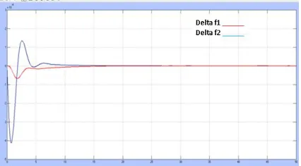
Fig. 7 and fig. 8 shows the frequency deviation in area-1 and area-2 with PID controller tuned by Z-N method and simplex method respectively. It is seen deviation in frequencies of both areas (f1 and f2) set to zero in very small time after the load change. Also there are very few oscillations. It means that both transient and steady state response improve.
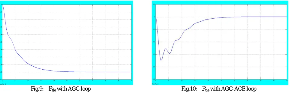
Fig.9: Ptiewith AGC loop Fig.10: Ptiewith AGC-ACE loop
Fig. 9 shows Tie line power deviation with only AGC loop. It is seen that there is always deviation in tie line power of after the load change. Ptie never set to pre set value. Fig. 10 shows the tie line power deviation with AGC-ACE loop.
It can be seen that there are number of oscillations and it take a large time to set Ptie to pre set value or very near to it.
Fig.11: Ptiewith PID controller tuned by Z-N method Fig.12: Ptiewith PID controller tuned by Simplex method
Fig. 11 and fig. 12 shows Ptie with PID controller tuned by Z-N method and simplex method respectively. It is seen
deviation in tie line power (Ptie) set to its pre defined value in very small time after the load change. Also there are
very few oscillations. It means that both transient and steady state response improve.
Table 5 : Time response specifications for f1
S.No Tuning Method
PID Controller -1 PID Controller -2
Mp Tp Tr Ts Response Kp Ki Kd Kp Ki Kd
1 Z-N 0.66 0.33 0.33 0.9 0.45 0.45 -0.8*10-4 2s 27s 27s Stable
Here table 5 shows the comparative study of time response specifications for deviation in frequency of area-1((f1) with PID controller whose parameters are tuned by Z-N method and simplex method.
Table 6 : Time response specifications for f2
The table 6 shows the comparative study of time response specifications for deviation in frequency of area-2((f2) for load change with PID controller whose parameters are tuned by Z-N method and simplex method.
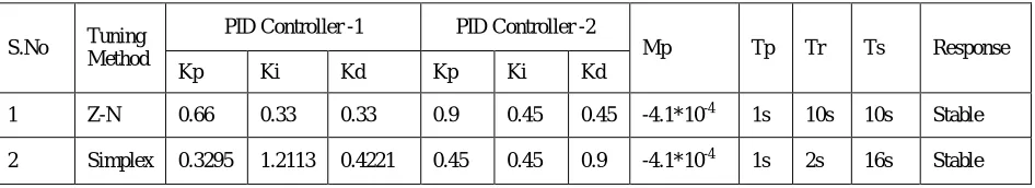
Table 7 : Time response specifications for Ttie
The table 7 shows the comparative study of time response specifications for deviation in tie line power ((Ptie) with
PID controller whose parameters are tuned by Z-N method and simplex method.
The change in load powers which are the input disturbances are taken as, PL1 = 0.01 pu, PL2 = 0.00 pu for all the
cases.
VII. CONCLUSION
Model of a two area interconnected power system has been developed with different area characteristics for modern and conventional control strategies. In LFC systems it is important to keep the power system frequency and the inter area tie line power as close as possible to the scheduled values. It has been shown that the use of simple integral controller is incapable of obtaining good dynamic performance.
The PID controllers are well known and are widely used in power system and control systems to damp system oscillations, increase stability and reduce steady state error as they are simple to realize and easily tuned. It is seen that if the proper tuning of parameter of PID controller is done, the area frequencies could brought back to its predefined value or very nearer to its predefined value with acceptable tolerance so as the tie line power in minimum time, when the is sudden change in load occurs .
REFERENCES
[1] A. Khodabakhshian and N. Golbon, “Unified PID design for load frequency control”, in Proc. 2004 IEEE Int. Conf. Control Applications (CCA), Taipei, Taiwan, Sep. 2004.
[2] A. M. Stankovic, G. Tadmor, and T. A. Sakharuk, “On robust control analysis and design for load frequency regulation”, IEEE Trans. Power Syst., vol. 13, no. 2, pp. 449–455, May 1998.
[3] A. Rubaai and V. Udo, “An adaptive control scheme for LFC of multi area power systems. Part I: Identification and functional design, Part-II: Implementation and test results by simulation”, Elect. Power Syst. Res., vol. 24, no. 3, pp. 183–197, Sep. 1992.
[4] IEEE PES Working Group, “Hydraulic turbine and turbine control models for system dynamic Studies”, IEEE Trans. Power Syst., vol. PWRS-7, no. 1, pp. 167–174, Feb. 1992.
[5] C. Concordia and L.K. Kirchmayer, “Tie line power and frequency control of electric power systems”, Amer. Inst. Elect. Eng. Trans., Pt. II, Vol. 72, pp. 562 572, Jun. 1953.
S.No Tuning Method
PID Controller -1 PID Controller -2
Mp Tp Tr Ts Response Kp Ki Kd Kp Ki Kd
1 Z-N 0.66 0.33 0.33 0.9 0.45 0.45 -4.1*10-4 1s 10s 10s Stable
2 Simplex 0.3295 1.2113 0.4221 0.45 0.45 0.9 -4.1*10-4 1s 2s 16s Stable
S.No Tuning Method
PID Controller -1 PID Controller -2
Mp Tp Tr Ts Response Kp Ki Kd Kp Ki Kd
1 Z-N 0.66 0.33 0.33 0.9 0.45 0.45 -1.1*10-3 4s 25s 25s Stable
[6] C. E. Fosha and O. I. Elgerd, “The megawatt -frequency control problem: A new approach via optimal control theory”, IEEE Trans. Power App. Syst., vol. PAS-89, no. 4, pp. 563–567, 1970.
[7] D. Das, J. Nanda, M. L. Kothari, and D. P. Kothari, “Automatic generation control of Hydro Thermal system with new area control error considering generation rate constraint”, Elect. Mach. Power Syst., vol. 18, no. 6, pp. 461– 471, Nov./Dec. 1990.
[8] E. C. Tacker, T. W. Reddoch, O. T. Pan, and T. D. Linton, “Automatic generation Control of electric energy systems—A simulation study”, IEEE Trans. Syst. Man Cybern., vol. SMC-3, no. 4, pp. 403–405, Jul. 1973.
[9] E.Tacker, C.Lee,T.Reddoch, T.Tan, P.Julich, “Optimal Control of Interconnected Electric Energy System- A new formulation” ,Proc. IEEE, 1972.
[10] IEEE PES Committee Report, “Current operating problems associated with automatic generation control”, IEEE Trans. Power App. Syst., vol. PAS-98, Jan./Feb. 1979.
[11] N. Cohn, “Some aspects of tie-line bias control on interconnected power systems”, Amer. Inst. Elect. Eng. Trans., Vol. 75, pp. 1415-1436, Feb. 1957.
[12] N. Jaleeli, L. S. Vanslyck, D. N. Ewart, L. H. Fink, and A. G. Hoffmann, “Understanding automatic generation control”, IEEE Trans. Power App.Syst. vol. PAS-7, no. 3, pp. 1106–1122, Aug. 1992.
[13] O. I. Elgerd and C. Fosha, “Optimum megawatt frequency control of multi area electric energy systems”, IEEE Trans. Power App. Syst., vol. PAS-89, no. 4, pp. 556–563, Apr. 1970.
[14] R. K. Cavin, M. C. Budge Jr., P. Rosmunsen, “An Optimal Linear System Approach to Load Frequency Control”, IEEE Trans. On Power Apparatus and System, PAS-90, pp. 2472-2482, Nov./Dec. 1971.
[15] R. K. Green, “Transformed automatic generation control”, IEEE Trans. Power Syst., vol. 11, no. 4, pp. 1799–1804, Nov. 1996.
[16] Yogendra Arya, Narendra Kumar, S.K. Gupta, “Load Frequency Control of a Four- Area Power System using Linear Quadratic Regulator”, IJES Vol.2, PP.69-76, 2012.
[17] Yogesh B. hote et. al., “Load Frequency Control in Power Systems via Internal Model Control Scheme and Model-Order Reduction”, IEEE Transactions On Power Systems, Vol. 28, No. 3, pp. 2749-2757, August 2013.
[18] Wen Ten, “Unified Tuning of PID Load Frequency Controller for Power Systems via IMC”, IEEE Transactions On Power Systems, Vol. 25, No. 1, pp. 341-350, February 2010.
[19] Y. H. Moon, H. S. Ryu, J. G. Lee, and S. Kim, “Power system load frequency control using noise-tolerable PID feedback”, in Proc. IEEE Int. Symp. Industrial Electronics (ISIE), vol. 3, pp. 1714–1718, Jun. 2001.
[20] V. Ganesh et. al., “LQR Based Load Frequency Controller for Two Area Power System”, International Journal of Advanced Research in Electrical, Electronics and Instrumentation Engineering Vol. 1, Issue 4, pp. 262-269, October 2012.