Volume 2006, Article ID 32592, Pages1–12 DOI 10.1155/ASP/2006/32592
End-to-End Rate-Distortion Optimized MD Mode Selection for
Multiple Description Video Coding
Brian A. Heng,1John G. Apostolopoulos,2and Jae S. Lim1
1Massachusetts Institute of Technology, Cambridge, MA 02139, USA
2Streaming Media Systems Group, Hewlett-Packard Labs, Palo Alto, CA 94304, USA
Received 10 March 2005; Revised 13 August 2005; Accepted 1 September 2005
Multiple description (MD) video coding can be used to reduce the detrimental effects caused by transmission over lossy packet networks. A number of approaches have been proposed for MD coding, where each provides a different tradeoffbetween compres-sion efficiency and error resilience. How effectively each method achieves this tradeoffdepends on the network conditions as well as on the characteristics of the video itself. This paper proposes an adaptive MD coding approach which adapts to these conditions through the use of adaptive MD mode selection. The encoder in this system is able to accurately estimate the expected end-to-end distortion, accounting for both compression and packet loss-induced distortions, as well as for the bursty nature of channel losses and the effective use of multiple transmission paths. With this model of the expected end-to-end distortion, the encoder selects between MD coding modes in a rate-distortion (R-D) optimized manner to most effectively tradeoffcompression efficiency for error resilience. We show how this approach adapts to both the local characteristics of the video and network conditions and demonstrates the resulting gains in performance using an H.264-based adaptive MD video coder.
Copyright © 2006 Brian A. Heng et al. This is an open access article distributed under the Creative Commons Attribution License, which permits unrestricted use, distribution, and reproduction in any medium, provided the original work is properly cited.
1. INTRODUCTION
Streaming video applications often require error-resilient video coding methods that are able to adapt to current net-work conditions and to tolerate transmission losses. These applications must be able to withstand the potentially harsh conditions present on best-effort networks like the Internet, including variations in available bandwidth, packet losses, and delay.
Multiple description (MD) video coding is one approach that can be used to reduce the detrimental effects caused by packet loss on best-effort networks [1–7]. In a multiple de-scription system, a video sequence is coded into two or more complementary streams in such a way that each stream is in-dependently decodable. The quality of the received video im-proves with each received description, but the loss of any one of these descriptions does not cause complete failure. If one of the streams is lost or delivered late, the video playback can continue with only a slight reduction in overall quality. For an in-depth review of MD coding for video communications see [8].
There have been a number of proposals for MD video coding each providing their own tradeoff between com-pression efficiency and error resilience. Previous MD cod-ing approaches applied a scod-ingle MD technique to an entire
sequence. However, the optimal MD coding method will de-pend on many factors including the amount of motion in the scene, the amount of spatial detail, desired bitrates, error recovery capabilities of each technique, current network con-ditions, and so forth. This paper examines the adaptive use of multiple MD coding modes within a single sequence. Specifi-cally, this paper proposes an adaptive MD coder which selects among MD coding modes in an end-to-end rate-distortion (R-D) optimized manner as a function of local video charac-teristics and network conditions. The addition of the end-to-end R-D optimization is an extension of the adaptive system proposed in [9]. Some preliminary results with this approach were presented in [10].
This paper continues inSection 2with a discussion of the MD coding modes used and the advantages and disadvan-tages of each. Sections3and4present an overview of how end-to-end optimized mode selection can be achieved in MD systems. The details of the proposed system are provided in
Section 5, and experimental results are given inSection 6.
2. MD CODING MODES
· · · · · ·
Stream 1:
Stream 2:
0 2 4
1 3 5
(a) Single description coding (SD)
· · · · · ·
Stream 1:
Stream 2:
0 2 4
1 3 5
(b) Temporal splitting (TS)
a b
Even lines Odd lines
· · · · · ·
Stream 1:
Stream 2:
0a 1a 2a 3a 4a
0b 1b 2b 3b 4b
(c) Spatial splitting (SS)
· · · · · ·
Stream 1:
Stream 2:
0 1 2 3 4
0 1 2 3 4
(d) Repetition coding (RC)
Figure1: Examined MD coding methods: (a) single description coding: each frame is predicted from the previous frame in a standard manner to maximize compression efficiency; (b) temporal splitting: even frames are predicted from even frames and odd from odd; (c) spatial splitting: even lines are predicted from even lines and odd from odd; (d) repetition coding: all coded data repeated in both streams.
these streams does not cause complete failure, and the qual-ity of the received video improves with each received descrip-tion. Therefore, even when one description is lost for a sig-nificant length of time the video playback can continue, at a slight reduction in quality, without waiting for rebuffering or retransmission.
Perhaps the simplest example of an MD video coding sys-tem is one where the original video sequence is partitioned in time into even and odd frames, which are then independently coded into two separate streams for transmission over the network. This approach generates two descriptions, where each has half the temporal resolution of the original video. In the event that both descriptions are received, the frames from each can be interleaved to reconstruct the full sequence. In the event one stream is lost, the other stream can still be straightforwardly decoded and displayed, resulting in video at half the original frame rate.
Of course, this gain in robustness comes at a cost. Tem-porally subsampling the sequence lowers the temporal cor-relation, thus reducing coding efficiency and increasing the number of bits necessary to maintain the same level of qual-ity. Without losses, the total bitrate necessary for this MD system to achieve a given distortion is generally higher than the corresponding rate for a single stream encoder to achieve the same distortion. This is a tradeoffbetween coding effi -ciency and robustness. However, in an application where we stream video over a lossy packet network, it is not so much a question of whether it is useful to give up some amount of efficiency for an increase in reliability as it is a question of finding the most effective way to achieve this tradeoff.
This paper proposes adaptive MD mode selection in which the encoder switches between different coding modes
within a sequence in an intelligent manner. To illustrate this idea, the system discussed in this paper uses a combination of four simple MD modes: single description coding (SD), temporal splitting (TS), spatial splitting (SS), and repetition coding (RC), seeFigure 1. This section continues by describ-ing these methods and their advantages and disadvantages; seeTable 1.
Single description (SD) coding represents the typical coding approach where each frame is predicted from the pvious frame in an attempt to remove as much temporal re-dundancy as possible. Of all the methods presented here, SD coding has the highest coding efficiency and the lowest re-silience to packet losses. On the other extreme, repetition coding (RC) is similar to the SD approach except the data is transmitted once in each description. This obviously leads to poor coding efficiency, but greatly improves the overall er-ror resilience. As long as both descriptions of a frame are not lost simultaneously, there will be no effect on decoded video quality. The remaining two modes provide additional trade-offs between error resilience and coding efficiency. The tem-poral splitting (TS) mode effectively partitions the sequence along the time dimension into even and odd frames. Even frames are predicted from even and odd frames from odd frames. Similarly, in spatial splitting (SS), the sequence is par-titioned along the spatial direction into even and odd lines. Even lines are predicted from even lines and odd from odd.
Table1: List of MD coding modes along with their relative advantages and disadvantages.
MD mode Description Advantages Disadvantages
SD Single description coding Highest coding efficiency of all methods Least resilience to errors
TS Temporal splitting
Good coding efficiency with better error Increased temporal distance reduces the resilience than SD coding. Works well in effectiveness of temporal prediction leading to regions with little or no motion a decrease in coding efficiency
SS Spatial splitting
High resilience to errors with better coding Field coding leads to decreased coding
efficiency than RC. Works well in regions with efficiency, with typically lower coding efficiency some amount of motion than TS mode
RC Repetition coding
Highest resilience to errors of all the methods. Repetition of data is costly leading to low The loss of either stream has no effect coding efficiency
on decoded quality
and error resilience. This set of modes examines a wide range on the compression efficiency/error resilience spec-trum, from most efficient single description coding to most resilient repetition coding. Finally, these approaches are all fairly simple both conceptually and from a complexity stand-point. Conceptually, it is possible to quickly understand where each one of these modes might be most or least ef-fective, and in terms of complexity, the decoder in this sys-tem is not much more complicated than the standard video decoder. It is important to note that additional MD modes of interest may be straightforwardly incorporated into the adaptive MD encoding framework and the associated models for determining the optimized MD mode selection. In addi-tion, it is also possible to account for improved MD decoder processing which may lead to reduce distortion from losses (e.g., improved methods of error recovery where a damaged description is repaired by using an undamaged description [1,11]), and thereby effect the end-to-end distortion estima-tion performed as part of the adaptive MD encoding.
3. OPTIMIZED MD MODE SELECTION
Each approach to MD coding trades off some amount of
compression efficiency for an increase in error resilience. How efficiently each method achieves this tradeoffdepends on the quality of video desired, the current network condi-tions, and the characteristics of the video itself. Most prior research in MD coding involved the design and analysis of novel MD coding techniques, where a single MD method is applied to the entire sequence; this approach is taken so as to evaluate the performance of each MD method. However, it would be more efficient to adaptively select the best MD method based on the situation at hand. Since the encoder in this system has access to the original source, it is possible to calculate the rate-distortion statistics for each coding mode and select between them in an R-D optimized manner.
The main question then is how to make the decision be-tween different modes. Lagrangian optimization techniques can be used to minimize distortion subject to a bitrate con-straint [12]. However, this approach assumes the encoder has full knowledge of the end-to-end distortion experienced by the decoder. When transmitted over a lossy channel, the
end-to-end distortion consists of two terms; (1) known dis-tortion from quantization and (2) unknown disdis-tortion from random packet loss. The unknown distortion from losses can only be determined in expectation due to the random nature of losses. Modifying the Lagrangian cost function to account for the total end-to-end distortion gives the following:
J(λ)=Diquant+E Diloss
+λRi. (1)
Here,Riis the total number of bits necessary to code region
i,Dquanti is the distortion due to quantization, andDlossi is
a random variable representing the distortion due to packet losses. Thus, the expected distortion experienced by the de-coder can be minimized by coding each region with all avail-able modes and choosing the mode which minimizes this La-grangian cost.
Calculating the expected end-to-end distortion is not a straightforward task. The quantization distortionDquanti and
bitrate Ri are known at the encoder. However, the channel distortionDilossis difficult to calculate due to spatial and
tem-poral error propagation. In [13], the authors show how to es-timate expected distortion in a pixel-accurate recursive man-ner for SD and Bernoulli losses. In the next section, we dis-cuss this approach and the extensions necessary to apply it to the current problem of MD coding over multiple paths with Gilbert (bursty) losses.
4. MODELING EXPECTED DISTORTION IN MULTIPLE DESCRIPTION STREAMS
for optimal intra/inter mode selection. Here, the expected distortion for any pixel location is calculated recursively as follows. Suppose fi
nrepresents the original pixel value at
lo-cationiin framen, and fi
nrepresents the reconstruction of
the same pixel at the decoder. The expected distortiondi nat
that location can then be written as
di n=E
fi
n−fni 2
= fi2
n −2fniE
fi n
+Efi2
n
. (2)
At the encoder, the value fi
nis known and the value fni is a
random variable. So, the expected distortion at each location can be determined by calculating the first and second mo-ment of the random variable fi
n.
If we assume the encoder uses full pixel motion estima-tion, each correctly received pixel value can be written asfi
n= ei
n+ f j
n−1, where f
j
n−1 represents the pixel value in the pre-vious frame which has been used for motion,-compensated prediction andei
nrepresents the quantized residual (in the
case of intra pixels, the prediction is zero and the residual is just the quantized pixel value). The first moment of each re-ceived pixel can then be recursively calculated by the encoder as follows
Efni|received
=eni+E
fn−j 1
. (3)
If we assume the decoder uses frame copy error concealment, each lost pixel is reconstructed by copying the pixel at the same location in the previous frame. Thus, the first moment of each lost pixel is
Efi n|lost
=Efi
n−1
. (4)
The total expectation can then be calculated as
Efi n
=P(received)Efi
n|received
+P(lost)Efi n|lost
.
(5) The calculations necessary for computing the second mo-ment of fi
ncan be derived in a similar recursive fashion.
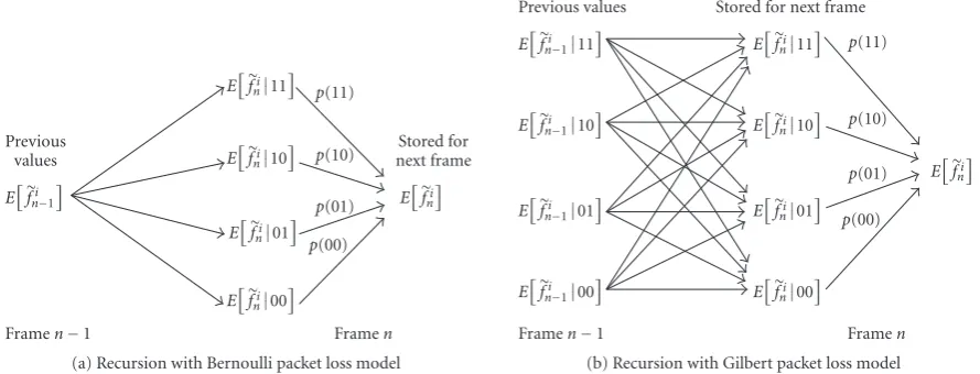
In [16], this ROPE model is extended to a two-stream multiple description system by recognizing the four possible loss scenarios for each frame: both descriptions are received, one or the other, description is lost, or both descriptions are lost. For notational convenience, we will refer to these out-comes as 11, 10, 01, and 00 respectively. The conditional ex-pectations of each of these four possible outcomes are recur-sively calculated and multiplied by the probability of each oc-curring to calculate the total expectation,
Efi n
=P(11)Efi n|11
+P(10)Efi n|10
+P(01)Efi n|01
+P(00)Efi n|00
.
(6)
Graphically, this can be depicted as shown inFigure 3(a). The first moments of the random variablesfi
n−1as calculated in the previous frame are used to calculate the four interme-diate expected outcomes which are then combined together using (6) and stored for future frames. Again, the second mo-ment calculations can be computed in a similar manner.
These previous methods have assumed a Bernoulli-independent packet loss model where the probability that any packet is lost is independent of any other packet. How-ever, the idea can be modified for a channel with bursty packet losses as well. Recent work has identified the im-portance of burst length in characterizing error resilience schemes, and that examining performance as a function of burst length is an important feature for comparing the relative merits of different error-resilient coding methods [11,17,18].
For this system, we have extended the MD ROPE ap-proach to account for bursty packet loss. Here we use a two-state Gilbert loss model, but the same approach could be used for any multistate loss model including those with fixed burst lengths. We use the Gilbert model to simulate the na-ture of bursty losses where packet losses are more likely if the previous packet has been lost. This can be represented by the Markov model shown inFigure 2assumingp0< p1.
The expected value of any outcome in a multistate packet loss model can be calculated by computing the expectation conditioned on transitioning from one outcome to another multiplied by the probability of making that transition. For the two-state Gilbert model, this idea can be roughly de-picted as shown inFigure 3(b). For example, assumeTAB
rep-resents the event of transitioning from outcomeA at time
n−1 to outcomeBat timen, andP(TB
A) represents the
prob-ability of making this transition. Then the expected value of outcome 11 can be computed as shown in (7),
Efi n|11
=PT11 11
·Efi
n|T1111
+PT11 10
·Efi
n|T1011
+PT11 01
·Efi
n|T0111
+PT11 00
·Efi
n|T0011
.
(7)
The remaining three outcomes can be computed in a similar manner. Due to the Gilbert model, the probability of tran-sitioning from any outcome at timen−1 to any other out-come at timenchanges depending on which outcome is cur-rently being considered. For instance, when computing the expected value of outcome 00, the result when both streams are lost, the probability that the previous outcome was 10, 01, or 00 is much higher than when computing the expected value of outcome 11. Since the transitional probabilities vary from outcome to outcome, it is not possible to combine the four expected outcomes into one value as can be done in the Bernoulli case. The four values must be stored separately for future use as shown inFigure 3(b). Once again, the second moment values can be computed using a similar approach.
p0
1−p1
0 1
1−p0 p1
State 0: packet received State 1: packet lost
Average packet loss rate
=1 + p0 P0−p1
Expected burst length
= 1
1−p1
Figure2: Gilbert packet loss model. Assumingp0< p1, the probability of each packet being lost increases if the previous packet was lost.
This causes bursty losses in the resulting stream.
Efni−1
Efi n
Efi n11
Efi n10
Efi n01
Efi n00
p(11)
p(10)
p(01)
p(00)
Stored for next frame Previous
values
Framen−1 Framen
(a) Recursion with Bernoulli packet loss model
Efi n
Efi n−111
Efi n−110
Efni−101
Efni−100
Framen−1
Efi n11
Efi n10
Efi n01
Efi n00
p(11)
p(10)
p(01)
p(00)
Framen
Stored for next frame Previous values
(b) Recursion with Gilbert packet loss model
Figure3: Conceptual computation of first moment values in MD ROPE approach: (a) Bernoulli case: the moment values from the previous frame are used to compute the expected values in each of the four possible outcomes which are then combined to find the moment values for the current frame; (b) Gilbert losses: due to the Gilbert model, the probability of transitioning from any one outcome at timen−1 to any other outcome at timenchanges depending on which outcome is currently being considered. Thus, the four expected outcomes cannot be combined into one single value as was done in the Bernoulli case. Each of these four values must be stored separately for future calculations.
vector accuracy and more sophisticated error concealment methods by using the techniques proposed in [19] for esti-mation of cross-correlation terms. Specifically, each correla-tion termE[XY] is estimated by
E[XY]=E[X]
E[Y]E
Y2. (8)
Figure 4demonstrates the performance of the above ap-proach in tracking the actual distortion experienced at the decoder. Here we have coded the Foreman and Carphone test sequences at approximately 0.4 bits per pixel (bpp) with the H.264 video codec using the SD approach mentioned in
Section 2. The channel has been modeled by a two path chan-nel, where the paths are symmetric with Gilbert losses at an average packet loss rate of 5% and expected burst length of 3 packets. The expected distortion as calculated at the encoder using the above model has been plotted relative to the actual distortion experienced by the decoder. This actual distortion was calculated by using 1 200 different packet loss traces and averaging the resulting squared-error distortion. As shown in both of these sequences, the proposed model is able to track
the end-to-end expected distortion quite closely. Also shown in this figure for reference is the quantization only distortion (with no packet losses).
5. MD SYSTEM DESIGN AND IMPLEMENTATION
The system described in this paper has been implemented based on the H.264 video coding standard using quarter-pixel motion vector accuracy and all available intra- and in-terprediction modes [20]. We have used reference software version 8.6 for these experiments with modifications to sup-port adaptive mode selection. Due to the in-loop deblocking filter used in H.264, the current macroblock will depend on neighboring macroblocks within the frame, including blocks which have yet to be coded. This deblocking filter has been turned offin our experiments to remove this causality issue and simplify the problem.
The adaptive mode selection is performed on a mac-roblock basis using the Lagrangian techniques discussed in
Quant only Actual Expected
0 50 100 150 200 250 300 350 Frame
26 28 30 32 34 36 38
PSNR
(dB)
(a) Foreman sequence
Quant only Actual Expected
0 50 100 150 200 250 300 350
Frame 27
29 31 33 35 37 39 41
PSNR
(dB)
(b) Carphone sequence
Figure4: Comparison between actual and expected end-to-end PSNR: (a) Foreman sequence; (b) Carphone sequence. This figure demon-strates the ability of this model to track the actual end-to-end distortion, where the expected and actual distortion curves are roughly on top of each other. Also shown in this figure is the quantization only distortion which shows the distortion from compression and without any packet loss.
both traditional coding decisions (e.g., inter versus intra cod-ing) as well as for selecting one of the possible MD modes.
As mentioned in Section 2, the current system uses a combination of four possible MD modes: single description coding (SD), temporal splitting (TS), spatial splitting (SS), and repetition coding (RC). Note that when coded in a non-adaptive fashion, each method (SD, TS, SS, RC) is still per-formed in an R-D optimized manner as mentioned above. All of the remaining coding decisions, including inter ver-sus intra coding, are made to minimize the end-to-end dis-tortion. For instance, the RC mode is not simply a straight-forward replica of the SD mode. The system recognizes the improved reliability of the RC mode and elects to use far less intra-coding allowing more intelligent allocation of the avail-able bits. Also, it was necessary to modify the H.264 codec to support macroblock level adaptive interlaced coding in or-der to accommodate the spatial splitting mode. The tempo-ral splitting mode, however, was implemented using the stan-dard compliant reference picture selection available in H.264. The packetization of data differs slightly for each mode (seeFigure 5). In both the SD or TS approaches, all data for a frame is placed into a single packet. The even frames are then sent along one stream and the odd frames along the other. While in the SS and RC approaches, data from a single frame is coded into packets placed into both streams. For SS, even lines are sent in one stream and odd lines in the other, while for RC all data is repeated in both streams. Therefore, for SD and TS each frame is coded into one large packet which is sent in alternating streams, while for SS and RC each frame is coded into two smaller packets and one small packet is sent in each stream. Since the adaptive approach (ADAPT) is a combination of each of these four methods, there is typically one slightly larger packet and one smaller packet and these alternate streams between frames.
Stream 1: Stream 0:
Frame 2a Frame 1a
(a) SD and TS Stream 0:
Stream 1:
Frame 2b Frame 2a Frame 1a
Frame 1b (b) SS and RC Stream 0:
Stream 1:
2b Frame 2a Frame 1a
1b
(c) ADAPT
Figure5: Packetization of data in MD modes: (a) SD and TS: data sent along one path alternating between frames; (b) SS and RC: data spread across both streams; (c) ADAPT: combination of the two re-sulting in one slightly larger packet and one slightly smaller.
200 250 300 350 400 Frame
22 24 26 28 30 32 34 36
PSNR
(dB)
TS SD ADAPT
STD RC SS
(a) Foreman sequence
100 150 200 250 300
Frame 26
28 30 32 34 36 38 40
PSNR
(dB)
TS SD ADAPT
STD RC SS
(b) Carphone sequence
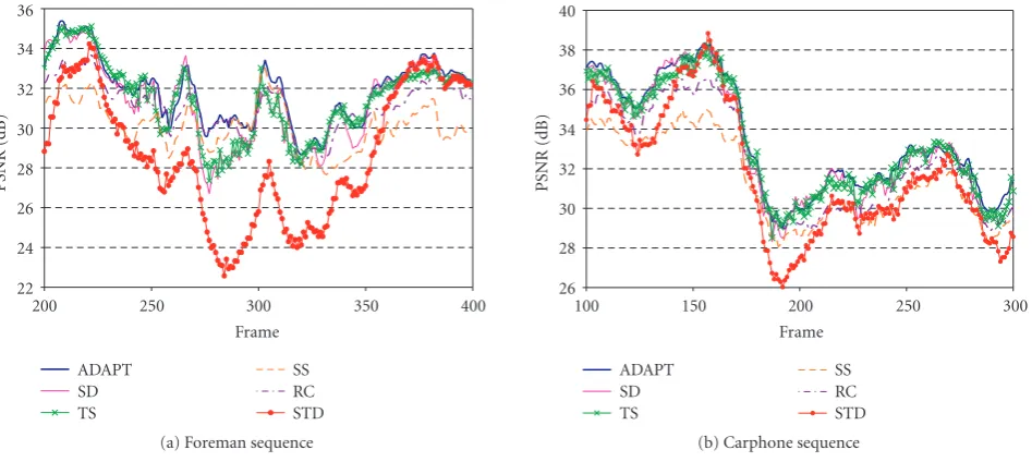
Figure6: Average distortion in each frame for ADAPT versus each nonadaptive approach. Coded at 0.4 bpp with balanced paths and 5% average packet loss rate and expected burst length of 3: (a) Foreman sequence; (b) Carphone sequence.
6. EXPERIMENTAL RESULTS
The following results have been obtained using our modified H.264 JM 8.6 codec (described above) with the Foreman and Carphone video test sequences. Both sequences are 30 frames per second at QCIF resolution. The Foreman sequence has 400 frames and the Carphone sequence has 382 frames.
To measure the actual distortion experienced at the de-coder, we have simulated a Gilbert packet loss model with packet loss rates and expected burst lengths as specified in each section below. For each of the experiments, we have run the simulation with 300 different packet loss traces and aver-aged the resulting squared-error distortion. The same packet loss traces were used throughout a single experiment to allow for meaningful comparisons across the different MD coding methods.
Each path in the system is assumed to carry 30 packets per second where the packet losses on each path are mod-eled as a Gilbert process. For wired networks, the probabil-ity of packet loss is generally independent of packet size so the variation in sizes should not generally affect the results or the fairness of this comparison. When the two paths are balanced or symmetric, the optimization automatically sends half the total bitrate across each path. For unbalanced paths, the adaptive system results in a slight redistribution of band-width as is discussed later.
In each of these experiments, the encoder is run in one of two different modes: constant bitrate encoding (CBR) or variable bitrate encoding (VBR). In the CBR mode, the quantizer and associated lambda value is adjusted on a mac-roblock basis in an attempt to keep the number of bits used in each frame approximately constant. Keeping the bitrate constant allows a number of useful comparisons between methods on a frame-by-frame basis such as those presented in Figure 6. Unfortunately, the changes in quantizer level
must be communicated along both streams in the adaptive approach which leads to some significant overhead. While this signaling information is included in the bitstream, the amount of signaling overhead is not currently incorporated in the R-D optimization decision process, hence leading to potentially suboptimal decisions with the adaptive approach. We mention this since if all of the overhead was accounted for in the R-D optimized rate control then the performance of the adaptive method would be even slightly better than shown in the current results. In the VBR mode, the quan-tizer level is held fixed to provide constant quality. In this case, there is no quantizer overhead and this approach yields results closer to the optimal performance. Since the rates of each mode may vary when in VBR mode (where the quan-tizer is held fixed), it is not possible to make a fair compari-son between different modes at a given bitrate. Therefore, in experiments where we try to make fair comparisons among different approaches at the same bitrate per frame, we op-erate in CBR mode, for example,Figure 6, and we use VBR mode to compute rate-distortion curves, like those shown in
Figure 9.
6.1. MD coding adapted to local video characteristics
We first evaluate the system’s ability to adapt to the charac-teristics of the video source. The channel in this experiment was simulated with two balanced paths each having 5% av-erage packet loss rate and expected burst length of 3 packets. The video was coded in CBR mode at approximately 0.4 bits per pixel (bpp).Figure 6demonstrates the resulting distor-tion in each frame averaged over the 300 packet loss traces for the adaptive MD method and each of its nonadaptive MD counterparts.
frame 350 to 399. Notice how the SS/RC methods work better during periods of significant motion while the SD/TS meth-ods work better as the video becomes stationary. The adap-tive method intelligently switches between the two, main-taining at least the best performance of any nonadaptive ap-proach. Since the adaptive approach adapts on a macroblock level, it is often able to do even better than the best nonadap-tive case by selecting different MD modes within a frame as well. Similar results can be seen with the Carphone se-quence. The best performing nonadaptive approach varies from frame to frame depending on the characteristics of the video. The adaptive approach generally provides the best per-formance of each of these.
Also shown inFigure 6are the results from a typical video coding approach which we will refer to as standard video coding (STD). Here, R-D optimization is only performed with respect to quantization distortion, not the end-to-end R-D optimization used in the other approaches. Instead of making inter/intra coding decisions in an end-to-end R-D optimized manner as performed by SD, it periodically in-tra updates one line of macroblocks in every other frame to combat error propagation (this update rate was chosen since the optimal intra refresh rate [21] is often approximately 1/ p, wherepis the packet loss rate).
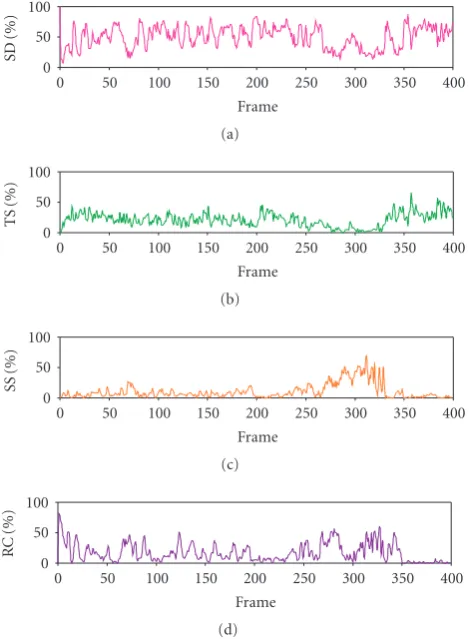
The adaptive MD approach is able to outperform opti-mized SD coding by up to 2 dB for the Foreman sequence, de-pending on the amount of motion present at the time. Note that by making intelligent decisions through end-to-end R-D optimization, the SD method examined here is able to out-perform the conventional STD method by as much as 4 or 5 dB with the Foreman sequence. The adaptive MD approach outperforms optimized SD coding by up to 1 dB with the Carphone sequence, and optimized SD coding outperforms the conventional STD approach by up to approximately 3 dB. InFigure 7, we illustrate how the mode selection varies as a function of the characteristics of the video source. Specifi-cally, we show the percentage of macroblocks using each MD mode in each frame of the Foreman sequence. From this dis-tribution of MD modes, one can roughly segment the For-man sequence into three distinct regions: almost exclusively SD/TS in the last 50 frames, mostly SS/RC from frames 250– 350, and a combination of the two during the first half. This matches up with the characteristics of the video which con-tains some amount of motion at the beginning, a fast camera scan in the middle, and is nearly stationary at the end.
6.2. MD coding adapted to network conditions
In our second experiment, we examine how the system adapts to the conditions of the network. The channel in this experiment was simulated with two balanced paths each with expected burst length of 3 packets. The video was coded in CBR mode at approximately 0.4 bits per pixel (bpp) and the average packet loss rate was varied from 0 to 10%.Figure 8
demonstrates the resulting distortion in the sequence for the adaptive MD method and each of its nonadaptive MD coun-terparts. These results were computed by first calculating the meansquared-error distortion by averaging across all the
0 50 100 150 200 250 300 350 400
Frame 0
50 100
SD
(%)
(a)
0 50 100 150 200 250 300 350 400
Frame 0
50 100
TS
(%
)
(b)
0 50 100 150 200 250 300 350 400
Frame 0
50 100
SS
(%)
(c)
0 50 100 150 200 250 300 350 400
Frame 0
50 100
RC
(%
)
(d)
Figure7: Distribution of selected MD modes used in the adap-tive method for each frame of the Foreman sequence illustrating how mode selection adapts to the video characteristics: 5% average packet loss rate, expected burst length 3.
frames in the sequence and across the 300 packet loss traces, and then computing the PSNR.
Notice how the adaptive approach achieves a perfor-mance similar to the SD approach when no losses occur, but its performance does not fall offas quickly as the aver-age packet loss rate is increased. Near the 10% loss rate, the adaptive method adjusts for the unreliable channel and has a performance closer to the RC mode. Note that the intra update rate for the STD method was adjusted in the experi-ment to be as close as possible to 1/ p, wherepis the packet loss rate, as an approximation of the optimal intra update frequency. Since this update rate could only be adjusted in an integer manner, the STD curves above tend to have some jagged fluctuations and in some cases the curves are not even monotonically decreasing. As an example, an update rate of 1/ p would imply that one should update one line of mac-roblocks every 2.22 frames at 5% loss and every 1.85 frames at 6% loss. These two cases have both been rounded to an update of one line of macroblocks every 2 frames resulting in the slightly irregular curves.
0 2 4 6 8 10 Average packet loss rate (%)
27 28 29 30 31 32 33 34 35 36 37
PSNR
(dB)
TS SD ADAPT
STD RC SS
(a) Foreman sequence
0 2 4 6 8 10
Average packet loss rate (%) 29
30 31 32 33 34 35 36 37
PSNR
(dB)
TS SD ADAPT
STD RC SS
(b) Carphone sequence
Figure8: PSNR versus average packet loss rate: (a) Foreman sequence; (b) Carphone sequence. Video coded at approximately 0.4 bpp. The average packet loss rate for this experiment was varied from 0–10%, and the expected burst length was held constant at 3 packets.
0.15 0.2 0.25 0.3 0.35 0.4 0.45 BPP
27 28 29 30 31 32 33 34
PSNR
(dB)
TS SD ADAPT
STD RC SS
(a) Foreman sequence
0.125 0.175 0.225 0.275 0.325 0.375 0.425 0.475 0.525 BPP
29 30 31 32 33 34 35
PSNR
(dB)
TS SD ADAPT
STD RC SS
(b) Carphone sequence
Figure9: End-to-end R-D performance of ADAPT and nonadaptive methods: 5% packet loss rate, expected burst length 3: (a) Foreman sequence; (b) Carphone sequence.
Table2: Comparing the distribution of MD modes in the adaptive approach at 0%, 5%, and 10% average packet loss rates. (a) Foreman sequence. (b) Carphone sequence.
MD mode 0% Loss 5% Loss 10% Loss
SD 70.87% 50.73% 43.57%
TS 18.13% 21.22% 18.97%
SS 10.81% 10.69% 10.15%
RC 0.19% 17.36% 27.31%
(a) Forman sequence.
MD mode 0% Loss 5% Loss 10% Loss
SD 67.49% 61.92% 57.51%
TS 17.29% 22.53% 20.68%
SS 15.13% 9.57% 9.19%
RC 0.09% 5.98% 12.63%
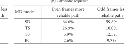
Table3: Percentage of macroblocks using each MD mode in the adaptive approach when sending over unbalanced paths.
MD mode Even frames more Odd frames less reliable path reliable path
SD 54.7% 48.3%
TS 26.5% 16.5%
SS 7.4% 12.9%
RC 11.4% 22.4%
(a) Forman sequence.
MD mode Even frames more Odd frames less reliable path reliable path
SD 64.6% 59.8%
TS 26.9% 18.0%
SS 5.9% 12.5%
RC 2.6% 9.7%
(b) Carphone sequence.
from lower redundancy methods (SD) to higher redundancy methods (RC) in an attempt to provide more protection against losses. It is interesting to point out that even at 0% loss the system does not choose 100% SD coding. The adap-tive approach recognizes that occasionally it can be more ef-ficient to predict from two frames ago than from the prior frame, so it chooses TS coding. Occasionally, it can be more efficient to code the even and odd lines of a macroblock sep-arately, so it chooses SS coding. The fact that it selects any RC at 0% loss rate is a little counterintuitive, but this results since coding a macroblock using RC changes the prediction dependencies between macroblocks. The H.264 codec con-tains many intra-frame predictions including motion vector prediction and intra-prediction. In order for the RC mode to be correctly decoded even when one stream is lost, the adaptive system must not allow RC blocks to be predicted in any manner from non-RC blocks. If RC blocks had been predicted from SD blocks, for example, the loss of one stream would affect the SD blocks which would consequently alter the RC data as well. Occasionally, prediction methods like motion vector prediction may not help and can actually re-duce the coding efficiency for certain blocks. If this is extreme enough, it can actually be more efficient to use RC, where the prediction would not be used, even though the data is then unnecessarily repeated in both descriptions.
6.3. End-to-end R-D performance
Figure 9shows the end-to-end R-D performance curves of each method. This experiment was run in VBR mode with fixed quantization levels. To generate each point on these curves, the resulting distortion was averaged across all 300 packet loss simulations, as well as across all frames of the se-quence. The same calculation was then conducted at various quantizer levels to generate each R-D curve. By switching be-tween MD methods, ADAPT is able to outperform optimized SD coding by up to 1 dB for the Foreman sequence and about 0.5 dB for the Carphone sequence. The ADAPT method is able to outperform the STD coding approach by as much as 4.5 dB with the Foreman sequence and up to 3 dB with the Carphone sequence. ADAPT is able to outperform TS, which more or less performs the second best overall, by as much as 0.5 dB.
One interesting side result here is how well RC per-forms in these experiments. Keep in mind that this is an R-D optimized RC approach, not simply the half-bitrate SD
method repeated twice. The amount of intra coding used in RC is significantly reduced relative to SD coding as the encoder recognizes the increased resilience of the RC method and chooses a more efficient allocation of bits.
6.4. Balanced versus unbalanced paths
In our final experiment, we analyze the performance of the adaptive method when used with unbalanced paths where one path is more reliable than the other. The channel con-sisted of one path with 3% average packet loss rate and an-other with 7%, both with expected burst lengths of 3 pack-ets. The video in this experiment was coded at approximately 0.4 bpp in CBR mode.Table 3shows the distribution of MD modes in even frames of the sequence versus odd frames. The even frames are those where the larger packet (seeFigure 5) is sent along the more reliable path and the smaller packet is sent along the less reliable path. The opposite is true for the odd frames. It is also interesting to compare the results fromTable 3 with those fromTable 2 at 5% balanced loss. The average of the even and odd frames fromTable 3matches closely with the values from the balanced case inTable 2.
As shown inTable 3, the system uses more SS and RC in the less reliable odd frames. These more redundant meth-ods allow the system to provide additional protection for those frames which are more likely to be lost. By doing so, the adaptive system is effectively moving data from the less reliable path into the more reliable path.Table 4shows the bitrate sent along each path in the balanced versus unbal-anced cases. In this situation, the system is shifting between 5–6% of its total rate into the more reliable stream to com-pensate for conditions on the network. Since the nonadap-tive methods are forced to send approximately half their total rate along each path, it is difficult to make a fair comparison across methods in this unbalanced situation. We are consid-ering ways to compensate for this. However, it is quite inter-esting that the end-to-end R-D optimization is able to adjust to this situation in such a manner.
7. CONCLUSIONS
Table4: Percentage of total bandwidth in each stream for balanced and unbalanced paths.
Balanced paths Unbalanced paths
Stream 1 50.5% 55.4%
Stream 2 49.5% 44.6%
(a) Forman sequence.
Balanced paths Unbalanced paths
Stream 1 50.1% 55.9%
Stream 2 49.9% 44.1%
(b) Carphone sequence.
presented here is able to accurately predict the distortion ex-perienced at the decoder taking into account both bursty packet losses and the use of multiple paths. This allows the encoder in this system to make optimized mode selections using Lagrangian optimization techniques to minimize the expected end-to-end distortion. We have shown how one such system based on H.264 is able to adapt to local char-acteristics of the video and to network conditions on multi-ple paths and have shown the potential for this adaptive ap-proach, which selects among a small number of simple com-plementary MD modes, to significantly improve video qual-ity. The results presented above demonstrate how this system accounts for the characteristics of the video source, for ex-ample, using more redundant modes in regions particularly susceptible to losses, and how it adapts to conditions on the network, for example, switching from more efficient meth-ods to more resilient methmeth-ods as the loss rate increases. The results with this approach appear quite promising, and we believe that adaptive MD mode selection can be a useful tool for reliably delivering video over lossy packet networks.
REFERENCES
[1] J. G. Apostolopoulos, “Error-resilient video compression through the use of multiple states,” inProceedings of IEEE In-ternational Conference on Image Processing (ICIP ’00), vol. 3, pp. 352–355, Vancouver, BC, Canada, September 2000. [2] C.-S. Kim and S.-U. Lee, “Multiple description coding of
mo-tion fields for robust video transmission,”IEEE Transactions on Circuits and Systems for Video Technology, vol. 11, no. 9, pp. 999–1010, 2001.
[3] A. R. Reibman, H. Jafarkhani, Y. Wang, and M. T. Orchard, “Multiple description video using rate-distortion splitting,” in Proceedings of IEEE International Conference on Image Process-ing (ICIP ’01), vol. 1, pp. 978–981, Thessaloniki, Greece, Oc-tober 2001.
[4] A. R. Reibman, H. Jafarkhani, Y. Wang, M. T. Orchard, and R. Puri, “Multiple-description video coding using motion-compensated temporal prediction,”IEEE Transactions on Cir-cuits and Systems for Video Technology, vol. 12, no. 3, pp. 193– 204, 2002.
[5] V. A. Vaishampayan and S. John, “Balanced interframe mul-tiple description video compression,” inProceedings of IEEE International Conference on Image Processing (ICIP ’99), vol. 3, pp. 812–816, Kobe, Japan, October 1999.
[6] Y. Wang and S. Lin, “Error-resilient video coding using mul-tiple description motion compensation,”IEEE Transactions on Circuits and Systems for Video Technology, vol. 12, no. 6, pp. 438–452, 2002.
[7] S. Wenger, G. D. Knorr, J. Ott, and F. Kossentini, “Error re-silience support in H.263+,”IEEE Transactions on Circuits and Systems for Video Technology, vol. 8, no. 7, pp. 867–877, 1998.
[8] Y. Wang, A. R. Reibman, and S. Lin, “Multiple description cod-ing for video delivery,”Proceedings of the IEEE, vol. 93, no. 1, pp. 57–70, 2005.
[9] B. A. Heng and J. S. Lim, “Multiple-description video coding through adaptive segmentation,” inApplications of Digital Im-age Processing XXVII, vol. 5558 ofProceedings of SPIE, pp. 105– 115, Denver, Colo, USA, August 2004.
[10] B. A. Heng, J. G. Apostolopoulos, and J. S. Lim, “End-to-end rate-distortion optimized mode selection for multiple description video coding,” in Proceedings of IEEE Interna-tional Conference on Acoustics, Speech, and Signal Processing (ICASSP ’05), Philadelphia, Pa, USA, March 2005.
[11] J. G. Apostolopoulos, “Reliable video communication over lossy packet networks using multiple state encoding and path diversity,” in Visual Communications and Image Processing (VCIP ’01), vol. 4310 ofProceedings of SPIE, pp. 392–409, San Jose, Calif, USA, January 2001.
[12] G. J. Sullivan and T. Wiegand, “Rate-distortion optimiza-tion for video compression,”IEEE Signal Processing Magazine, vol. 15, no. 6, pp. 74–90, 1998.
[13] R. Zhang, S. L. Regunathan, and K. Rose, “Video coding with optimal inter/intra-mode switching for packet loss resilience,” IEEE Journal on Selected Areas in Communications, vol. 18, no. 6, pp. 966–976, 2000.
[14] G. C ˆot´e and F. Kossentini, “Optimal intra coding of blocks for robust video communication over the Internet,”Signal Pro-cessing: Image Communication, vol. 15, no. 1-2, pp. 25–34, 1999.
[15] R. O. Hinds, T. N. Pappas, and J. S. Lim, “Joint block-based video source/channel coding for packet-switched networks,” inVisual Communications and Image Processing (VCIP ’98), vol. 3309 ofProceedings of SPIE, pp. 124–133, San Jose, Calif, USA, January 1998.
[16] A. R. Reibman, “Optimizing multiple description video coders in a packet loss environment,” inProceedings of 12th Interna-tional Packet Video Workshop (PV ’02), Pittsburgh, Pa, USA, April 2002.
[17] J. G. Apostolopoulos, W.-T. Tan, S. Wee, and G. W. Wornell, “Modeling path diversity for multiple description video com-munication,” inProceedings of IEEE International Conference on Acoustics, Speech, and Signal Processing (ICASSP ’02), vol. 3, pp. 2161–2164, Orlando, Fla, USA, May 2002.
[18] Y. J. Liang, J. G. Apostolopoulos, and B. Girod, “Analysis of packet loss for compressed video: does burst-length matter?” inProceedings of IEEE International Conference on Acoustics, Speech, and Signal Processing (ICASSP ’03), vol. 5, pp. 684–687, Hong Kong, April 2003.
[19] H. Yang and K. Rose, “Recursive end-to-end distortion estima-tion with model-based cross-correlaestima-tion approximaestima-tion,” in Proceeding of IEEE International Conference on Image Process-ing (ICIP ’03), vol. 3, pp. 469–472, Barcelona, Spain, Septem-ber 2003.
[21] K. Stuhlm¨uller, N. F¨arber, M. Link, and B. Girod, “Analysis of video transmission over lossy channels,”IEEE Journal on Se-lected Areas in Communications, vol. 18, no. 6, pp. 1012–1032, 2000.
Brian A. Hengreceived the B.S. degree in electrical engineering from University of Minnesota in 1999, and the M.S. degree in electrical engineering and computer sci-ence from Massachusetts Institute of Tech-nology in 2001. In 2005, he completed his Ph.D. in electrical engineering and com-puter science from Massachusetts Institute of Technology on multiple description cod-ing for error-resilient video
communica-tions. Brian is currently a StaffScientist in the Broadband Systems Engineering Group at Broadcom Corporation in Irvine, Calif. His current research interests include video processing/compression, video streaming, digital signal processing, and multimedia net-working.
John G. Apostolopoulosreceived his B.S., M.S., and Ph.D. degrees from Massachusetts Institute of Technology, Cambridge, Mass. He joined Hewlett-Packard Laboratories, Palo Alto, Calif, in 1997, where he is cur-rently a Principal Research Scientist and Project Manager for the Streaming Media Systems Group. He also teaches at Stanford University, Stanford, Calif, where he is a Consulting Assistant Professor of electrical
engineering. He received a Best Student Paper Award for part of his Ph.D. thesis, the Young Investigator Award (best paper award) at VCIP 2001 for his paper on multiple description video coding and path diversity for reliable video communication over lossy packet networks, and in 2003 was named “one of the world’s top 100 young (under 35) innovators in science and technology” (TR100) by Technology Review. He contributed to the US Digital Television and JPEG-2000 Security (JPSEC) Standards. He served as an As-sociate Editor of IEEE Transactions on Image Processing and of IEEE Signal Processing Letter, and is a Member of the IEEE Image and Multidimensional Digital Signal Processing (IMDSP) Techni-cal Committee. His research interests include improving the reli-ability, fidelity, scalreli-ability, and security of media communication over wired and wireless packet networks.
Jae S. Limreceived the S.B., S.M., E.E., and Sc.D. degrees in EECS from Massachusetts Institute of Technology in 1974, 1975, 1978, and 1978, respectively. He joined MIT fac-ulty in 1978 and is currently a Professor in the EECS Department. His research in-terests include digital signal processing and its applications to image, as well as video and speech processing. He has contributed more than one hundred articles to
jour-nals and conference proceedings. He is a holder of more than 30 patents in the areas of advanced television systems and sig-nal compression. He is the editor of a reprint book,Speech En-hancement, a coeditor of a reference book, Advanced Topics in Signal Processing, and the author of a textbook,Two-Dimensional Signal and Image Processing. During the 1990’s, he participated