Volume 2007, Article ID 71953,11pages doi:10.1155/2007/71953
Research Article
Model Order Selection for Short Data: An Exponential
Fitting Test (EFT)
Angela Quinlan,1Jean-Pierre Barbot,2Pascal Larzabal,2and Martin Haardt3
1Department of Electronic and Electrical Engineering, University of Dublin, Trinity College, Ireland
2SATIE Laboratory, ´Ecole Normale Sup´erieure de Cachan, 61 avenue du Pr´esident Wilson, 94235 Cachan Cedex, France 3Communications Research Laboratory, Ilmenau University of Technology, P.O. Box 100565, 98684 Ilmenau, Germany
Received 29 September 2005; Revised 31 May 2006; Accepted 4 June 2006
Recommended by Benoit Champagne
High-resolution methods for estimating signal processing parameters such as bearing angles in array processing or frequencies in spectral analysis may be hampered by the model order if poorly selected. As classical model order selection methods fail when the number of snapshots available is small, this paper proposes a method for noncoherent sources, which continues to work under such conditions, while maintaining low computational complexity. For white Gaussian noise and short data we show that the profile of the ordered noise eigenvalues is seen to approximately fit an exponential law. This fact is used to provide a recursive algorithm which detects a mismatch between the observed eigenvalue profile and the theoretical noise-only eigenvalue profile, as such a mismatch indicates the presence of a source. Moreover this proposed method allows the probability of false alarm to be controlled and predefined, which is a crucial point for systems such as RADARs. Results of simulations are provided in order to show the capabilities of the algorithm.
Copyright © 2007 Angela Quinlan et al. This is an open access article distributed under the Creative Commons Attribution License, which permits unrestricted use, distribution, and reproduction in any medium, provided the original work is properly cited.
1. INTRODUCTION
In sensor array processing, it is important to determine the number of signals received by an antenna array from a finite set of observations or snapshots. A similar problem arises in line spectrum estimations. The number of sources has to be determined successfully in order to obtain good per-formance for high-resolution direction finding estimates. A lot of work has been published concerning the model or-der selection problem. Estimating the number of sources is traditionally thought of as being equivalent to the de-termination of the number of eigenvalues of the covari-ance matrix which are different from the smallest eigen-value [1]. Such an approach leads to a rank reduction prin-ciple in order to separate the noise from the signal eigen-values [2]. Anderson [3] gave a hypothesis testing proce-dure based on the confidence interval of the noise eigen-value, in which a threshold value must be assigned subjec-tively. He showed [3] that the log-likelihood ratio to the number of snapshots is asymptotic to aχ2distribution. For a small number of snapshots, James introduced the idea of “modified statistics” [4]. In [5], Chen et al. proposed a
method based on an a priori on the observation probability density function that detects the number of sources present by setting an upper bound on the value of the eigenval-ues.
For thirty years information theoretic criteria (ITC) ap-proaches have been widely suggested for detection of mul-tiple sources [6]. The best known of this test family are the Akaike information criterion (AIC) [7] and the min-imum description length (MDL) [8–10]. Such criteria are composed of two terms. The first depends on the data and the second is a penalty term concerning the number of free parameters (parsimony). The AIC is not consistent and tends to over-estimate the number of sources present, even at high signal-to-noise ratio (SNR) values. While the MDL method is consistent, it tends to under-estimate the num-ber of sources at low and moderate SNR. In [11] a theo-retical evaluation is given of the probability of over—and under—estimation of source detection methods such as the AIC and MDL, under the assumption of asymptotical condi-tions.
approach in [12], which uses the marginal p.d.f. of the sam-ple eigenvalues as the log-likelihood function. In [1] a gen-eral ITC is proposed in which the first term of the criteria can be selected from a set of suitable functions. Based on this method Wu and Fuhrmann [13] then proposed a parametric technique as an alternative method of defining the first term of this criteria.
Using Bayesian methodology, Djuri´c then proposed an alternative to the AIC and MDL methods [14,15] in which the penalty against over-parameterization was no longer in-dependent of the data. Some authors have also investigated the possible use of eigenvectors for model order selection [16,17], but they generally suffer from the necessity to in-troduce a priori knowledge. More recently, Wu et al. [18] proposed two ways of estimating the number of sources by drawing Gerschgorin radii.
These algorithms work correctly when the noise eigen-values are closely clustered. However for a small sample size, where we define a sample as small when the number of snap-shots is of the same order as the number of sensors, this condition is no longer valid and the noise eigenvalues can instead be seen to have an approximately exponential pro-file.
Recently this problem of detecting multiple sources was readdressed by means of looking directly for a gap between the noise and the signal eigenvalues [19]. In this way, and as an alternative to the traditional approaches, we recently proposed a method [20] to obtain an estimation of the num-ber of significant targets in time reversal imaging. Motivated by experimental results reported in [21], this method ex-ploits the exponential profile of the ordered noise eigen-values first introduced in [22]. Assuming that the small-est eigenvalue is a noise eigenvalue, this exponential pro-file can then be used to find the theoretical propro-file of the noise-only eigenvalues. Starting with the smallest eigenvalue a recursive algorithm is then applied in order to detect a mismatch greater than a threshold value between each ob-served eigenvalue and the corresponding theoretical eigen-value. The occurrence of such a mismatch indicates the presence of a source, and the eigenvalue index where this mismatch first occurs is equal to the number of sources present.
The test initially proposed in [20] uses thresholds ob-tained from the empirical dispersion of ordered noise eigen-values. The proposed paper presents an alternative to de-termine the corresponding thresholds for a predefined false alarm probability, and through simulations we show the improvements in comparison with some of the traditional tests.
Section 2 presents the basic formulation of the
prob-lem. In Section 3, we recall the model for the eigenvalue profile and explain how the parameters of this model are calculated. Section 4 describes the detection test deduced from this model and how the corresponding thresholds are calculated in order to control the false alarm. Section 5
compares the performance of this test with that of the usual tests.Section 6draws our conclusions concerning the method.
2. PROBLEM FORMULATION
2.1. Antenna signal model
We consider an array of M sensors located in the wave-field generated bydnarrow-band point sources. Leta(θ) be the steering vector representing the complex gains from one source at locationθto theMsensors. Then, ifx(t) is the ob-servation vector of sizeM×1,s(t) the emitted vector signal of sized×1, andn(t) the additive noise vector of sizeM×1, we obtain the following conventional model:
x(t)=As(t) +n(t)=y(t) +n(t), (1)
where Ais the matrix of thedsteering vectors. Moreover, the vectorn(t) denotes spatially and temporally uncorrelated circular Gaussian complex noise with distributionN(0,σ2I) which is also uncorrelated with the signals. Thus, from (1), the observation covariance matrixRxcan be expressed as
Rx=E
x(t)xH(t)=R
y+Rn=ARsAH+σ2I. (2)
2.2. Principle of statistical tests based on
eigenvalue profile
According to (1), the noiseless observations y(t) are a lin-ear combination ofa(θ1),. . .,a(θd). Assuming independent source amplitudes s(t), the random vector y(t) spans the whole subspace generated by the steering vectors. This is the “signal subspace.” Assumingd < M and no antenna ambi-guity, the signal subspace dimension isd, and consequently the number of nonzero eigenvalues ofRyis equal tod, with (M−d) eigenvalues being zero.
Now, in the presence of white noise, according to (2),Rx has the same eigenvectors asRy, with eigenvaluesλx=λy+σ2 and the smallest (M−d) eigenvalues equal toσ2. Then, from the spectrum ofRx with eigenvalues in decreasing order, it becomes easy to discriminate between signal and noise eigen-values and order determination would be an easy task.
In practice,Rxis unknown and an estimate is made us-ingRx = (1/N)
N
t=1x(t)x(t)H, whereN is the number of snapshots available. AsRxinvolves averaging over the num-ber of snapshots availableRx →Rx, asN → ∞, resulting in all the noise eigenvalues being equal toσ2. However, when taken over a finite number of snapshots, the sample matrix
Rx=Rx. In the spectrum of ordered eigenvalues, the “signal eigenvalues” are still identified as thedlargest ones. But, the noise eigenvalues are no longer equal to each other, and the separation between the signal and noise eigenvalues is not clear (except in the case of high SNR, when a gap can be observed between signal and noise eigenvalues), making dis-crimination between signal and noise eigenvalues a difficult task.
2.3. Qualification of order estimation performance
be considered:
d=d: correct detection, Pd=Prob d=d
,
d > d: false alarm, Pf a=Prob d > d
,
d < d: nondetection, 1−Pd−Pf a=Prob d < d
. (3)
Various methods will be compared on the basis ofPdandPf a values for various numbers of sources, locations, and power conditions.
Usually, a detection threshold may be adjusted to pro-vide the best compromise between detection and false alarm. In such situations, a common practice is to set the threshold for a given value ofPf a(1% for instance) and to compare the corresponding values ofPdfor different methods. The prob-abilitiesPdandPf awill be estimated from statistical occur-rence rates by Monte Carlo simulations.
2.4. Classical tests
Several tests have been proposed for determining the num-ber of sources in the presence of statistical fluctuations. The most common of these tests, recalled below, are the Akaike information criterion (AIC) [7], and Rissanen’s minimum description length (MDL) criterion [8]. More recently, a new version of the MDL, named (MDLB), has been proposed in [10] and an information theoretic criterion, the predictive description length (PDL) has been proposed in [23], able to resolve coherent and noncoherent sources. They are based on a decomposition of the correlation matrixRx into two
orthogonal components; the signal and noise subspaces. As the MDLB and PDL require a maximum likelihood (ML) es-timation of the angle of arrival, their computational cost is significantly greater than for the AIC and MDL tests, but they lead to more precise model order selection.
The AIC, MDL, MDLB, and PDL tests will be used as benchmarks in this paper.
The aim of the AIC method is to determine the order of a model using information theory. Using the expression given in [9] for the AIC, the number of sources is the integer d which, form ∈ {0, 1,. . .,M−1}, minimizes the following quantity:
AIC(m)= −N(M−m) log
g(m) a(m)
+m(2M−m), (4)
where g(m) anda(m) are, respectively, the geometric and arithmetic means of the (M−m) smallest eigenvalues of the covariance matrix of the observation. The first term stands for the log-likelihood residual error, while the second is a penalty for over-fitting. This criterion does not determine the true number of sources with a probability of one, even with an infinite number of samples.
The MDL approach is also based on information the-oretic arguments, and the selected model order is the one which minimizes the code length needed to describe the data.
In this paper we use the form of the MDL given in [9]:
MDL(m)= −N(M−m) log
g(m) a(m)
+1
2m(2M−m) logN. (5)
It appears that the MDL method is similar to AIC method except for the penalty term, leading to an asymptotic consis-tent test.
Concerning now the MDLB and PDL tests, ML estimates are used to find the projection of the sample correlation ma-trixRxonto the signal and noise subspaces. The summation of the ML estimates of these matrices is the ML estimate of the correlation matrix. The number of sources detected by the PDL and MDLB tests are, respectively, obtained by the minimization of the cost functions:
dPDL=arg min
m PDLm(N),
dMDLB=arg min
m MDLBm(N),
(6)
where m ∈ {0, 1,. . .,M−1}, PDLm(N) and MDLBm(N) are the PDL criterion and MDLB criterion computed withN snapshots and a number ofmcandidate sources. Expressions of PDLm(N) and MDLBm(N) are obtained as follows.
If the estimate ofRxis computed withisnapshots,Rx(i), then
Rx(i)=1 i
i
t=1
x(t)xH(t). (7)
In the sequel, the sample estimates will be represented by a “hat” (·) placed on the top of the character and the ML estimates by a “bar” (·).
The estimated matrixRx(i−1) can be projected onto sig-nal and noise subspaces. The projected correlation matrices for themth model are given by
Rm
xs(i−1)=Ps θmRx(i−1)Ps θm
,
Rmxn(i−1)=Pn θmRx(i−1)Pn θm
, (8)
wherePs(θm) andPn(θm) are, respectively, the projector on the signal subspace and the projector on the noise subspace. The projectorsPs(θm) andPn(θm) are defined by
Ps θm
=A θm AH θm
A θm −1
AH θ m
,
Pn θm
=I−Ps θm
, (9)
whereA(θm) is the matrix of themsteering vectorsa(θj), j∈ {1, 2,. . .,m}andθmis the direction of arrival vector.
The ML estimate of the correlation matrix for themth model (a model withmsources) and obtained with (i−1) snapshots is
Rmx(i−1)=R m
xs(i−1) +R m
xn(i−1). (10) Ifθmis the ML estimate vector of themdirections of ar-rival (θm=θm), then
In a similar way, it is possible to show thatRmxn(i−1) has the same eigenvectors asRm
xn(i−1) and a single eigenvalue of multiplicity (M−m) obtained by
σ θmi−1
= 1
M−mtr R m xn(i−1)
, (12)
where tr(·) represents the trace of a matrix. The matrix
Rmxn(i−1) is thus obtained while applying the linear trans-formation,
Rmxn(i−1)=Tmi−1Rmxn(i−1) (13) withλj(Rxn(i−1)),j=1,. . .,M−mthe nonzero eigenvalues ofRm
xn(i−1),Vn,M−mtheM×(M−m) matrix of the corre-sponding eigenvectors, diag[·] the diagonal matrix formed by the elements in the brackets, and
Tmi−1=Vn,M−mdiag
σ θmi−1
λj Rmxn(i−1)
VHn,M−m. (14)
The PDL test forNsnapshots andmcandidate sources is then obtained with [23]
PDLm(N)
=
N
i=M+1
logζ Rm xs(i−1)
+ (M−m)×log
1 M−mtr R
m xn(i−1)
+xH(i) Rm
xs(i−1) +Tmi−1Rmxn(i−1) −1
x(i)
(15)
and the MDLB expression is given by [10,23]
MDLBm(N)=Nlogζ Rmxn(N)
+N(M−m) log
1
M−mtr Rxs(i−1)
+m(m+ 1) 2 log(N),
(16)
where ζ(·) represents the multiplication of the nonzero eigenvalues. Note that in expression (15), the PDL test is computed for alli=M+ 1,M+ 2,. . .,N.
In [23], the estimateRx(i) of the true correlation matrix
Rx(i) is obtained by the recursionRx(i)=αRx(i−1) + (α− 1)x(i)xH(i) whereα < 1 is a real smoothing factor and the factor 1/(α−1) is the effective length of the exponential win-dow [24]. In this paper,Rx(i) is estimated with expression (7).
The computation of the PDL and MDLB depends on the ML estimation of the angle of arrival vector θmi−1. As sug-gested in [10,23], thealternate projection algorithmis used to reduce the complexity [25].
These two methods (PDL, MDLB) can detect both co-herent and noncoco-herent signals. The PDL can also be used online and then applied to time varying systems and target tracking. In this paper, as the EFT is applicable to fixed and noncoherent sources detection, only this case will be investi-gated.
3. EIGENVALUE PROFILE OF THE CORRELATION MATRIX UNDER THE NOISE-ONLY ASSUMPTION
As the noise eigenvalues are no longer equal for a small sam-ple size it is necessary to identify the mean profile of the de-creasing noise eigenvalues. We therefore consider the eigen-value profile of the sample covariance matrix for the noise-only situation Rn = (1/N)
N
t=1n(t)·n(t)H. The distribu-tion of the matrixRnis a Wishart distribution [26] withN degrees of freedom. This distribution can be seen as a mul-tivariate generalization of theχ2distribution. It depends on N,M, andσ2and is sometimes denoted byW
M(N,σ2I). In order to establish the mean profile of the ordered eigenvalues (denoted as λ1,. . .,λM) the joint probability of an ordered M-tuplet has to be known. The joint distribution of the or-dered eigenvalues is then [26]
p λ1,. . .,λM =α − 1 2σ2 M
i=1 λi
M
i=1 λi
(1/2)(N−M−1)
i> j λj−λi
,
(17)
where αis a normalization coefficient. The distribution of each eigenvalue can be found in [27], but this requires zonal polynomials and, to our knowledge, produces unusable re-sults.
Instead we use an alternative approach which consists of finding an approximation of this profile by conserving the first two moments of the trace of the error covariance matrix defined byΨ=Rn−Rn=Rn−E{Rn} =Rn−σ2I. It follows fromE{tr[Ψ]} =0that, in a first approximation,
Mσ2=
M
i=1
λi. (18)
Using the definition of the error covariance matrix Ψ, the elementΨi jcan be expressed as
Ψi j= 1
N N
t=1
ni(t)·n∗j(t)−σ2δi j. (19)
Consequently,E[Ψi j2] is obtained as follows:
EΨi j 2 =E ⎡ ⎣ N1 N
t=1
ni(t)·n∗j(t)−σ2δi j 2⎤ ⎦ =E ⎡ ⎣ N1 N
t=1
ni(t)·n∗j(t)
2⎤
⎦+Eσ2δ i j2
+E
−2
σ2δ i j
1 N
N
t=1
ni(t)·n∗j(t)
,
(20)
1 2 3 4 5 Ordered eigenvalues index
0 0.5 1 1.5 2 2.5 3 3.5 4 4.5 5
E
igen
value
pr
ofile
(a)M=5,N=5
1 2 3 4 5
Ordered eigenvalues index 0
0.5 1 1.5 2 2.5 3 3.5 4 4.5 5
E
igen
value
pr
ofile
(b)M=5,N=20
1 2 3 4 5
Ordered eigenvalues index 0
0.5 1 1.5 2 2.5 3 3.5 4 4.5 5
E
igen
value
pr
ofile
(c)M=5,N=100
1 2 3 4 5
Ordered eigenvalues index 0
0.5 1 1.5 2 2.5 3 3.5 4 4.5 5
E
igen
value
pr
ofile
(d)M=5,N=1000
Figure1: Profile of the ordered eigenvalues under the noise-only assumption for 50 independent trials, withM=5 and various values ofN.
Let us now derive each term of (20):
E ⎡ ⎣
1 N
N
t=1
ni(t)·n∗j(t)−σ2δi j
2⎤ ⎦= 1
N2Nσ 4=σ4
N,
Eσ2δi j2
=σ4δi j,
E
−2
σ2δi j
1 N
N
t=1
ni(t)·n∗j(t)
= −2σ
2δ i j N E
N
t=1
ni(t)·n∗j(t)
= −2σ
2δ i j N
Nσ2
2
= −σ4δi j.
(21)
Finally,
EΨi j2
=σ4
N +σ 4δ
i j−σ4δi j=σ 4
N. (22)
Since the trace of a matrix remains unchanged when the base changes, it follows that
i,j
EΨi j2
=Etr Rn−Rn 2
=M2σ4
N (23)
and, in a first approximation,
M2σ 4 N =
M
i=1 λi−σ2
2
. (24)
From both simulation results shown inFigure 1, and ex-perimental results reported in literature (e.g., see [21]) the decreasing model of the noise-only eigenvalues can be seen to be approximately exponential. The decreasing model re-tained for the approximation is
with 0< rM,N<1. Of course,rM,Ndepends onMandN, but is denoted byrfor simplicity. From (18) we get
λ1=M 1−r 1−rMσ
2=MJ
Mσ2, (26)
where
JM = 1−r
1−rM. (27)
Considering that (λi−σ2)=(MJMri−1−1)σ2, the relation (23) gives
M+N MN =
(1−r) 1 +rM
1−rM(1 +r). (28) We therefore set r = e−2a(a > 0), leading to the re-expression of (28) as
M·tanh(a)−tanh(Ma) M·tanh(Ma) =
1
N, (29)
where tanh(·) is the hyperbolic tangent function. An order-4 expansion gives the following biquadratic equation ina:
a4− 15 M2+ 2a
2+ 45M
N M2+ 1 M2+ 2 =0 (30) for which the positive solution is given by
a(M,N)
=
1
2
15 M2+2−
225
M2+22−
180M N M2−1 M2+2
.
(31)
As the calculation of the noise-only eigenvalue profile takes into account the number of snapshots, this profile is valid for all sample sizes, with the exponential profile tend-ing to a horizontal profile as the noise eigenvalues become equal.
4. A RECURSIVE EXPONENTIAL FITTING TEST (EFT)
4.1. Test principle
The expressions for the noise-only eigenvalue profile can now be extended to the case where the observations consist ofdnoncoherent sources corrupted by additive noise. Un-der these conditions the covariance matrix can be broken down into two complementary subspaces: the source sub-space Esof dimension d, and the noise subspaceEn of di-mensionQ= M−d. Consequently, the profile established in the previous section still holds for theQnoise eigenvalues, and the theoretical noise eigenvalues can be found by replac-ingMwithQin the previous expressions for the noise-only eigenvalue profile.
The proposed test then finds the highest dimensionPof the candidate noise subspace, such that the profile of theseP
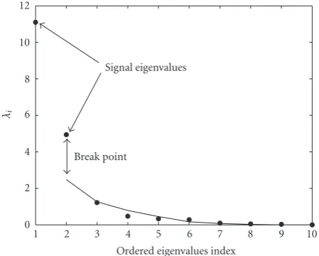
1 2 3 4 5 6 7 8 9 10
Ordered eigenvalues index 0
2 4 6 8 10 12
λi
Signal eigenvalues
Break point
Figure2: Profile of ordered noise eigenvalues in the presence of 2 sources, and 10 sensors. The ordered profile of the observed eigen-value is seen to break from the noise eigeneigen-value distribution, when there are sources present.
candidate noise eigenvalues is compatible with the theoret-ical noise eigenvalue profile. The main idea of the test is to detect the eigenvalue index at which a break occurs between the profile of the observed eigenvalues and the theoretical noise eigenvalue profile provided by the exponential model.
Figure 2shows how a break point appears between the signal
eigenvalues and the theoretical noise eigenvalue profile, while the observed noise eigenvalues are seen to fit the theoretical profile.
Firstly, an eigen-decomposition of the sample covariance matrix is performed and the resulting eigenvaluesλ1,. . .,λM, which we call the observed eigenvalues, are arranged in or-der of decreasing size. Beginning with the smallest observed eigenvalueλM, this is assumed to be a noise eigenvalue, giving the initial candidate noise subspace dimensionP=1. Then usingλM,P = 1, and the prediction equation (32) we find the next eigenvalue of the theoretical noise eigenvalue profile
λM−1:
λM−P=(P+ 1)JP+1σ2, withJP+1=
1−rP+1,N 1− rP+1,N
P+1,
σ2= 1
P+ 1 P
i=0 λM−i.
(32)
Now taking bothλM andλM−1 to be noise eigenvalues, corresponding to a candidate noise subspace dimensionP=
2, (32) is applied again to predictλM−2.
We define the following two hypotheses:
HP+1:λM−Pis a noise eigenvalue,
HP+1:λM−Pis a signal eigenvalue.
(33)
Then, starting with the smallest eigenvalue pair (that are not equal)λM−1andλM−1, the relative distance between each of the theoretical noise eigenvalues and the corresponding observed eigenvalue is found, and compared to the threshold found for that eigenvalue index, (34) and (35),
HP+1:
λM−P−λM−P λM−P
≤ηP, (34)
HP+1:
λM−P−λM−P λM−P
> ηP. (35)
If the relative difference between the theoretical noise eigen-value and the observed eigeneigen-value is less than (or equal to) the corresponding threshold, the observed eigenvalue matches the theoretical noise-only eigenvalue profile, and so it is deemed to be a noise eigenvalue, which is the case shown by (34).
We then compare the next eigenvaluesλM−2andλM−2in the same manner. This process continues until we find a pair of eigenvalues,λM−P andλM−P whose relative difference is greater than the corresponding threshold, as shown in (35). When this happens the observed eigenvalue is taken to cor-respond to a signal eigenvalue and so the test stops here. The estimated dimension of the noise subspacePis the valueP where the test stops, that is, when the hypothesis given in (35) is chosen over that in (34). The estimated model order is then given byd=M−P.
Note on the complexity
The proposed EFT method requires calculation of the sam-ple correlation matrix for each set of observations. An eigen-value decomposition of this matrix must then be performed and the smallest of the observed eigenvalues is used to pre-dict the theoretical noise-only eigenvalue profile. The com-putational cost of the EFT method is of the same order as those of the AIC and MDL tests. Compared to the methods proposed in [9,23] the computational complexity of the pro-posed algorithm is much lower due to the fact that both these algorithms rely on initially finding a maximum like-lihood estimate of the direction of arrival for each proposed number of sources. This estimation step greatly increases the computational complexity and necessitates the introduction of computational cost reduction techniques. Moreover, the PDL proposed in [23] requires the calculation of the sample covariance matrix and its eigen-decomposition at each indi-vidual snapshot.
4.2. Computation of thresholds
The comparison thresholds are closely related to the statis-tical distribution of the prediction error and are determined
to respect a preset probability of false alarmPf a. ThePf ais the probability of the method mistakenly determining that a source is present, and is defined as
Pf a=Pr d > d0|d=d0
ford0=0, 1, 2,. . .,M−1. (36)
For the noise-only cased=0, and the expression forPf acan be decomposed as follows:
Pf a=Pr d >0|d=0
=
M−1
i=1
Pr d=i|d=0=
M−1
p=1 P(p)f a,
(37)
whereP(P)f a =Pr[d=M−P |d=0] is the contribution of Pth step to the total false alarm.
Reexpressing (34) and (35) we get
HP+1:Q(P)= λM−P
M i=M−Pλi
≤ ηp+ 1
JP+1,
HP+1:Q(P)= λM−P
M i=M−Pλi
> ηp+ 1
JP+1,
(38)
resulting in the following expression for P(P)f a in the noise-only situation:
P(P)f a =Pr
Q(P)> ηP+ 1
JP+1|d=0
. (39)
Then, denoting the distribution ofQ(P) ashp(q) the thresh-oldηPis defined by the following integral equation:
P(Mf a−P)= !+∞
JP+1(ηP+1)
hP(q)dq. (40)
Solution of this equation in order to find ηP is reliant on knowledge of the distributionhP(q). ForP = M andP = M−1 the distribution is known as given in [8], but is un-usable in our application. To our knowledge, this statistical distribution is not known for other values ofP. Hence, nu-merical methods must instead be used in order to solve for ηP.
4.3. Threshold determination by Monte Carlo methods
UsingI = P(Mf a−P) for the sake of notational simplicity, we rewrite equation (40) as
I=
!
Dp λ1,. . .,λM M
i=1 dλi=E
1D, (41)
whereDis the domain of integration defined as follows: D="0< λM <· · ·< λ1<∞ |Q(P)> JP+1 ηP+ 1
# ,
(42)
0 1 2 3 4 5 6
η1
10 3
10 2
10 1
100
Pfa
(a)η1
0 0.5 1 1.5 2 2.5 3
η2
10 5
10 4
10 3
10 2
10 1
100
Pfa
(b)η2
0 0.2 0.4 0.6 0.8 1 1.2 1.4 1.6 1.8
η3
10 6
10 5
10 4
10 3
10 2
10 1
100
Pfa
(c)η3
0 0.1 0.2 0.3 0.4 0.5 0.6 0.7 0.8
η4
10 6
10 5
10 4
10 3
10 2
10 1
100
Pfa
(d)η4
Figure3: Thresholds computation forM=5 andN=10.
(i) generation of qnoise-only sample correlation matri-ces, whereqis the number of the Monte Carlo trials to be run;
(ii) computation of the ordered eigenvalues for each of theseqmatrices: (λ1,j,. . .,λM,j) 1≤j≤q;
(iii) estimation ofIbyI=(1/q)qj=11D(λ1,j,. . .,λM,j). As thePf ais usually very small,qmust be statistically de-termined in order to obtain a predefined precision for the es-timation ofI. Because of the central limit theorem,Ifollows a Gaussian law. Consequently, denoting the standard devia-tion ofIasσ, we can say Pr[(√q/σ)|I−I|< 1.96] =0.95, where Pr[x < y] is the probability that x < y. Then, as σ2=E[(1
D(·))2]−I2=I−I2≈I, we obtainσ=√I.
Application
For M = 5 sensors and a false alarm probability of 1%, identically distributed over theM−1 steps of the test,I =
P(Mf a−P)=0.01/4=0.0025 and 1≤P≤4. With a probability
of 95%,Iis estimated with an accuracy of 10% ifq=160000.
InFigure 3we have plotted theP(Mf a−P)versusηp. From this,
ηPis selected for eachPand for a givenPf a.
5. PERFORMANCE AND COMPARISON WITH CLASSICAL TESTS
In order to evaluate the test performance in white Gaussian complex noise, computed simulations have been performed with a uniform linear array of five omnidirectional sensors. The distance between adjacent sensors is half a wavelength. The number of snapshots isN =6. All the simulations have been performed with 1000 Monte Carlo simulations. Two sources of the same power impinge on the array at−10◦and +10◦. The SNR is defined as
SNR=10·log10
σ2 s σ2
, (43)
whereσ2
20 15 10 5 0 5 10 15 20 SNR (dB)
0 0.1 0.2 0.3 0.4 0.5 0.6 0.7
P
robabilit
y
o
f
false
alar
m
Pfa
AIC MDL PDL
EFT MDLB
Figure4: Comparison of the probability of false alarm for the EFT (predefinedPf a = 10%), the MDL, the AIC, the PDL, and the
MDLB.
20 15 10 5 0 5 10 15 20
SNR (dB) 0
0.1 0.2 0.3 0.4 0.5 0.6 0.7 0.8 0.9 1
P
robabilit
y
o
f
d
et
ection
AIC MDL PDL
EFT MDLB
Figure5: Probability of detection for the EFT (predefinedPf a =
10%), the MDL, the AIC, the PDL, and the MDLB.
For various SNR, all the criteria, AIC, MDL, EFT, PDL, MDLB are applied. The EFT test has firstly been designed for aPf a =10%. In such a configuration, the thresholds of the EFT test areη1 = 26.3990,η2 = 3.6367,η3 = 1.2383, andη4=0.6336. InFigure 4we have reported the probabil-ity of false alarm versus SNR for AIC, MDL, EFT, PDL, and MDLB. As expected thePf a of EFT is 10% and we observe that the uncontrolledPf aof other tests is significantly higher, except for the MDLB which is about 10% when the SNR is lower than−4 dB. InFigure 5we have reported the proba-bility of correct detection versus SNR for the same tests. We observe that only the EFT and MDLB tests give good results
20 15 10 5 0 5 10 15 20
SNR (dB) 0
0.1 0.2 0.3 0.4 0.5 0.6 0.7
P
robabilit
y
o
f
false
alar
m
Pfa
AIC MDL PDL
EFT MDLB
Figure6: Comparison of the probability of false alarm for the EFT (predefinedPf a=1%), the MDL, the AIC, the PDL, and the MDLB.
20 15 10 5 0 5 10 15 20
SNR (dB) 0
0.1 0.2 0.3 0.4 0.5 0.6 0.7 0.8 0.9 1
P
robabilit
y
o
f
d
et
ection
AIC MDL PDL
EFT MDLB
Figure7: Probability of detection for the EFT (predefinedPf a =
1%), the MDL, the AIC, the PDL, and the MDLB.
both in terms of probability of correct detection and prob-ability of false alarm. When the SNR is lower than 5 dB, the MDLB gives the best probability of detection and acceptable results for the probability of false alarm, but requires an im-portant computational complexity. When the SNR is greater than 5 dB, the EFT outperforms all the other tests in terms of Pdwith aPf astill lower than 10%.
than the classical tests in terms of correct probability of de-tectionPdfor SNR higher than 7 dB.
We can note that thePd of classical tests has drastically decreased when the noise eigenvalues are not closely clus-tered.
6. CONCLUSION
We have proposed a new test for model order selection based on the geometrical profile of noise-only eigenvalues. We have shown that noise eigenvalues for white Gaussian noise fit an exponential law whose parameters have been predicted. Contrary to traditional algorithms, this test performs well when there is a small number of snapshots used for the es-timation of the correlation matrix. Another important ad-vantage over classical tests is that the false alarm probability can be adjusted by a predetermined threshold. Moreover, the computational cost of the EFT method is of the same order as those of the AIC and MDL.
ACKNOWLEDGMENTS
The authors would like to thank the anonymous reviewers for their helpful suggestions that considerably improved the quality of the paper. This work has been partly funded by the European Network of Excellence NEWCOM.
REFERENCES
[1] Y. Q. Yin and P. R. Krishnaiah, “On some nonparametric methods for detection of the number of signals,”IEEE Transac-tions on Acoustics, Speech, and Signal Processing, vol. 35, no. 11, pp. 1533–1538, 1987.
[2] L. L. Scharf and D. W. Tufts, “Rank reduction for modeling stationary signals,”IEEE Transactions on Acoustics, Speech, and Signal Processing, vol. 35, no. 3, pp. 350–355, 1987.
[3] T. W. Anderson, “Asymptotic theory for principal component analysis,”Annals of Mathematical Statistics, vol. 34, pp. 122– 148, 1963.
[4] A. T. James, “Test of equality of latent roots of the covariance matrix,”Journal of Multivariate Analysis, pp. 205–218, 1969. [5] W. Chen, K. M. Wong, and J. Reilly, “Detection of the
num-ber of signals: a predicted eigen-threshold approach,” IEEE Transactions on Signal Processing, vol. 39, no. 5, pp. 1088–1098, 1991.
[6] P. Stoica and Y. Sel´en, “Model-order selection: a review of in-formation criterion rules,”IEEE Signal Processing Magazine, vol. 21, no. 4, pp. 36–47, 2004.
[7] H. Akaike, “A new look at the statistical model identification,” IEEE Transactions on Automatic Control, vol. 19, no. 6, pp. 716–723, 1974.
[8] J. Rissanen, “Modeling by shortest data description length,” Automatica, vol. 14, no. 5, pp. 465–471, 1978.
[9] M. Wax and T. Kailath, “Detection of signals by information theoretic criteria,”IEEE Transactions on Acoustics, Speech, and Signal Processing, vol. 33, no. 2, pp. 387–392, 1985.
[10] M. Wax and I. Ziskind, “Detection of the number of coherent signals by the MDL principle,”IEEE Transactions on Acoustics,
Speech, and Signal Processing, vol. 37, no. 8, pp. 1190–1196, 1989.
[11] M. Kaveh, H. Wang, and H. Hung, “On the theoretical per-formance of a class of estimators of the number of narrow-band sources,”IEEE Transactions on Acoustics, Speech, and Sig-nal Processing, vol. 35, no. 9, pp. 1350–1352, 1987.
[12] K. M. Wong, Q.-T. Zhang, J. Reilly, and P. Yip, “On informa-tion theoretic criteria for determining the number of signals in high resolution array processing,”IEEE Transactions on Acous-tics, Speech, and Signal Processing, vol. 38, no. 11, pp. 1959– 1971, 1990.
[13] Q. Wu and D. Fuhrmann, “A parametric method for deter-mining the number of signals in narrow-band direction find-ing,”IEEE Transactions on Signal Processing, vol. 39, no. 8, pp. 1848–1857, 1991.
[14] P. M. Djuri´c, “Model selection based on asymptotic Bayes the-ory,” inProceedings of the 7th IEEE SP Workshop on Statistical Signal and Array Processing, pp. 7–10, Quebec City, Quebec, Canada, June 1994.
[15] W. B. Bishop and P. M. Djuri´c, “Model order selection of damped sinusoids in noise by predictive densities,” IEEE Transactions on Signal Processing, vol. 44, no. 3, pp. 611–619, 1996.
[16] H. L. Van Trees,Optimum Array Processing, vol. 4 ofDetection, Estimation and Modulation Theory, John Wiley & Sons, New York, NY, USA, 2002.
[17] A. Di, “Multiple source location - a matrix decomposition approach,”IEEE Transactions on Acoustics, Speech, and Signal Processing, vol. 33, no. 5, pp. 1086–1091, 1985.
[18] H.-T. Wu, J.-F. Yang, and F.-K. Chen, “Source number estima-tors using transformed Gerschgorin radii,”IEEE Transactions on Signal Processing, vol. 43, no. 6, pp. 1325–1333, 1995. [19] A. P. Liavas and P. A. Regalia, “On the behavior of information
theoretic criteria for model order selection,”IEEE Transactions on Signal Processing, vol. 49, no. 8, pp. 1689–1695, 2001. [20] A. Quinlan, J.-P. Barbot, and P. Larzabal, “Automatic
deter-mination of the number of targets present when using the time reversal operator,”The Journal of the Acoustical Society of America, vol. 119, no. 4, pp. 2220–2225, 2006.
[21] M. Tanter, J.-L. Thomas, and M. Fink, “Time reversal and the inverse filter,”The Journal of the Acoustical Society of America, vol. 108, no. 1, pp. 223–234, 2000.
[22] J. Grouffaud, P. Larzabal, and H. Clergeot, “Some properties of ordered eigenvalues of a Wishart matrix: application in detec-tion test and model order selecdetec-tion,” inProceedings of the IEEE International Conference on Acoustics, Speech and Signal Pro-cessing (ICASSP ’96), vol. 5, pp. 2463–2466, Atlanta, Ga, USA, May 1996.
[23] S. Valaee and P. Kabal, “An information theoretic approach to source enumeration in array signal processing,”IEEE Transac-tions on Signal Processing, vol. 52, no. 5, pp. 1171–1178, 2004. [24] B. Champagne, “Adaptive eigendecomposition of data
covari-ance matrices based on first-order perturbations,”IEEE Trans-actions on Signal Processing, vol. 42, no. 10, pp. 2758–2770, 1994.
[26] N. L. Johnson and S. Kotz,Distributions in Statistics: Contin-uous Multivariate Distributions, chapter 38-39, John Wiley & Sons, New York, NY, USA, 1972.
[27] P. R. Krishnaiah and F. J. Schurmann, “On the evaluation of some distribution that arise in simultaneous tests of the equal-ity of the latents roots of the covariance matrix,”Journal of Multivariate Analysis, vol. 4, pp. 265–282, 1974.
Angela Quinlan studied engineering in Trinity College Dublin, Ireland, and re-ceived her B.S. degree in electronic engi-neering in June 2002. In October 2002, she began her Ph.D. in the Department of Elec-tronics in Trinity College. From 2004 to 2005, she completed a year working with the Signal Processing and Information Team at the SATIE Laboratory at the ´Ecole Normale Sup´erieure de Cachan. She will defend her
Ph.D. thesis in June 2006. Her research interests include statistical signal and array processing, audio source localization, audio time reversal focusing, and estimator performance bounds.
Jean-Pierre Barbot was born in Tours, France, in 1964. He received the Agrega-tion degree in electrical engineering from the ´Ecole Normale Sup´erieure de Cachan, France, in 1988. In 1995, he received the Ph.D. degree from the University Paris-Sud, France. From 1990 to 1994, he worked in the CNET (France Telecom), Paris, France, where he was involved in indoor propa-gation studies for mobile communications.
From 1994 to 1996, he was a teacher in the Electrical Engineer-ing Department of the Institut Universitaire of Technologie of Velizy, University of Versailles Saint-Quentin, France, and worked in the CETP Laboratory, UMR-8639 CNRS, University of Ver-sailles Saint-Quentin, France, on propagation studies. In 1996, he joined the Electrical Engineering Department of the ´Ecole Normale Sup´erieure de Cachan, France, as an Associate Professor. He teaches electronics, microwaves, signal processing, and numerical commu-nications. He is a Member of the Signal Processing Team of SATIE Laboratory, UMR CNRS, ´Ecole Normale Sup´erieure de Cachan, France. His current research interest is in the field of estimation applied to numerical communications and radar. He is a Member of the European Network of Excellence NEWCOM.
Pascal Larzabal was born in the Basque country in the south of France in 1962. He received the Agregation degree in elec-trical engineering and the Ph.D. degree from ´Ecole Normale Sup´erieure de Cachan, France, in 1988 and 1992, respectively, and the Habilitation `a Diriger les Recherches degree from ´Ecole Normale Sup´erieure de Cachan, France, in 1998. He is now a Pro-fessor at the Institut Universitaire de
Tech-nologie de Cachan, University of Paris-Sud, France, where he is the Head of the Electrical Engineering Department. He teaches elec-tronics, signal processing and control. He is the Head of the Sig-nal Processing Team of SATIE Laboratory, UMR CNRS, ´Ecole Nor-male Sup´erieure de Cachan, where his research concerns estima-tion in array processing and spectral analysis for communicaestima-tions and radar. He is a Member of the European Network of Excellence NEWCOM.
Martin Haardt has been a Full Profes-sor and Head of the Communications Re-search Laboratory at Ilmenau University of Technology, Germany, since 2001. Af-ter studying electrical engineering at the Ruhr-University Bochum, Germany, and at Purdue University, USA, he received his Diplom-Ingenieur (M.S.) degree from the Ruhr-University Bochum in 1991 and his Doktor-Ingenieur (Ph.D.) degree from