Multi-dimensional model order selection

(1)

R E S E A R C H

Open Access

Multi-dimensional model order selection

João Paulo Carvalho Lustosa da Costa

1*

, Florian Roemer

2

, Martin Haardt

2

and Rafael Timóteo de Sousa Jr

1

Abstract

Multi-dimensional model order selection (MOS) techniques achieve an improved accuracy, reliability, and robustness, since they consider all dimensions jointly during the estimation of parameters. Additionally, from fundamental identifiability results of multi-dimensional decompositions, it is known that the number of main components can be larger when compared to matrix-based decompositions. In this article, we show how to use tensor calculus to extend matrix-based MOS schemes and we also present our proposed multi-dimensional model order selection scheme based on the closed-form PARAFAC algorithm, which is only applicable to

multi-dimensional data. In general, as shown by means of simulations, the Probability of correct Detection (PoD) of our proposed multi-dimensional MOS schemes is much better than the PoD of matrix-based schemes.

Introduction

In the literature, matrix array signal processing techni-ques are extensively used in a variety of applications including radar, mobile communications, sonar, and seismology. To estimate geometrical/physical parameters such as direction of arrival, direction of departure, time of direction of arrival, and Doppler frequency, the first step is to estimate the model order, i.e., the number of signal components.

By taking into account only one dimension, the pro-blem is seen from just one perspective, i.e., one projec-tion. Consequently, parameters cannot be estimated properly for certain scenarios. To handle that, multi-dimensional array signal processing, which considers several dimensions, is studied. These dimensions can correspond to time, frequency, or polarization, but also spatial dimensions such as one- or two-dimensional arrays at the transmitter and the receiver. With multi-dimensional array signal processing, it is possible to esti-mate parameters using all the dimensions jointly, even if they are not resolvable for each dimension separately. Moreover, by considering all dimensions jointly, the accuracy, reliability, and robustness can be improved. Another important advantage of using multi-dimen-sional data, also known as tensors, is the identifiability, since with tensors the typical rank can be much higher than using matrices. Here, we focus particularly on the

development of techniques for the estimation of the model order.

The estimation of the model order, also known as the number of principal components, has been investigated in several science fields, and usually model order selec-tion schemes are proposed only for specific scenarios in the literature. Therefore, as a first important contribu-tion, we have proposed in [1,2] the one-dimensional model order selection scheme called Modified Exponen-tial Fitting Test (M-EFT), which outperforms all the other schemes for scenarios involving white Gaussian noise. Additionally, we have proposed in [1,2] improved versions of the Akaike’s Information Criterion (AIC) and Minimum Description Length (MDL).

As reviewed in this article, the multi-dimensional structure of the data can be taken into account to improve further the estimation of the model order. As an example of such improvement, we show our

pro-posed R-dimensional Exponential Fitting Test (R-D

EFT) for multi-dimensional applications, where the noise is additive white Gaussian. TheR-D EFT success-fully outperforms the M-EFT confirming that even the technique with the best performance can be improved by taking into account the multi-dimensional structure of the data [1,3,4]. In addition, we also extend our modified versions of AIC and MDL to their respective multi-dimensional versionsR-D AIC andR-D MDL. For scenarios with colored noise, we present our proposed multi-dimensional model order selection technique called closed-form PARAFAC-based model order selection (CFP-MOS) scheme [3,5].

* Correspondence: [email protected]

1

University of Brasília, Electrical Engineering Department, P.O. Box 4386, 70910-900 Brasília, Brazil

Full list of author information is available at the end of the article

(2)

The remainder of this article is organized as follows. After reviewing the notation in second section, the data model is presented in third section. Then theR -dimen-sional exponential fitting test (R-D EFT) and closed-form PARAFAC-based model order selection (CFP-MOS) scheme are reviewed in fourth section. The simu-lation results in fifth section confirm the improved per-formance of R-D EFT and CFP-MOS. Conclusions are drawn finally.

Tensor and matrix notation

In order to facilitate the distinction between scalars, matrices, and tensors, the following notation is used: Scalars are denoted as italic letters (a,b, ...,A, B, ...,a, b, ...), column vectors as lower-case bold-face letters (a,

b, ...), matrices as bold-face capitals (A,B, ...), and ten-sors are written as bold-face calligraphic letters (A,B,. . .). Lower-order parts are consistently named: the (i, j)-element of the matrix Ais denoted as ai,jand

the (i, j, k)-element of a third order tensorX asxi,j,k.

The n-mode vectors of a tensor are obtained by varying thenth index within its range (1, 2, ..., In) and keeping

all the other indices fixed. We use the superscripts T, H, -1, +, and* for transposition, Hermitian

transposi-tion, matrix inversion, the Moore-Penrose pseudo inverse of matrices, and complex conjugation, respec-tively. Moreover the Khatri-Rao product (columnwise Kronecker product) is denoted byA◊B.

The tensor operations we use are consistent with [6]: Ther-mode productof a tensor_A_∈_CI1×I2×···×IRand a matrix U∈CJr×Iralong the rth mode is denoted as A×rU∈CI1×I2···×Jr···×IR. It is obtained by multiplying all

r-mode vectors of A from the left-hand side by the

matrix U. A certain r-mode vector of a tensor is

obtained by fixing the rth index and by varying all the other indices.

The higher-order SVD (HOSVD) of a tensor

A∈CI1×I2×···×IRis given by

A=S×1U1×2U2· · · ×RUR, (1)

where_S_∈_CI1×I2×···×IRis the core-tensor which satis-fies the all-orthogonality conditions [6] andUr∈CIr×Ir,r

= 1, 2, ...,Rare the unitary matrices ofr-mode singular vectors.

Finally, ther-mode unfolding of a tensor_A is symbo-lized by[A](r)∈CIr×(I1I2...Ir−1Ir+1...IR), i.e., it represents the

matrix ofr-mode vectors of the tensor_A. The order of the columns is chosen in accordance with [6].

Data model

To validate the general applicability of our proposed schemes, we adopt the PARAFAC data model below

x0(m1,m2,. . .,mR+1) =

d

n=1

fn(1)(m1)·fn(2)(m2). . .fn(R+1)(mR+1), (2)

where fn(r)(mr)is the mrth element of thenth factor of

therth mode formr = 1, ...,Mrandr= 1, 2, ...,R,R+1.

TheMR+1 can be alternatively represented byN, which

stands for the number of snapshots.

By defining the vectors

f(_nr)=

fn(r)(1)fn(r)(2). . .fn(r)(Mr) T

and using the outer

product operator∘, another possible representation of (2) is given by

X0=

d

n=1

f(1)_n ◦f(2)_n ◦ · · · ◦f(_nR+1), (3)

where_X₀_∈_CM1×M2···×MR×MR+1is composed of the sum

ofdrank one tensors. Therefore, the tensor rank ofX0

coincides with the model orderd.

For applications, where the multi-dimensional data obeys a PARAFAC decomposition, it is important to estimate the factors of the tensorX0, which are defined

as F(r)=

f(₁r),. . .,f(_dr)

∈CMr×d_{, and we assume that the} rank of eachF(r)is equal to min(Mr,d). This definition

of the factor matrices allows us to rewrite (3) according to the notation proposed in [7]

X0=IR+1,d×1F(1)×2F(2)· · · ×R+1F(R+1), (4)

where ×ris ther-mode product defined in Section 2,

and the tensor IR+1,drepresents theR-dimensional

iden-tity tensor of sized×d... × d, whose elements are equal to one when the indices i1 = i2 ... = iR+1 and zero

otherwise.

In practice, the data is contaminated by noise, which we represent by the following data model

X =IR+1,d×1F(1)×2F(2)· · · ×R+1F(R+1)+N, (5)

where_N _∈_CM1×M2···×MR+1is the additive noise tensor,

whose elements are i.i.d. zero-mean circularly symmetric complex Gaussian (ZMCSCG) random variables. Thereby, the tensor rank is different fromdand usually it assumes extremely large values as shown in [8]. Hence, the problem we are solving can therefore be stated in the following fashion: given a noisy measurement tensor_X,

we desire to estimate the model order d. Note that

according to Comon [8], the typical rank of_X is much

bigger than any of the dimensionsMrforr= 1, ...,R+ 1.

The objective of the PARAFAC decomposition is to compute the estimated factors_F_ˆ(r)_{such that}

X ≈IR+1,d×1Fˆ

(1)

×2Fˆ(2)· · · ×RFˆ

(R+1)

(3)

Since_F_ˆ(r)

∈CMr×done requirement to apply the PAR-AFAC decomposition is to estimated.

We evaluate the performance of the model order selection scheme in the presence of colored noise, which is given by replacing the white Gaussian white

noise tensor _N by the colored Gaussian noise tensor

N(c)_{in (5). Note that the data model used in this article}

is simply a linear superposition of rank-one components superimposed by additive noise.

Particularly, for multi-dimensional data, the colored noise with a Kronecker structure is present in several applications. For example, in EEG applications [9], the noise is correlated in both space and time dimensions, and it has been shown that a model of the noise com-bining these two correlation matrices using the Kro-necker product can fit noise measurements. Moreover, for MIMO systems the noise covariance matrix is often assumed to be the Kronecker product of the temporal and spatial correlation matrices [10].

The multi-dimensional colored noise, which is assumed to have a Kronecker correlation structure, can be written as

N(c)

(R+1)= [N](R+1)·(L1⊗L2⊗ · · · ⊗LR) T

, (7)

where ⊗represents the Kronecker product. We can

also rewrite (7) using the n-mode products in the fol-lowing fashion

N(c)₌_N_×1_L_1×2_L

2· · · ×RLR, (8)

where _N _∈_CM1×M2···×MR×MR+1is a tensor with

uncor-related ZMCSCG elements with variance σ2

n, and

Li∈CMi×Miis the correlation factor of theith dimension

of the colored noise tensor. The noise covariance matrix in theith mode is defined as

E

N(c)

(i)·

N(c)H (i)

=α·Wi=α·Li·LHi , (9)

where a is a normalization constant, such that

tr(Li·LHi ) =Mi. The equivalence between (7), (8), and

(9) is shown in [11].

To simplify the notation, let us define M=R_r₌₁Mr.

For ther-mode unfolding we compute the sample

cov-ariance matrix as

ˆ

R(_xxr)= Mr

M[X](r)·[X]

H (r)∈C

MrxMr_. ₍₁₀₎

The eigenvalues of these r-mode sample covariance

matrices play a major role in the model order estimation step. Let us denote theith eigenvalue of the sample cov-ariance matrix of the r-mode unfolding as _λ(_ir). Notice

that Rˆ(_xxr)possesses Mr eigenvalues, which we order in

such a way that _λ(₁r)_≥_λ₂(r) _{≥ · · ·}_λ(_Mr)

r. The eigenvalues may be computed from the HOSVD of the measure-ment tensor

X =S×1U1×2U2· · · ×R+1UR+1 (11)

as

diagλ(₁r),λ₂(r),. . .,λ(_Mr)_r = Mr

M[S](r)·[S]

H

(r). (12)

Note that the eigenvalues _λ(_ir) are related to the

r-mode singular values _σ_i(r) of X through

λ(r)

i =

Mr

M

σ(r)

i

2

. The r-mode singular values _σ_i(r)can

also be computed via the SVD of ther-mode unfolding

X as follows

[X](r)=Ur·r·VHr, (13)

where Ur∈CMr×Mr and

Vr∈C

M

Mr

×M

Mr are unitary

matrices, and

r∈C Mr×

M

Mr is a diagonal matrix, which

contains the singular values_σ_i(r)on the main diagonal.

Multi-dimensional model order selection schemes

In this section, the multi-dimensional model order selection schemes are proposed based on the global

eigenvalues, the R-D subspace, or tensor-based data

model. First, we show the proposed definition of the global eigenvalues together with the presentation of the

proposed R-D EFT. Then, we summarize our

multi-dimensional extension of AIC and MDL. Besides the global eigenvalues-based schemes, we also propose a tensor data-based multi-dimensional model order selec-tion scheme. Followed by the closed-form PARAFAC-based model order selection scheme is proposed for white and also colored noise scenarios. For data sampled on a grid and an array with centro-symmetric symme-tries, we show how to improve the performance of model order selection schemes for such data by incor-porating forward-backward averaging (FBA).

R-D exponential fitting test (R-D EFT)

The global eigenvalues are based on ther-mode eigen-values represented by _λ(_ir)for r = 1, ...,Rand for i= 1, ..., Mr. To obtain the r-mode eigenvalues, there are two

ways. The first way shown in (10) is possible via the EVD of eachr-mode sample covariance matrix, and the second way in (12) is given via an HOSVD.

(4)

curve. Therefore, by applying the exponential approxi-mation for everyr-mode, we obtain that

E{λ(_ir)}= E{λ₁(r)} ·q(αr,βr)i−1, (14)

where αr= min

Mr,

M

Mr

, βr= max

Mr,

M

Mr

, i =

1,2, ...,Mrandr = 1, 2, ...,R+ 1. The rate of the

expo-nential profileq(ar,br) is defined as

q(α,β) = exp ⎧ ⎨ ⎩−

30

α2_{+ 2}−

900 (α2_{+ 2)}2−

720α β(α4₊_α2₋₂₎

⎫ ⎬ ⎭, (15)

wherea= min (M,N) and b= max (M,N). Note that (15) of the M-EFT is an extension of the EFT expression in [12,13].

In order to be even more precise in the computation ofq, the following polynomial can be solved

(C−1)·qα+1+ (C+ 1)·qα−(C+ 1)·q+ 1−C= 0. (16)

Although from (16) a + 1 solutions are possible, we

select only theq that belongs to the interval (0, 1). For

M ≤N(15) is equal to the q of the EFT [12,13], which means that the PoD of the EFT and the PoD of the M-EFT are the same forM <N. Consequently, the M-EFT automatically inherits from the EFT the property that it outperforms the other matrix-based MOS techniques in the literature forM ≤Nin the presence of white Gaus-sian noise as shown in [2].

For the sake of simplicity, let us first assume that M1

=M2 = ... = MR. Then we can defineglobal eigenvalues

as being [1]

λ(G)

i =λ

(1)

i ·λ

(2)

i . . .·λ

(R+1)

i . (17)

Therefore, based on (14), it is straightforward that the noise global eigenvalues also follow an exponential pro-file, since

Eλ(G)_i = Eλ(G)₁ ·q(α1,β1)·. . .·q(αR,βR) i−1

, (18)

wherei= 1, ...,MR+1.

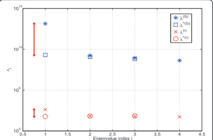
In Figure 1, we show an example of the exponential pro-file property that is assumed for the noise eigenvalues. This exponential profile approximates the distribution of the noise eigenvalues and the distribution of the global noise eigenvalues. The exemplified data in Figure 1 have the model order equal to one, since the first eigenvalue does not fit the exponential profile. To estimate the model order, the noise eigenvalue profile gets predicted based on the exponential profile assumption starting from the smal-lest noise eigenvalue. When a significant gap is detected compared to this predicted exponential profile, the model order, i.e., the smallest signal eigenvalue, is found.

The product across modes increases the gap between the predicted and the actual eigenvalues as shown in Figure 1. We compare the gap between the actual eigen-values and the predicted eigeneigen-values in therth mode to the gap between the actual global eigenvalues and the predicted global eigenvalues. Here, we consider thatX0

is a rank one tensor, and noise is added according to (5)

Then, in this case, d = 1. For the first gap, we have

λ(r)

i − ˆλ

(r)

i = 2.4×102, while for the second one, we

have _λ(G)₁ _{− ˆ}_λ(G)₁ = 2.4×1012. Therefore, the break in

the profile is easier to detect via global eigenvalues than using only one mode eigenvalues

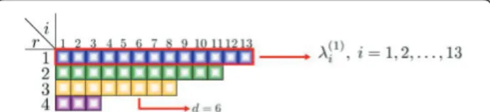
Since all tensor dimensions may be not necessarily equal to each other, without loss of generality, let us consider the case in whichM1≥M2≥...≥MR+1. In Figures 2, 3,

and 4, we have sets of eigenvalues obtained from each

r-mode of a tensor with sizesM1= 13,M2= 11,M3= 8

andM4 = 3. The indexiindicates the position of the

eigenvalues in eachrth eigenvalues set.

We start by estimating _dˆ with a certain eigenvalue-based model order selection method considering the first unfolding only, which in the example in Figure 2 has a size M1= 13. If dˆ<M₂, we could have taken

advantage of the second mode as well. Therefore, we compute the global eigenvalues_λ(G)_i as in (17) for 1 ≤ i

≤ M2, thus discarding the M1 - M2 last eigenvalues of

the first mode. We can obtain a new estimate_dˆ. As illu-strated in Figure 3, we utilize only the firstM2 highest

eigenvalues of the first and of the second modes to esti-mate the model order. If _dˆ_<_M₃we could continue in the same fashion, by computing the global eigenvalues considering the first three modes. In the example in Fig-ure 4, since the model order is equal to 6, which is greater than M4, the sequential definition algorithm of

0.5 1 1.5 2 2.5 3 3.5 4 4.5 100

105

1010

1015

Eigenvalue index i

λi

λ(G) λ^(G) λ(r) λ^(r)

Figure 1Comparison between the global eigenvalues profile and theR-mode eigenvalues profile for a scenario with array sizeM1= 4,M2= 4,M3= 4,M4= 4,M5= 4,d= 1 and SNR =

(5)

the global eigenvalues stops using the three first modes. Clearly, the full potential of the proposed method can be achieved when all modes are used to compute the global eigenvalues. This happens when_dˆ_<_M_R₊₁, so that

λ(G)

i can be computed for 1≤i≤MR+1.

Note that using the global eigenvalues, the assump-tions of M-EFT, that the noise eigenvalues can be approximated by an exponential profile, and the assumptions of AIC and MDL, that the noise eigenva-lues are constant, still hold. Moreover, the maximum model order is equal tomax_r Mr, for r= 1, ...,R.

The R-D EFT is an extended version of the M-EFT

operating on the_λ(G)_i . Therefore,

1) It exploits the fact that the noise global eigenva-lues still exhibit an exponential profile;

2) The increase of the threshold between the actual signal global eigenvalue and the predicted noise glo-bal eigenvalue leads to a significant improvements in the performance;

3) It is applicable to arrays of arbitrary size and dimension through the sequential definition of the global eigenvalues as long as the data is arranged on a multi-dimensional grid.

To derive the proposed multi-dimensional extension

of the M-EFT algorithm, namely theR-D EFT, we start

by looking at anR-dimensional noise-only case. For the

R-D EFT, it is our intention to predict the noise global eigenvalues defined in (18). Eachr-mode eigenvalue can be estimated via

ˆ λ(r)

M−P= (P+ 1)·

1−q

P+ 1, M

Mr

1−q

P+ 1, M

Mr

P+1

ˆ σ(r) 2

(19)

ˆ

σ(r) 2₌ 1

P

P−1

i=0 λ(r)

M−i. (20)

Equations (19) and (20) are the same expressions as in the case of the M-EFT in [2], however, in contrast to

the M-EFT, here they are applied to each r-mode

eigenvalue.

Let us apply the definition of the global eigenvalues according to (17)

ˆ λ(G)

i =λˆ

(1)

i · ˆλ

(2)

i . . .λˆ

(R)

i , (21)

where in (18) the approximation by an exponential profile is assumed. Therefore,

ˆ

λ(G)

i =λˆ

(G) α(G)·

q

P+ 1, M

M1

·. . .·q

P+ 1, M

MR i−1

, (22)

where a(G) is the minimum ar for all the r-modes

considered in the sequential definition of the global eigenvalue. In (22),_λˆ(G)_i is a function of only the last

global eigenvalue λˆ(G)_α(G), which is the smallest global

eigenvalue and is assumed a noise eigenvalue, and of

the rates q

P+ 1, M

Mr

for all the r-modes considered

in the sequential definition. Instead of using directly (22), we use_λˆ(_Mr)₋_Paccording to (19) for all ther-modes considered in the sequential definition. Therefore, the previous eigenvalues that were already estimated as noise eigenvalues are taken into account in the predic-tion step.

Similarly to the M-EFT, using the predicted global

eigenvalue expression (21) considering white

Gaussian noise samples, we compute the global threshold coefficients_η(G)_P via the hypotheses for the tensor case

HP+1:λ(G)M−Pis a noise EV, λ(G)

M−P− ˆλ

(G)

M−P ˆ λ(G)

M−P

≤η(G)

P

¯

HP+1:λ(G)M−Pis a signal EV, λ(G)

M−P− ˆλ

(G)

M−P ˆ λ(G)

M−P

> η(G)

P .

(23)

Once all _η(G)

P are found for a certain higher order

array of sizesM1,M2, ...,MR, and for a certainPfa, then Figure 2Sequential definition of the global eigenvalues-1st

eigenvalue set.

Figure 3Sequential definition of the global eigenvalues-1st and 2nd eigenvalue sets.

(6)

the model order can be estimated by applying the following cost function

ˆ

d=α(G)−min(P) where

P∈P, if λ

(G)

M−P− ˆλ

(G)

M−P

ˆ λ(G)

M−P

> η(G)

P ,

wherea(G)is the total number of sequentially defined global eigenvalues.

R-D AIC andR-D MDL

In AIC and MDL, it is assumed that the noise eigenva-lues are all equal. Therefore, once this assumption is valid for all r-mode eigenvalues, it is straightforward that it is also valid for our global eigenvalue definition. Moreover, since we have shown in [2] that 1-D AIC and 1-D MDL are more general and superior in terms of performance than AIC and MDL, respectively, we extend 1-D AIC and 1-D MDL to the multi-dimensional form using the global eigenvalues. Note that the PoD of 1-D AIC and 1-D MDL is only greater than the PoD of AIC and MDL for cases where _MM_r >Mr, which cannot

be fulfilled for one-dimensional data.

The correspondingR-dimensional versions of 1-D AIC and 1-D MDL are obtained by first replacing the eigenva-luesRˆxxby the global eigenvaluesλ

(G)

i defined in (17).

Addi-tionally, to compute the number of free parameters for the 1-D AIC and 1-D MDL methods and theirR-D extensions, we propose to set the parameterN= max_r Mranda(G)is the total number of sequentially defined global eigenvalues similarly as we propose in [1]. Therefore, the optimization problem for theR-D AIC and R-D MDL is given by

ˆ

d= arg min

P J

(G)₍_P₎ _where

J(G)(P) =−N(α(G)−P) log

g(G)₍_P₎ a(G)₍_P₎

+p(P,N,α(G)), (24)

where_dˆ represents an estimate of the model order d, andg(G)(P) and a(G)(P) are the geometric and arithmetic means of theP smallest global eigenvalues, respectively. The penalty functions p(P,Na(G)) forR-D AIC and R-D MR-DL are given in Table 1.

Note that the R-dimensional extension described in

this section can be applied toany model order selection

scheme that is based on the profile of eigenvalues, i.e., also to the 1-D MDL and the 1-D AIC methods.

Closed-form PARAFAC-based model order selection (CFP-MOS) scheme

In this section, we present the Closed-form PARAFAC-based model order selection (CFP-MOS) technique pro-posed in [5]. The major motivation of CFP-MOS is the fact that R-D AIC,R-D MDL, andR-D EFT are applic-able only in the presence of white Gaussian noise. Therefore, it is very appealing to apply CFP-MOS, since it has a performance close toR-D EFT in the presence of white Gaussian noise, and at the same time it is also applicable in the presence of colored Gaussian noise.

According to Roemer and Haardt [14], the estimation of the factorsF(r)via the PARAFAC decomposition is transformed into a set of simultaneous diagonalization problems based on the relation between the truncated

HOSVD [6]-based low-rank approximation of_X

X ≈S[s]_×1_U[s]

1 · · · ×R+1U[s]_R₊₁

≈S[s]R_×+1

r=1rU [S]

r ,

(25)

and the PARAFAC decomposition of_X

X ≈IR+1,d×1Fˆ

(1)

· · · ×R+1Fˆ (R+1)

≈IR+1,d R+1

×

r=1rFˆ (r)

,

(26)

where _S[s] _∈_Cp1×p2×···×pR+1, _U[s]

r ∈CMr×pr, pr = min

(Mr,d), and _Fˆ(r)₌_U[s]_r ·_T_rfor a nonsingular

transforma-tion matrix Tr Î ℂd × d for all modes r∈R where

R={r|Mr≥d, r = 1,. . .R+ 1} denotes the set of

non-degenerate modes. As shown in (25) and in (26),

the operatorR×+1

r=1rdenotes a compact representation ofR

r-mode products between a tensor andR+ 1 matrices. The closed-form PARAFAC (CFP) [14] decomposition constructs two simultaneous diagonalization problems for every tuple (k,ℓ), such that k, _∈R, and k < ℓ. In order to reference each simultaneous matrix diagona-lization (SMD) problem, we define the enumerator function e(k, ℓ, i) that assigns the triple (k, ℓ, i) to a sequence of consecutive integer numbers in the range 1, 2, ..., T. Here i = 1, 2 refers to the two simultaneous matrix diagonalizations (SMD) for our specific kandℓ. Consequently, SMD (e (k, ℓ, 1), P) represents the first

SMD for a given k and ℓ, which is associated to the

simultaneous diagonalization of the matrices Srhs

k,,(n)by

T k. Initially, we consider that the candidate value of

the model orderP =d, which is the model order. Simi-larly, SMD (e (k, ℓ, 2), P) corresponds to the second

SMD for a given kand ℓ referring to the simultaneous

Table 1 Penalty functions forR-D information theoretic criteria

Approach Penalty functionp(P,N,a(G)₎

R-D AIC P · (2 ·a(G)_-_P₎

R-D MDL 1

2·P·(2·α

(7)

diagonalizations of Slhs_k_,_,(_n₎by Tℓ. Srhs_k_,_,(_n₎andSlhs_k_,_,(_n₎are defined in [14]. Note that each SMD(e(k, ℓ, i),P) yields an estimate of all factors F(r)[14,15], where r= 1, ..., R. Consequently, for each factorF(r)there areTestimates.

For instance, consider a 4-D tensor, where the third mode is degenerate, i.e., M3 <d. Then, the set R+ 1is

given by {1, 2, 4}, and the possible (k,ℓ)-tuples are (1,2), (1,4), and (2,4). Consequently, the six possible SMDs are enumerated via e(k, ℓ,i) as follows:e(1, 2, 1) = 1,e(1, 2, 2) = 2,e(1, 4, 1) = 3, e(1, 4, 2) = 4, e(2, 4, 1) = 5, and e

(2, 4, 2) = 6. In general, the total number of SMD pro-blemsTis equal to#(R−1)·[#(R)].

There are different heuristics to select the best esti-mates of each factor F(r) as shown in [14]. We define the function to compute the residuals (RESID) of the simultaneous matrix diagonalizations (SMD) as RESID (SMD(·)). For instance, we apply it toe(k,ℓ, 1)

RESID(SMD(e(k,, 1),P)) = Nmax

n=1 offT−1

k ·S

rhs

k,,(n)·Tk

2

F, (27)

and fore(k,ℓ,2)

RESID(SMD(e(k,, 2),P)) =

Nmax

n=1

offT−1·S_klhs_,_,(_n₎·T

2

F, (28)

whereNmax=

R r=1

Mr·N/(Mk·M).

Since each residual is a positive real-valued number, we can order the SMDs by the magnitude of the corre-sponding residual. For the sake of simplicity, we repre-sent the ordered sequence of SMDs to e(k, ℓ, i) by a single indexe(t)fort= 1, 2, ..., T, such that RESID(SMD (e(t),P))≤RESID(SMD(e(t+1),P)). Since in practicedis not known,P denotes a candidate value for_dˆ, which is our estimate of the model orderd. Our task is to select

P from the interval dˆmin≤P≤ ˆdmax, where dˆminis a

lower bound anddˆmaxis an upper bound for our

candi-date values. For instance, dˆminequal to 1 is used, and ˆ

dmax is chosen such that no dimension is degenerate

[14], i.e.d ≤Mr forr= 1, ...,R. We define RESID(SMD

(e(t), P)) as being the tth lowest residual of the SMD considering the number of components per factor equal toP. Based on the definition of RESID(SMD(e(t),P)), one

first direct way to estimate the model order dcan be

performed using the following properties

1) If there is no noise andP <d, then RESID(SMD(e(t),

P)) > RESID(SMD(e(t),d)), since the matrices generated are composed of mixed components as shown in [16].

2) If noise is present andP >d, then RESID(SMD(e(t),

P)) > RESID(SMD(e(t),d)), since the matrices generated with the noise components are not diagonalizable com-muting matrices. Therefore, the simultaneous diagonali-zations are not valid anymore.

Based on these properties, a first model order selection scheme can be proposed

ˆ

d= arg min

P RESID(SMD(e

(1)_,_P_)).

(29)

However, the model order selection scheme in (29) yields a Probability of correct Detection (PoD) inferior to the some MOS techniques found in the literature. Therefore, to improve the PoD of (29), we propose to exploit the redundant information provided only by the closed-form PARAFAC (CFP) [14].

Let Fˆ(_er(t))_,_Pdenote the ordered sequence of estimates for

F(r)

assuming that the model order isP. In order to

combine factors estimated in different diagonalizations processes, the permutation and scaling ambiguities should be solved. For this task, we apply the amplitude approach according to Weis et al. [15]. For the correct model order and in the absence of noise, the subspaces of F(_er(t))_,_Pshould not depend ont. Consequently, a

mea-sure for the reliability of the estimate is given by com-paring the angle between the vectors _fˆ(r)

v,e(t)_,_Pfor different

t, where ˆ_f(_v_,r_e)(t)_,_Pcorresponds to the estimate of the vth

column of F(_er(t))_,_P. Hence, this gives rise to an expression

to estimate the model order using CFP-MOS

ˆ

d= arg min

P RMSE(P) where

RMSE(P) = (P)·

Tlim

t=2

R

r=1

P

v=1

ˆ

f(vr,e)(t),P,fˆ

(r)

v,e(1),P

, (30)

where the operator∢gives the angle between two vec-tors andTlimrepresents the total number of simultaneous

matrix diagonalizations taken into account.Tlim, a design

parameter of the CFP-MOS algorithm, can be chosen between 2 andT. Similar to the Threshold Core Consis-tency Analysis (T-CORCONDIA) in [4], the CFP-MOS requires weightsΔ(P), otherwise the Probabilities of cor-rect Dectection (PoD) for different values ofdhave a sig-nificant gap from each other. Therefore, to have a fair estimation for all candidatesP, we introduce the weights Δ(P), which are calibrated in a scenario with white Gaus-sian noise, where the number of sourcesdvaries. For the calibration of weights, we use the probability of correct detection (PoD) of theR-D EFT [1,4] as a reference, since the R-D EFT achieves the best PoD in the literature even in the low SNR regime. Consequently, we propose the fol-lowing expression to obtain the calibrated weightsΔvar

var= arg min

Jvar() where

Jvar() =

dmax

P=dmin

EPoDCFP - MOSSNR ( (P))

(8)

whereE{PoDR- D EFT

SNR (P)}returns the averaged

prob-ability of correct detection over a certain predefined

SNR range using the R-D EFT for a given scenario

assuming P as the model order, dmax is defined as

being the maximum candidate value ofP, and Δvar is

the vector with the threshold coefficients for each

value of P. Note that the elements of the vector of

weights Δ vary according to a certain defined range

and interval and that the averaged PoD of the

CFP-MOS is compared to the averaged PoD of the R-D

EFT. When the cost function is minimized, then we have the desiredΔvar.

Up to this point, the CFP-MOS is applicable to sce-narios without any specific structure in the factor matrices. If the vectors f(_vr_,_e)(t)_,_P have a Vandermonde

structure, we can propose another expression. Again let

ˆ

F(er(t))_,_Pbe the estimate for therth factor matrix obtained

from SMD(e(t),P). Using the Vandermonde structure of each factor we can estimate the scalars μ(_vr_,_e)(t)_,_P

corre-sponding to the vth column of _Fˆ(r)

e(t)_,_PAs already

pro-posed previously, for the correct model order and in the absence of noise, the estimated spatial frequencies

should not depend on t. Consequently, a measure for

the reliability of the estimate is given by comparing the estimates for differentt. Hence, this gives rise to the new cost function

ˆ

d= arg min

P RMSE(P) where

RMSE(P) = (P)·

Tlim

t=2

R

r=1

P

v=1

ˆ μ(r)

v,e(t)_,_P− ˆμ (r)

v,e(1)_,_P .

(32)

Similar to the cost function in (30), to have a fair estimation for all candidatesP, we introduce the weights Δ(P), which are calculated in a similar fashion as for T-CORCONDIA Var in [4] by considering data con-taminated by white Gaussian noise.

Applying forward-backward averaging (FBA)

In many applications, the complex-valued data obeys additional symmetry relations that can be exploited to enhance resolution and accuracy. For instance, when sampling data uniformly or on centro-symmetric grids,

the corresponding r-mode subspaces are invariant

under flipping and conjugation. Such scenarios are known as having centro-symmetric symmetries. Also in such scenarios, we can incorporate FBA [17] to all model order selection schemes even with a multi-dimensional data model. First, let us present modifica-tions in the data model, which should be considered to apply the FBA. Comparing the data model of (4) to the data model to be introduced in this section, we

summarize two main differences. The first one is the size ofX0, which hasR+ 1 dimensions instead of the

R dimensions as in (4). Therefore, the noiseless data

tensor is given by

X0=IR+1,d×1F(1)×2F(2)· · · ×RF(R)×R+1F(R+1)∈CM1×M2×···MR×N.(33)

This additional (R+ 1)th dimension is due to the fact that the (R+ 1)th factor represents the source symbols matrixF (R+1)=ST. The second difference is the restric-tion of the factor matrices F(r)= for r = 1, ...,Rof the tensor X0in (33) to a matrix, where each vector is a

function of a certain scalar_μ(_ir)related to therth dimen-sion and theith source. In many applications, these vec-tors have a Vandermonde structure. For the sake of notation, the factor matrices for r = 1, ...,Rare repre-sented byA(r), and it can be written as a function of_μ(_ir) as follows

A(r)=a(r)μ(₁r) ,a(r)μ(₂r) , ...,a(r)μ(_dr) . (34)

In [18,19] it was demonstrated that in the tensor case, forward-backward averaging can be expressed in the fol-lowing form

Z= XR+1X∗×1M1· · · ×RMR×R+1N

!

, (35)

where[AnB]represents the concatenation of two

tensorsAandBalong the nth mode. Note that all the

other modes ofAandBshould have exactly the same

sizes. The matrixΠnis defined as

n= ⎡ ⎢ ⎢ ⎢ ⎣

0 · · · 0 1

0 · · · 1 0

..

. ... ... ...

1 0 · · · 0

⎤ ⎥ ⎥ ⎥

⎦∈Rn×n. (36)

In multi-dimensional model order selection schemes, forward-backward averaging is incorporated by replacing

the data tensor_X in (11) by_Z. Moreover, we have to

replaceNby 2 ·Nin the subsequent formulas since the number of snapshots is virtually doubled.

In schemes like AIC, MDL, 1-D AIC, and 1-D MDL, which requires the information about the number of sensors and the number of snapshots for the computa-tion of the free parameters, once FBA is applied, the number of snapshots in the free parameters should be updated fromNto 2 · N.

To reduce the computational complexity, the

forward-backward averaged data matrixZ can be replaced by a

(9)

r-mode singular values for allr= 1, 2, ...,R+ 1 (see [19] for details).

ϕ(Z) =Z×1QHM1×2Q H

M2×R+1Q H

2·N, (37)

where_Z is given in (35), and if pis odd, thenQpis

given as

Qp=

1

√

2·

⎡

⎣0I1n×n 0n×1 j·In

√

2 01×n

n 0n×1 −j·n ⎤

⎦, (38)

and p= 2 · n + 1. On the other hand, if pis even,

thenQpis given as

Qp=

1

√

2·

(

In j·In

n −j·n )

, (39)

andp= 2 ·n.

Simulation results

In this section, we evaluate the performance, in terms of the probability of correct detection (PoD), of all multi-dimensional model order selection techniques presented previously via Monte Carlo simulations considering dif-ferent scenarios.

Comparing the two versions of the CORCONDIA [4,21] and the HOSVD-based approaches, we can notice that the computational complexity is much lower in the

R-D methods. Moreover, the HOSVD-based approaches

outperform the iterative approaches, since none of them are close to the 100% Probability of correct Detection (PoD). The techniques based on global eigenvalues,R-D

EFT,R-D AIC, and R-D MDL maintain a good

perfor-mance even for lower SNR scenarios, and the R-D EFT

shows the best performance if we compare all the techniques.

In Figures 5 and 6, we observe the performance of the classical methods and the R-D EFT,R-D AIC, andR-D MDL for a scenario with the following dimensionsM1=

7,M2 = 7,M3 = 7, andM4 = 7. The methods described

as M-EFT, AIC, and MDL correspond to the simplified one-dimensional cases of theR-D methods, in which we consider only one unfolding forr = 4.

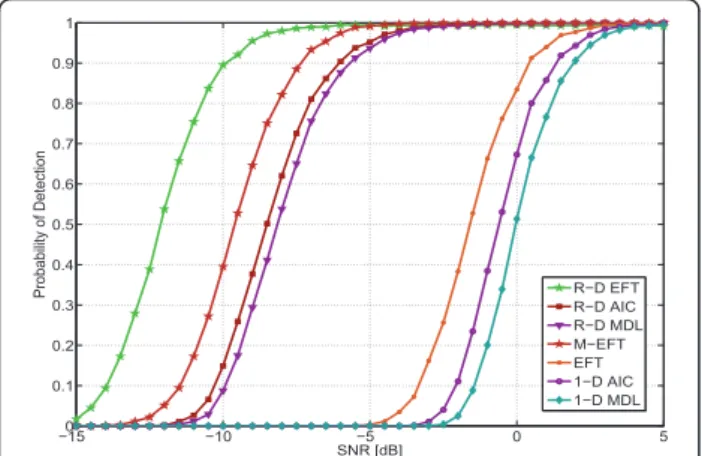
In Figures 7 and 8, we compare our proposed approach to all mentioned techniques for the case that white noise is present. To compare the performance of CFP-MOS for various values of the design parameter

Tlim, we selectTlim= 2 for the legend CFP 2f andTlim=

4 for CFP 4f. In Figure 7, the model orderdis equal to 2, while in Figure 8, d= 3. In these two scenarios, the

proposed CFP-MOS has a performance very close to R

-D EFT, which has the best performance.

In Figures 9 and 10, we assume the noise correlation structure of Equation (9), whereWiof theith factor for

Mi= 3 is given by

Wi=

⎡

⎣1 p

∗ i (p∗i)

2

pi 1 p∗_i

p2

i pi 1

⎤

⎦, (40)

whereri is the correlation coefficient. Note that also

other types of correlation models different from (40) can be used.

In Figures 9 and 10, the noise is colored with a very

high correlation, and the factors Li are computed

based on (9) and (40) as a function ofri. As expected

for this scenario, the R-D EFT, R-D AIC, and R-D

MDL completely fail. In case of colored noise with high correlation, the noise power is much more

−020 −15 −10 −5 0 5 10 15 20

0.1 0.2 0.3 0.4 0.5 0.6 0.7 0.8 0.9 1

SNR [dB]

Probability of Detection

T−CORCONDIA Var T−CORCONDIA Fix R−D EFT R−D AIC R−D MDL MOD EFT EFT AIC MDL

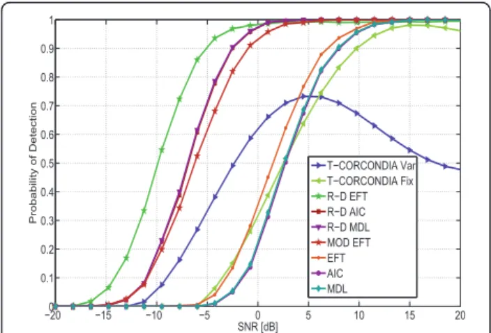
Figure 5Probability of correct Detection (PoD) versus SNR considering a system with a data model ofM1= 7,M2= 7,M3

= 7,M4= 7, andd= 3 sources.

−020 −15 −10 −5 0 5 10 15 20 25 30

0.1 0.2 0.3 0.4 0.5 0.6 0.7 0.8 0.9 1

SNR [dB]

T−CORCONDIA Var T−CORCONDIA Fix R−D EFT R−D AIC R−D MDL MOD EFT EFT AIC MDL

Figure 6Probability of correct Detection (PoD) versus SNR considering a system with a data model of M1= 7, M2= 7, M3

(10)

concentrated in the signal components. Therefore, the smaller are the values of d, the worse is the PoD. The behavior of the CFP-MOS, AIC, MDL, and EFT are consistent with this effect. The PoD of AIC, MDL, and EFT increases from 0.85, 0.7, and 0.7 in Figure 9 to 0.9, 0.85, and 0.85 in Figure 10. CFP-MOS 4f has a PoD = 0.98 for SNR = 20 dB in Figure 9, while a PoD = 0.98 for SNR = 15 dB in Figure 10.

In contrast to CFP-MOS, AIC, MDL, and EFT, the PoD of RADOI [22] degrades from Figures 9 and 10. In Figure 9, RADOI has a better performance than the CFP-MOS version, while in Figure 10, CFP-MOS out-performs RADOI. Note that the PoD for RADOI

becomes constant for SNR ≤3 dB, which corresponds

to a biased estimation. Therefore, for severely colored noise scenarios, the model order selection using CFP-MOS is more stable than the other approaches.

In Figure 11, no FBA is applied in all model order selection techniques, while in Figure 12 FBA is applied in all of them according to section 4. In general, an improvement of approximately 3 dB is obtained when FBA is applied.

In Figure 12, d = 3. Therefore, using the sequential definition of the global eigenvalues from“R-D Exponen-tial Fitting Test (R-D EFT)”, we can estimate the model order considering four modes. By increasing the number of sources to 5 in Figure 13, the sequential definition of the global eigenvalues is computed considering the sec-ond, third, and fourth modes, which are related toM2,

M3, andN.

By increasing the number of sources even more such that only one mode can be applied, the curves of the R

-D EFT, R-D AIC and R-D MDL are the same as the

curves of M-EFT, 1-D AIC, and 1-D MDL, as shown in Figure 14.

−15 −10 −5 0 5 10 0

0.1 0.2 0.3 0.4 0.5 0.6 0.7 0.8 0.9 1

SNR [dB]

R−D EFT R−D AIC RADOI M−EFT EFT AIC MDL CFP 2f CFP 4f

Figure 7Probability of correct Detection (PoD) versus SNR. In the simulated scenario,R= 5,M1= 5,M2= 5,M3= 5,M4= 5,M5=

5, andN= 5 presence of white noise. We fixedd= 2.

−020 −15 −10 −5 0 5 10 15 20 0.1

0.2 0.3 0.4 0.5 0.6 0.7 0.8 0.9 1

SNR [dB]

5, andN= 5 presence of white noise. We fixedd= 3.

0 5 10 15 20 25 30

0 0.1 0.2 0.3 0.4 0.5 0.6 0.7 0.8 0.9 1

SNR [dB]

5, andN= 5 presence of colored noise, where_r1= 0.9,r2= 0.95,

r3= 0.85, andr4= 0.8. We fixedd= 2.

0 2 4 6 8 10 12 14 16 18 20 0

0.1 0.2 0.3 0.4 0.5 0.6 0.7 0.8 0.9 1

SNR [dB]

5, andN= 5 presence of colored noise, wherer1= 0.9,r2= 0.95,

(11)

Conclusions

In this article, we have compared different model order selection techniques for multi-dimensional high-resolu-tion parameter estimahigh-resolu-tion schemes. We have achieved the following results considering a multi-dimensional data model.

1) In case of white Gaussian noise scenarios, our R-D EFT outperforms the other techniques presented in the literature.

2) In the presence of colored noise, the CFP-MOS is the best technique, since it has a performance close to the R-D EFT in case of no correlation, and a perfor-mance more stable than RADOI, in case of severely cor-related noise.

3) For researchers, which prefer to use information theoretic criteria (ITC) techniques, we have also pro-posed multi-dimensional extensions of AIC and MDL, calledR-D AIC andR-D MDL, respectively.

In Table 2, we summarize the scenarios to apply the different techniques shown in this article. Also in Table 2, wht stands for white noise and clr stands for colored noise. Note that the PoD of the CFP-MOS is close to

the one of the R-D EFT for white noise, which means

that it has a multi-dimensional gain. Moreover, since the CFP-MOS is suitable for white and colored noise applications, we consider it the best general-purpose scheme.

−015 −10 −5 0 5 0.1

0.2 0.3 0.4 0.5 0.6 0.7 0.8 0.9 1

SNR [dB]

Probability of Detection R−D EFT R−D AIC R−D MDL M−EFT EFT 1−D AIC 1−D MDL

Figure 11Probability of correct Detection (PoD) versus SNR for an array of sizeM1= 5,M2= 7, andM3= 9. The number of

snapshotsNis set to 10 and the number of sourcesd= 3. No FBA is applied.

−015 −10 −5 0 5 0.1

0.2 0.3 0.4 0.5 0.6 0.7 0.8 0.9 1

SNR [dB]

Probability of detection

R−D EFT FBA R−D AIC FBA R−D MDL FBA M−EFT FBA EFT FBA 1−D AIC FBA 1−D MDL FBA

snapshotsNis set to 10 and the number of sourcesd= 3. FBA is applied.

−015 −10 −5 0 5 0.1

0.2 0.3 0.4 0.5 0.6 0.7 0.8 0.9 1

SNR [dB]

snapshotsNis set to 10 and the number of sourcesd= 5. FBA is applied.

−015 −10 −5 0 5 0.1

0.2 0.3 0.4 0.5 0.6 0.7 0.8 0.9 1

SNR [dB]

(12)

Abbreviations

AIC: Akaike’s Information Criterion; CFP-MOS: closed-form PARAFAC-based model order selection; FBA: forward-backward averaging; HOSVD: higher-order SVD; MDL: minimum description length; MOS: model order selection; M-EFT: modified exponential fitting test; PoD: probability of correct detection;R-DEFT: R-dimensional Exponential Fitting Test; RESID: residuals; SMD: simultaneous matrix diagonalization; T-CORCONDIA: threshold core consistency analysis; ZMCSCG: zero-mean circularly symmetric complex Gaussian.

Acknowledgements

The authors gratefully acknowledge the partial support of the German Research Foundation (Deutsche Forschungsge-meinschaft, DFG) under contract no. HA 2239/2-1.

The authors would like to thank the anonymous reviewer for the comments, which improved the readability of this article.

Author details

1_{University of Brasília, Electrical Engineering Department, P.O. Box 4386,}

70910-900 Brasília, Brazil2Ilmenau University of Technology, Communications Research Laboratory P.O. Box 100565, 98684 Ilmenau, Germany

Competing interests

The authors declare that they have no competing interests.

Received: 22 December 2010 Accepted: 20 July 2011 Published: 20 July 2011

References

1. JPCL da Costa, M Haardt, F Roemer, G Del Galdo, Enhanced model order estimation using higher-order arrays, inProceedings of the 40th Asilomar

Conf. on Signals, Systems, and Computers,Pacific Grove, CA, USA

(November 2007)

2. JPCL da Costa, A Thakre, F Roemer, M Haardt, Comparison of model order selection techniques for high-resolution parameter estimation algorithms, in

Proceedings of the 54th International Scientific Colloquium(IWK_’09),Ilmenau,

Germany (October 2009)

3. JPCL da Costa,Parameter Estimation Techniques for Multi-dimensional Array

Signal Processing, 1st edn. (Shaker Publisher, Aachen, Germany,

March 2010)

4. JPCL da Costa, M Haardt, F Roemer, Robust methods based on HOSVD for estimating the model order in PARAFAC models, inProceedings of the IEEE

Sensor Array and Multichannel Signal Processing Workshop (SAM_’08),

Darmstadt, Germany (July 2008)

5. JPCL da Costa, F Roemer, M Weis, M Haardt, RobustR-D parameter estimation via closed-form PARAFAC, inProceedings of the ITG Workshop on

Smart Antennas (WSA_’10),Bremen, Germany (February 2010)

6. L De Lathauwer, B De Moor, J Vandewalle, A multilinear singular value decomposition.SIAMJ MatrixAnal Appl.21(4), 1253–1278 (2000). (26 pages)

7. F Roemer, M Haardt, A closed-form solution for parallel factor (PARAFAC) analysis, inProceedings of the IEEE International Conference on Acoustics, Speech

and Signal Processing (ICASSP 2008)Las Vegas, USA, pp. 2365–2368 (April 2008)

8. P Comon, JMF ten Berge, Generic and typical ranks of three-way arrays, in Proc. IEEE International Conference on Acoustics, Speech and Signal Processing

(ICASSP 2008),Las Vegas, USA, pp. 3313_–3316 (April 2008)

9. HM Huizenga, JC de Munck, LJ Waldorp, RPPP Grasman, Spatiotemporal EEG/MEG source analysis based on a parametric noise covariance model.

IEEE Trans Biomed Eng.49(6), 533–539 (2002). doi:10.1109/

TBME.2002.1001967

10. B Park, TF Wong, Training sequence optimization in MIMO systems with colored noise, inMilitary Communications Conference (MILCOM 2003), Gainesville, USA (October 2003)

11. JPCL da Costa, F Roemer, M Haardt, Sequential GSVD based prewhitening for multidimensional HOSVD based subspace estimation, inProceedings of

the ITG Workshop on Smart Antennas, Berlin, Germany(February 2009)

12. J Grouffaud, P Larzabal, H Clergeot, Some properties of ordered eigenvalues of a wishart matrix: application in detection test and model order selection,

inProceedings of the IEEE International Conference on Acoustics, Speech and

Signal Processing (ICASSP’96),5, 2463–2466 (May 1996)

13. A Quinlan, J-P Barbot, P Larzabal, M Haardt, Model order selection for short data: an exponential fitting test (EFT).EURASIP J Appl Signal Process.2007, 54–64 (2007)

14. F Roemer, M Haardt, A closed-form solution for multilinear PARAFAC decompositions, inProceedings of the 5th IEEE Sensor Array and Multichannel

Signal Processing Workshop (SAM 2008),Darmstadt, Germany, pp. 487_–491

(July 2008)

15. M Weis, F Roemer, M Haardt, D Jannek, P Husar, Multi-dimensional Space-Time-Frequency component analysis of event-related EEG data using closed-form PARAFAC, inProceedings of the IEEE International Conference Acoustics,

Speech, and Signal Processing (ICASSP 2009),Taipei, Taiwan (April 2009)

16. R Badeau, B David, G Richard, Selecting the modeling order for the ESPRIT high resolution method: an alternative approach, inProc. IEEE International Conference on Acoustics, Speech and Signal Processing (ICASSP 2004), Montreal, Canada (May 2004)

17. G Xu, RH Roy, T Kailath, Detection of number of sources via exploitation of centro-symmetry property.IEEE Trans Signal Process.42, 102_–112 (1994). doi:10.1109/78.258125

18. M Haardt, F Roemer, G Del Galdo, Higher-order SVD based subspace estimation to improve the parameter estimation accuracy in multi-dimensional harmonic retrieval problems.IEEE Trans Signal Process.56(7), 3198_–3213 (2008)

19. F Roemer, M Haardt, G Del Galdo, Higher order SVD based subspace estimation to improve multi-dimensional parameter estimation algorithms,

inProceedings of the 40th Asilomar Conference on Signals, Systems, and

Computers, pp. 961_–965 (November 2006)

20. A Lee, Centrohermitian and skew-centrohermitian matrices.Linear Algebra Appl.29, 205–210 (1980). doi:10.1016/0024-3795(80)90241-4

Table 2 Summarized table comparing characteristics of the multi-dimensional model order selection schemes

Scheme Minimumd Maximumd Noise Performance

T-CORCONDIA [21,4] 1 Typical rank [8] Wht and clr Comparable to 1-D AIC

R-D AIC [4,1] 0 max

r (

min

Mr,

M

Mr

−1

)

Wht Superior to 1-D AIC

R-D MDL [4,1] 0 max

r (

min

Mr,

M

Mr

−1

)

Wht Superior to 1-D MDL

R-D EFT [4,1] 0 max

r (

min

Mr,

M

Mr

−1

)

Wht Best

CFP-MOS [5] 1 max

(13)

21. R Bro, HAL Kiers, A new efficient method for determining the number of components in PARAFAC models. J Chemom.17, 274_–286 (2003). doi:10.1002/cem.801

22. E Radoi, A Quinquis, A new method for estimating the number of harmonic components in noise with application in high resolution radar.

EURASIP J Appl Signal Process.2004(8), 1177_–1188 (2004). doi:10.1155/

S1110865704401097

doi:10.1186/1687-6180-2011-26

Cite this article as:da Costaet al.:Multi-dimensional model order

selection.EURASIP Journal on Advances in Signal Processing20112011:26.