A comparison of stochastic systems with different types of delays

(1)

A Comparison Of Stochastic Systems With

Different Types Of Delays

H.T. Banks, Jared Catenacci and Shuhua Hu

Center for Research in Scientific Computation

,

North Carolina State University

Raleigh, NC 27695-8212

March 26, 2013

Abstract

In this paper we investigate the effects of different types of delays, a fixed delay and a random delay, on the dynamics of stochastic systems as well as their relationship with each other in the context of a just-in-time network model. The specific example on which we focus is a pork production network model. We numerically explore the corresponding deterministic approximations for the stochastic systems with these two different types of delays. Numerical results reveal that the agreement of stochastic systems with fixed and random delays depend upon the population size and the variance of the random delay, even when the mean value of the random delay is chosen the same as the value of the fixed delay. When the variance of the random delay is sufficiently small, the histograms of state solutions to the stochastic system with a random delay are similar to those of the stochastic model with a fixed delay regardless of the population size. We also compared the stochastic system with a Gamma distributed random delay to the stochastic system constructed based on the Kurtz’s limit theorem from a system of deterministic delay differential equations with a Gamma distributed delay. We found that with the same population size the histogram plots for the solution to the second system appear more dispersed than the corresponding ones obtained for the first case. In addition, we found that there is more agreement between the histograms of these two stochastic systems as the variance of the Gamma distributed random delay decreases.

Key Words: systems with delays, Markov Chain stochastic vs. deterministic approximations, Kurtz

limit theorem, fixed vs. random delays, Gamma distribution and the linear chain trick.

1

Introduction

Continuous time Markov Chain models are widely used to model physical and biological processes (e.g., see [1, 3]). These models are typically (and most appropriately) used when dealing with dynamic systems involving low species count. In stochastic modeling one often wishes to know whether or not the stochastic system can be approximated by a deterministic one when the population size is sufficiently large. Theory established by Kurtz (e.g., [14, 15, 16]), provides a way to construct a deterministic system to approximate density dependent continuous time Markov Chains as the population size grows large (this result is often called the Kurtz’s limit theorem, see details below). In general, deterministic systems are much easier to analyze compared to stochastic systems. Techniques, such as parameter estimation methods, are well developed for deterministic systems, whereas parameter estimation is much more difficult in a stochastic framework (e.g., see [22]).

(2)

referred to stochastic models with delays in this paper) have enjoyed considerable research attention in the past decade, especially the efforts on the development of algorithms to simulate such systems (e.g., [2, 7, 10, 24]). However, to the best of our knowledge, it appears that there is a dearth of efforts on the convergence of solutions to stochastic system with delays as the sample size goes to infinity (that is, an analogy of Kurtz’s limit theorem). The two works that we found are the results presented in [9] and [26]. Specifically, Bortolussi and Hillston [9] extended the Kurtz’s limit theorem to the case where fixed delays are incorporated into a density dependent continuous time Markov chain. Schlicht and Winkler [26] showed that if all the transition rates are linear, then the mean solution of stochastic system with random delays can be described by deterministic differential equations with distributed delays. However, to our knowledge, there are still no theoretical results on the convergence of solutions to a general stochastic system with random delays. That is, there is still no analog of the Kurtz’s limit theorem for a general stochastic system with random delays.

As a first step, in this paper we numerically explore the corresponding deterministic differential equations for the stochastic systems with delays, and investigate the effects of different types of delays on the dynamics of stochastic systems as well as their relationship with each other. Specifically, we do this in the context of an extension of the pork production network model in [4] to incorporate delays which account for the phenomenon that the movement from one node to the next is often not instantaneous nor deterministic. Before addressing our main tasks, we shall use this introduction to give a brief review of Kurtz’s limit theorem in Section 1.1 and the original pork production model in Section 1.2.

1.1

The Kurtz’s limit theorem

Let ν be a positive integer number, and Zν be the set of ν-dimensional column vectos with integer com-ponents. Suppose for each positive number N, {XN(t), t ≥0} with state space XN _⊂

Zν is a continuous time Markov chain with transition rateλj(xN) at the jth transition (often referred to asreactions in the

biochemistry literature),j= 1,2,3, . . . , M withM being the number of transitions. In other words, for any small time interval ∆twe have

Prob©

XN(t+ ∆t) =xN +vj|XN(t) =xNª=λj(xN)∆t+o(∆t), j= 1,2, . . . , M, (1)

where vj = (v1j, v2j, v3j, . . . , vνj)T ∈Zν with vij denoting the change in state variableXiN caused by the

jth transition. This family of continuous time Markov chain is calleddensity dependentif and only if there exist continuous functionsfj:Rν →Rsuch that

λj(x) =N fj(x/N), j= 1,2, . . . , M. (2)

This process can be characterized by standard Poisson processes (e.g., see [3, 12]), that is, XN(t) can be written as

XN(t) =XN(0) +

M

X

j=1

vjYj

µZ t

0

λj(XN(s))ds

¶

, (3)

where {Yj(t), t ≥0}, j = 1,2, . . . , M are independent standard Poisson processes. LetCN(t) =XN(t)/N.

Then we obtain another continuous time Markov chain{CN(t), t≥0}. Define

g(c) =

M

X

j=1

vjfj(c).

Then by (2) and (3), one can use the strong law of large numbers to show that with some mild conditions on

gandfj the processes{CN(t), t≥0}converges to a deterministic process that is the solution of the system

of ordinary differential equations

˙

c(t) =g(c), c(0) =c0. (4)

(3)

Theorem 1. Suppose that lim

N→∞C

N_{(0) =}_c

0and for any compact setΩ⊂Rν there exists a positive constant ηΩ such that

|g(c)−g(˜c)| ≤ηΩ|c−˜c|, c,˜c∈Ω. (5)

Then we have

lim

N→∞tsup≤tf

|CN(t)−c(t)|= 0 a.s. for alltf >0, (6)

wherec(t)denotes the unique solution to (4).

Theorem 1 indicates that the convergence is in the sense of convergence almost surely. It is worth noting that in Kurtz’s original work [14, 15] the convergence is in the sense of convergence in probability. In addition, it should be noted that based on the problem considered, the parameterN can be interpreted as the total number in a population, the volume of the population occupied, or some other scaling factor. Hence, the parameterN is often called the population size, the sample size, or scaling parameter. For notational convenience, we suppress the dependence onN in much of the remainder of this paper (i.e., if no confusion occurs). Thus, we simply denoteXN byXandCN byC.

1.2

The original pork production network model

In current production methods for livestock based on a just-in-time philosophy, animals are grown in different areas, and are moved from one farm to another depending on their age. Unfortunately, shocks propagate rapidly through such systems, and may cause devastating effects on their performance. For example, stop-ping movement of animals to and from a farm with animals infected by a disease will have effects that quickly spread through the whole system: nurseries supplying the farm will have nowhere to send their animals as they grow up, and finishers and slaughterhouses supplied by the farm will have their supply interrupted. Hence, it is of great interest to identify bottlenecks in the production and feed supply chain, and to test potential mitigation tools, procedures, and practices to increase the resilience of animal agriculture to catas-trophic events. Motivated by this, a stochastic pork production network model was developed in [4] to investigate how small perturbations to the agricultural supply system would affect its overall performance.

We give a brief review of the the pork production model developed in [4]; interested readers can refer to [4] for more information. In this model, four nodes of production are considered: sows, nurseries, fin-ishers, and slaughterhouses. The movement of pigs from one node to the next is assumed to occur only in the forward direction. That is, from sows to nurseries, from nurseries to finishers and from finishers to slaughterhouses. The population (N) is assumed to remain constant, and thus, the number of deaths that occur at the slaughterhouses is taken to be the same as number of births at the sows node. The evo-lution of the system is modeled using a continuous time Markov Chain with states at time t denoted by

X(t) = (X1(t), X2(t), X3(t), X4(t))T, where Xi(t) is the number of pigs at theith node at timet.

Furthermore, the model assumes that there is a capacity constraint (Li) at each node with a maximal

exit constraintSmat node 4. Letei∈Z4 be theith unit column vector, that is, theith entry ofei is 1 and

all the other entries are zeros, i = 1,2,3,4. The transition rate λj(x) and the corresponding state change

vectorvj at thejth transition, j= 1,2,3,4, are given by

λ1(x) =k1x1(L2−x2)+, v1=−e1+e2,

λ2(x) =k2x2(L3−x3)+, v2=−e2+e3,

λ3(x) =k3x3(L4−x4)+, v3=−e3+e4,

λ4(x) =k4min(x4, Sm), v4=−e4+e1,

where (z)+ = max(z,0), and ki is the service rate at node i, i = 1,2,3,4. Then by (3) we know that the

pork production network can be described by the following stochastic system.

X1(t) =X1(0)−Y1

µZ t

0

λ1(X(s))ds

¶

+Y4 µZ t

0

λ4(X(s))ds

¶

X2(t) =X2(0)−Y2

µZ t

0

λ2(X(s))ds

¶

+Y1 µZ t

0

λ1(X(s))ds

¶

X3(t) =X3(0)−Y3

µZ t 0

λ3(X(s))ds

¶

+Y2 µZ t

0

λ2(X(s))ds

¶

X4(t) =X4(0)−Y4

µZ t

0

λ4(X(s))ds

¶

+Y3 µZ t

0

λ3(X(s))ds

¶ .

(4)

There are a number of algorithms that can be used to simulate a stochastic system such as (7) (e.g., see [23] for a recent review of such algorithms). Here we will outline one of them, the modified next reaction method (NRM) algorithm, which is a modification to the next reaction method of Gibson and Bruck [11]. The NRM algorithm was developed by Anderson in [2], wherein the next reaction method of Gibson and

Bruck was modified to make more explicit use of the “internal times”, which are defined as

Z t 0

λi(X(s))ds

for each transition. One of the advantages of the modified next reaction algorithm is that it can be easily extended to simulate stochastic systems with time dependent transition rates whereas the next reaction method can not. In addition, the NRM algorithm can be altered to simulate stochastic systems with fixed delays, and further altered to simulate stochastic systems with random delays.

Suppose the stochastic system to be simulated has M ≥ 1 transitions with transition rates λi(x) for

i= 1,2, . . . , M. Then the NRM algorithm is given as follows.

Algorithm 1: Modified Next Reaction Method

1. Set the initial condition for each state att= 0. SetTi= 0 fori= 1,2, . . . , M.

2. Calculate each transition rateλi at the given state fori= 1,2, . . . , M.

3. GenerateM independent, uniform (0,1) random numbers ri.

4. SetPi= ln(1/ri) fori= 1,2, . . . , M.

5. Set ∆ti= (Pi−Ti)/λi fori= 1,2, . . . , M.

6. Set ∆ = min

1≤i≤M(∆ti), and letl be the reaction which obtains the minimum.

7. Sett=t+ ∆.

8. Update the system based on the reactionl. 9. SetTi=Ti+λi∆ for i= 1,2, . . . , M.

10. For transitionl, choose a uniform random number (0,1),r, and setPl=Pl+ ln(1/r).

11. Recalculate each transition rateλi at the given new state fori= 1,2, . . . , M.

12. Return to step 5.

As in [4], if we rescale the stochastic system (7) in such a way that instead of following the number of pigs at each node we track the concentration of pigs (i.e.,C(t) =X(t)/N where N = Σ4i=1Xi(t)), then by

Kurtz’s limit theorem we know that the appropriate rescaling allows us to obtain an approximating system of ordinary differential equations (ODE’s) for the scaled stochastic system C(t). Rescale the constants as follows:

κ4=k4, κi=N ki, i= 1,2,3

sm=SM/N, li=Li/N.

Then the resulting approximating system of ODE’s is given by

˙

c1(t) =−κ1c1(t)(l2−c2(t))++κ4min(c4(t), sm)

˙

c2(t) =−κ2c2(t)(l3−c3(t))++κ1c1(t)(l2−c2(t))+

˙

c3(t) =−κ3c3(t)(l4−c4(t))++κ2c2(t)(l3−c3(t))+

˙

c4(t) =−κ4min(c4(t), sm) +κ3c3(t)(l4−c4(t))+

c(0) =c0,

(8)

wherec(t) = (c1(t), c2(t), c3(t), c4(t))T, andc0= (c10, c20, c30, c40)T.

2

The Pork Production Network Model With A Fixed Delay

(5)

long distance between the nodes, bad weather or some other disruptions/interruptions. Presented here is a first attempt to account for delays in the following way. Assume that all transitions occur instantaneously except for the arrival of pigs transitioning from node 1 to 2. That is, the pigs leave node 1 immediately, but the time of arrival at node 2 is delayed. For simplicity, we only consider a delay in one of the transitions, but depending on the physical proximity of the nodes, it may be a reasonable assumption to have delays in even more of the transitions.

2.1

The stochastic model with a fixed delay

As a first and simplest consideration, we take the delayed time of arrival at node 2,τ, to be a fixed value. If we assume that the process starts fromt= 0 (that is,X(t) = 0 for t <0), then this results in a stochastic model with a fixed delay given by

X1(t) =X1(0)−Y1

µZ t

0

λ1(X(s))ds

¶

+Y4 µZ t

0

λ4(X(s))ds

¶

X2(t) =X2(0)−Y2

µZ t 0

λ2(X(s))ds

¶

+Y1 µZ t

0

λ1(X(s−τ))ds

¶

X3(t) =X3(0)−Y3

µZ t

0

λ3(X(s))ds

¶

+Y2 µZ t

0

λ2(X(s))ds

¶

X4(t) =X4(0)−Y4

µZ t

0

λ4(X(s))ds

¶

+Y3 µZ t

0

λ3(X(s))ds

¶ .

(9)

Note thatλ1 only depends on the state. Hence, the assumption ofX(t) = 0 fort <0 leads to λ1(X(t)) = 0

fort <0. The interpretation of this stochastic model with a fixed delay (9) is as follows. When any of the

transitionsλ2,λ3or λ4 fires at timet, the system is updated accordingly at timet. When the transitionλ1

fires at timet, one unit is subtracted from the first node. Since the completion of the transition is delayed, at timet+τ the unit is added onto node 2.

2.2

Algorithms for stochastic systems with fixed delays

In this section we outline one possible algorithm that may be used to simulate a stochastic system such as (9) with fixed delays. This modified next reaction method for systems with delays algorithm is given in [2]. In general, there are three types of reactions to consider. First are the reactions with no delay (ND). Second are the reactions where they only affect the state of the system upon completion (CD). And finally, the reactions where the state of the system is affected at the initiation and the completion of the reaction (ICD). In the example case here the delayed reaction is an ICD. As before letM ≥1 be the number of transitions with transition ratesλi(x) fori= 1,2, . . . , M. In addition, if thejth transition is a delayed one, then we let

τj denote the delay time between the initiation and completion for this transition.

Algorithm 2: Modified Next Reaction Method For Stochastic Systems With Fixed Delays

1. Set the initial condition for each state att= 0. SetTi= 0, and the arraymi = (∞) fori= 1,2, . . . , M.

2. Calculate each transition rateλi at the given state fori= 1,2, . . . , M.

4. SetPi= ln(1/ri) fori= 1,2. . . , M.

6. Set ∆ = min

1≤i≤M(∆ti,mi(1)−t).

7. Sett=t+ ∆.

8. If ∆tl obtained the minimum in step 6 then do the following. If thel reaction is a ND, then update

the system according to the reactionl. If reactionlis a CD then store the timet+τlin the second to

last position in ml. If reaction l is a ICD then update the system according to the initiation of thel

reaction and storet+τlin the second to last position in ml.

9. If ml(1)−t obtained the minimum in step 6 then update the system according the completion of

(6)

10. SetTi=Ti+λi∆ for i= 1,2, . . . , M.

11. For transitionl which initiated, choose a uniform random number (0,1),r, and setPl=Pl+ ln(1/r).

13. Return to step 5.

2.3

The corresponding deterministic system for the stochastic model with a

fixed delay

In [9], Bortolussi and Hillston extended the Kurtz’s limit theorem to a scenario with fixed delays incorporated into a density dependent continuous time Markov chain, where the convergence is in the sense of convergence in probability. We will use our pork production model (9) to illustrate this theorem (referred to as the BH limit theorem). Using the same rescaling procedure as before (C(t) =X(t)/N withX(t) described by (9)), an approximating deterministic system can be constructed based on the BH limit theorem for the scaled stochastic system with a fixed delay. This approximating deterministic system is given by

˙

c2(t) =−κ2c2(t)(l3−c3(t))++κ1c1(t−τ)(l2−c2(t−τ))+

˙

c3(t) =−κ3c3(t)(l4−c4(t))++κ2c2(t)(l3−c3(t))+

˙

c4(t) =−κ4min(c4(t), sm) +κ3c3(t)(l4−c4(t))+.

(10)

We note that this approximating deterministic system is no longer a system of ordinary differential equations, but rather a system of delay (ordinary) differential equations with a fixed delay. The delay differential equation is a direct result of the delay term present in (9). Since there is a delay term, the system is dependent on the previous states, for this reason it is necessary to have some past history functions as initial conditions. It should be noted that past history functions should notbe chosen in an arbitrary fashion as they should capture the limit dynamics of the scaled stochastic system with a fixed delay.

Next we illustrate how to construct the initial conditions for the delay differential equation (10). We observe that in the interval [0, τ] the delay term has no affect, thus we can ignore the delay term in this interval. This yields a stochastic system with no delays, the concentration of which can be approximated by a system of ODE’s as was done previously. This gives the deterministic system

˙

c2(t) =−κ2c2(t)(l3−c3(t))+

˙

c3(t) =−κ3c3(t)(l4−c4(t))++κ2c2(t)(l3−c3(t))+

˙

c(0) =c0

(11)

for t ∈ [0, τ]. We let Φ(t) denote the solution to (11) and thus we have that C(t) converges to Φ(t) as

N → ∞on the interval [0, τ].

In the interval [τ, tf], where tf is the final time, the delay has an affect, so we approximate with the

DDE system (10), and the solutionΦ(t) to the ODE (11) on the interval [0, τ] serves as the initial function. Explicitly the system can be written as

˙

c2(t) =−κ2c2(t)(l3−c3(t))++κ1c1(t−τ)(l2−c2(t−τ))+

˙

c3(t) =−κ3c3(t)(l4−c4(t))++κ2c2(t)(l3−c3(t))+

˙

c(s) =Φ(s), s∈[0, τ]. (12)

The BH limit theorem indicates thatC(t) converges in probability to the solution of (12) asN → ∞.

Remark 2. We remark that in the literature one often sees an arbitrarily chosen past history function for

(7)

2.4

Comparison of the stochastic model with a fixed delay and its corresponding

deterministic system

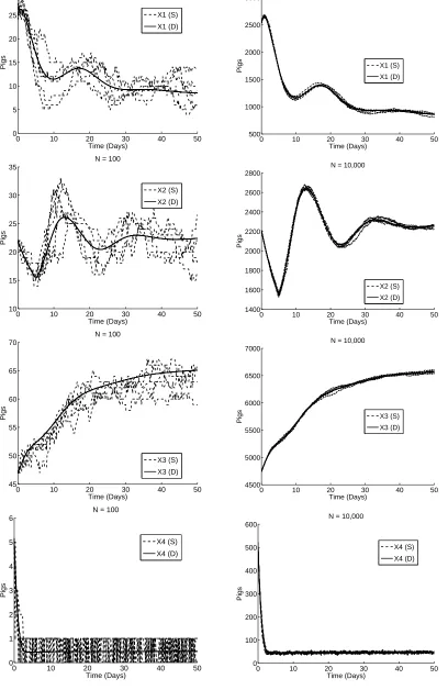
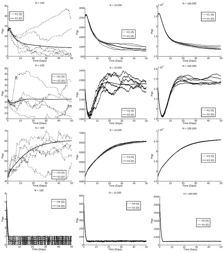
In this section we compare the results of the stochastic system with a fixed delay (9) to its corresponding deterministic system (in terms of number of pigs, i.e., Nc(t) with c(t) being the solution to (12)). The stochastic system with a fixed delay (9) was simulated using Algorithm 2 in Section 2.2, and the deterministic system (12) was solved numerically using a linear spline approximation method (e.g., see [5, 6] for details).

All parameter values and initial conditions are taken from [4] and are given in Table 1. The value of

Parameters Values Units Parameters Values Units

k1 1.674/N 1/(pigs·days) κ1 1.674 1/days

k4 1 1/days κ4 1 1/days

L1 ∞ pigs

L2 N·2.607·10−1 pigs l2 2.607·10−1 dimensionless L3 N·7.267·10−1 pigs l3 7.267·10−1 dimensionless L4 N·6.3·10−3 pigs l4 6.3·10−3 dimensionless Sm N·1.39·10−1 pigs sm 1.39·10−1 dimensionless

X1(0) [N·2.528·10−1] pigs c1(0) 2.528·10−1 dimensionless X2(0) [N·2.212·10−1] pigs c2(0) 2.212·10−1 dimensionless X3(0) [N·4.739·10−1] pigs c3(0) 4.739·10−1 dimensionless X4(0) [N·5.21·10−2] pigs c4(0) 5.21·10−2 dimensionless

Table 1: Parameter values and initial conditions for the stochastic and deterministic systems, where N is the scaling parameter and[z]denotes the integer closest to z.

(8)

0 10 20 30 40 50 0

5 10 15 20 25 30

N = 100

Time (Days)

Pigs

X1 (S)

X1 (D)

0 10 20 30 40 50

500 1000 1500 2000 2500 3000

N = 10,000

Time (Days)

Pigs X1 (S)

X1 (D)

0 10 20 30 40 50

10 15 20 25 30 35

N = 100

Time (Days)

Pigs

X2 (S)

X2 (D)

0 10 20 30 40 50

1400 1600 1800 2000 2200 2400 2600 2800

N = 10,000

Time (Days)

Pigs

X2 (S)

X2 (D)

0 10 20 30 40 50

45 50 55 60 65 70

N = 100

Time (Days)

Pigs

X3 (S)

X3 (D)

0 10 20 30 40 50

4500 5000 5500 6000 6500 7000

N = 10,000

Time (Days)

Pigs X3 (S)

X3 (D)

0 10 20 30 40 50

0 1 2 3 4 5 6

N = 100

Time (Days)

Pigs

X4 (S) X4 (D)

0 10 20 30 40 50

0 100 200 300 400 500 600

N = 10,000

Time (Days)

Pigs

X4 (S)

X4 (D)

(9)

deter-0 10 20 30 40 50 5

10 15 20 25 30

N = 100

Time (Days)

Pigs

X1 (S)

X1 (D)

0 10 20 30 40 50

500 1000 1500 2000 2500 3000

N = 10,000

Time (Days)

Pigs X1 (S)

X1 (D)

0 10 20 30 40 50

14 16 18 20 22 24 26 28

N = 100

Time (Days)

Pigs

X2 (S)

X2 (D)

0 10 20 30 40 50

1400 1600 1800 2000 2200 2400 2600 2800

N = 10,000

Time (Days)

Pigs

X2 (S)

X2 (D)

0 10 20 30 40 50

45 50 55 60 65 70

N = 100

Time (Days)

Pigs X3 (S)

X3 (D)

0 10 20 30 40 50

4500 5000 5500 6000 6500 7000

N = 10,000

Time (Days)

Pigs X3 (S)

X3 (D)

0 10 20 30 40 50

0 1 2 3 4 5 6

N = 100

Time (Days)

Pigs

X4 (S) X4 (D)

0 10 20 30 40 50

0 100 200 300 400 500 600

N = 10,000

Time (Days)

Pigs

X4 (S)

X4 (D)

(10)

3

The Pork Production Network Model With A Random Delay

We next address the issue of how to implement random delays into the original pork production model. In the previous section we assumed that the delay was fixed. The interpretation of that formulation is that every transition from node 1 to node 2 is delayed by the same amount of time. We now want to consider the case where the amount of delayed time varies at each transition. The motivation for doing so is that in practice we would expect that the amount of time it takes to travel from node 1 to node 2 will vary based on a number of conditions, e.g., weather, traffic, road construction, etc. In this case it may not be a reasonable assumption that every transition is delayed by the same amount of time, but rather may vary for each transition that occurs. One way to implement this variation of delay times is to consider the delay to be a random variable that will be sampled for each transition. The resulting system will be called the stochastic model with a random delay. For this model, we again assume that all transitions occur instantaneously except for the arrival of pigs transitioning from node 1 to 2, and the process starts from t = 0, that is,

X(t) = 0 fort <0.

3.1

Algorithms for stochastic systems with random delays

Roussel and Zhu propose a method in [24] for simulating a stochastic system with random delays. Specifically, the algorithm for a stochastic system with random delays can be implemented in a way that is a slight modification of Algorithm 2 in Section 2.2. The algorithm simulates which reaction will take place next. In the case of fixed delays, if a delayed transition fires, then the effect of that transition is held until the specified amount of time passes. In the case of random delays, when a delayed transition occurs, the delay is sampled from a given distribution, and this value is taken as the amount of time that must pass before the transition affects the system. Each time a delayed transition is fired, a new value of the delay is drawn from the given distribution. The full details of the algorithm are outlined below.

When a delayed reaction fires, one draws a random number from the desired distribution to use for the delay. Previously, in the fixed delay case, all that was needed was to store the delayed time in the arraymlin

the second to last position. This guaranteed that the arraymlwas sorted in ascending order (recall that the

last element inml was initialized to infinity). If the delay is random we cannot take this approach, instead

the delayed time must be stored inml(in any position) and thenmlmust be sorted in ascending order. Let

us again assume that the stochastic system hasM transitions with transition ratesλi(x) fori= 1,2, . . . , M.

In addition, if thejth transition is a delayed one, then we letτjdenote the delay time between the initiation

and completion for this transition, where its value is sampled from a given distribution at each time this delayed transition is fired.

Algorithm 3: Modified Next Reaction Method For Stochastic Systems With Random Delays

1. Set the initial condition for each state for t= 0. SetTi= 0, and arraymi= (∞) fori= 1,2, . . . , M.

2. Calculate each transition rateλi at the given state for eachi= 1,2, . . . , M.

4. SetPi= ln(1/ri) fori= 1,2, . . . , M.

6. Set ∆ = min1≤i≤M(∆ti,mi(1)−t).

7. Sett=t+ ∆.

8. If ∆tlobtained the minimum in step 6 then do the following. If thelreaction is a ND, then update the

system according to the reactionl. If reactionlis a CD then store the timet+τlinmland sortml in

ascending order, whereτl is sampled from a given distribution. If reactionl is a ICD then update the

system according to the initiation of thelreaction and storet+τlinmland then sortmlin ascending

order, where τl is sampled from a given distribution.

9. If ml(1)−t obtained the minimum in step 6 then update the system according the completion of

reaction land delete the first element in ml.

10. SetTi=Ti+λi∆ for i= 1, . . . , M.

11. For the transitionlwhich initiated, choose a uniform random number (0,1),r, and setPl=Pl+ln(1/r).

(11)

3.2

The corresponding deterministic system for the stochastic model with a

random delay

In [26], Schlicht and Winkler showed that if all the transition rates arelinear, then the mean solution of the stochastic system with random delays can be described by a system of deterministic differential equations with a distributed delay, where the delay kernel is the probability density function of the given distribution for the random delay. Even though the transition rates in our pork production model arenonlinear, we still would like to explore whether or not such a deterministic system can be used as a possible corresponding deterministic system for our stochastic system with a random delay and explore the relationship between them.

LetG(t) be the probability density function of the random delay. Then the corresponding deterministic system for our stochastic system with delay is given by

˙

c2(t) =−κ2c2(t)(l3−c3(t))++

Z t

−∞

G(t−s)κ1c1(s)(l2−c2(s))+ds

˙

c3(t) =−κ3c3(t)(l4−c4(t))++κ2c2(t)(l3−c3(t))+

˙

ci(0) =ci0, i= 1,2,3,4,

ci(s) = 0, s <0, i= 1,2,3,4,

(13)

We note that numerically solving a system of the form (13) may prove to be difficult due to the distributed delay term. However, if we make additional assumptions on the delay kernel, we can transform a system with a distributed delay into a system of ODE’s. Specifically, if we assume that the delay kernel has the form

G(u;α, n) = α

n_un−1_e−αu

(n−1)! (14)

withα >0 andnbeing a positive integer number, that is,Gis the probability density function of a Gamma

distributed random variable with mean being n/αand the variance being n/α2_{, then by way of the linear}

chain trick [13] (e.g., see [8, 18, 25] and the references therein) we can transform the system (13) into a

system of ODE’s. For example, for the case n= 1, if we let c5(t) = Z t

−∞

αe−α(t−θ)κ1c1(θ)(l2−c2(θ))+dθ,

then this substitution yields the system of ODE’s

˙

c2(t) =−κ2c2(t)(l3−c3(t))++c5(t)

˙

c3(t) =−κ3c3(t)(l4−c4(t))++κ2c2(t)(l3−c3(t))+

˙

c5(t) =ακ1c1(t)(l2−c2(t))+−αc5(t)

ci(0) =ci0, i= 1,2,3,4,

c5(0) =

Z 0

−∞

αeαθ_κ

1c1(θ)(l2−c2(θ))+dθ.

(15)

which is equivalent to (13).

The advantage of using this linear chain trick is two fold. The resulting system of ODE’s is much easier to solve compared to the system (13) where there is a distributed delay. In addition, we can use the Kurtz’s limit theorem to construct a corresponding stochastic system which converges to the resulting system of ODE’s. This approach will be considered in Section 3.4.

3.3

Comparison of the stochastic model with a random delay and its

corre-sponding deterministic system

(12)

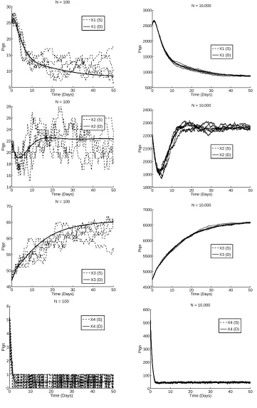
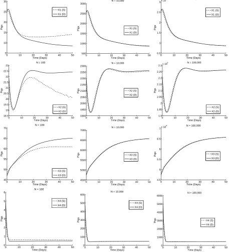
Figure 3 compares the solution of deterministic system (in terms of number of pigs, i.e., Nc(t) with

c(t) being the solution to (15)) and five typical sample paths of the solution to the stochastic system with a random delay. We observe from this figure that the trajectories of the stochastic simulations follow the

0 10 20 30 40 50

5 10 15 20 25 30

N = 100

Time (Days)

Pigs

X1 (S)

X1 (D)

0 10 20 30 40 50

500 1000 1500 2000 2500 3000

N = 10,000

Time (Days)

Pigs X1 (S)

X1 (D)

0 10 20 30 40 50

14 16 18 20 22 24 26 28

N = 100

Time (Days)

Pigs

X2 (S)

X2 (D)

0 10 20 30 40 50

1800 1900 2000 2100 2200 2300 2400

N = 10,000

Time (Days)

Pigs X2 (S)

X2 (D)

0 10 20 30 40 50

45 50 55 60 65 70

N = 100

Time (Days)

Pigs

X3 (S)

X3 (D)

0 10 20 30 40 50

4500 5000 5500 6000 6500 7000

N = 10,000

Time (Days)

Pigs X3 (S)

X3 (D)

0 10 20 30 40 50

0 1 2 3 4 5 6

N = 100

Time (Days)

Pigs

X4 (S)

X4 (D)

0 10 20 30 40 50

0 100 200 300 400 500 600

N = 10,000

Time (Days)

Pigs

X4 (S)

X4 (D)

(13)

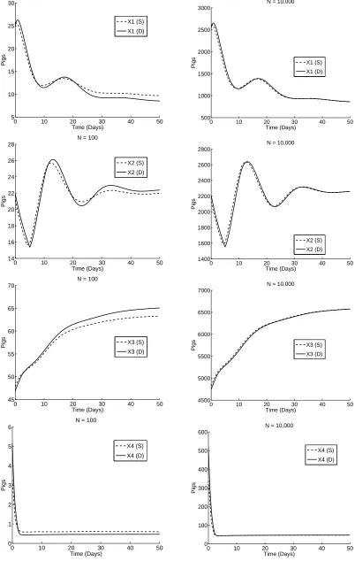
solution of the deterministic system, and the variation of the sample paths of the solution to the stochastic system with a random delay decreases as the sample size increases. Figure 4 depicts the mean solution for the stochastic system with a random delay in comparison to the solution of deterministic system (in terms of number of pigs). It is seen from this figure that as the sample size increases the mean solution of the stochastic

0 10 20 30 40 50

5 10 15 20 25 30

N = 100

Time (Days)

Pigs

X1 (S)

X1 (D)

0 10 20 30 40 50

500 1000 1500 2000 2500 3000

N = 10,000

Time (Days)

Pigs X1 (S)

X1 (D)

0 10 20 30 40 50

19 19.5 20 20.5 21 21.5 22 22.5 23

N = 100

Time (Days)

Pigs

X2 (S)

X2 (D)

0 10 20 30 40 50

1900 1950 2000 2050 2100 2150 2200 2250 2300

N = 10,000

Time (Days)

Pigs X2 (S)

X2 (D)

0 10 20 30 40 50

45 50 55 60 65 70

N = 100

Time (Days)

Pigs X3 (S)

X3 (D)

0 10 20 30 40 50

4500 5000 5500 6000 6500 7000

N = 10,000

Time (Days)

Pigs X3 (S)

X3 (D)

0 10 20 30 40 50

0 1 2 3 4 5 6

N = 100

Time (Days)

Pigs

X4 (S)

X4 (D)

0 10 20 30 40 50

0 100 200 300 400 500 600

N = 10,000

Time (Days)

Pigs

X4 (S)

X4 (D)

(14)

system with a random delay become closer to the solution of deterministic system. Hence, not only are the sample paths of the solution to stochastic system with a random delay showing less variation for larger sample sizes, but the expected value of the solution is better approximated by the solution of deterministic system for large sample sizes. Thus, the deterministic system (15) (or the deterministic differential equation with a distributed delay (13)) could be used to serve as a reasonable corresponding deterministic system for this particular stochastic system with a random delay (with the given parameter values and initial conditions).

3.4

The corresponding constructed stochastic system for the system of ODE’s

(15)

Based on the Kurtz’s limit theorem, one can construct a stochastic system (without delays) which will converge to the system of ODE’s given in (15). Let ei ∈Z5 be theith unit column vector, i= 1,2, . . . ,5.

The transition rateλj(x) and the corresponding state change vectorvj at thejth transition,j= 1,2, . . . ,7,

are given by

λ1(x) =k1x1(L2−x2)+, v1=−e1,

λ2(x) =k2x2(L3−x3)+, v2=−e2+e3,

λ3(x) =k3x3(L4−x4)+, v3=−e3+e4,

λ4(x) =k4min(x4, Sm), v4=−e4+e1

λ5(x) =x5, v5=e2

λ6(x) =αx5, v6=−e5

λ7(x) =αk1x1(L2−x2)+, v7=e5.

Then by (3) we know that the stochastic system corresponding to the above transitions rates and state change vectors is given by

X1(t) =X1(0)−Y1

µZ t 0

λ1(X(s))ds

¶

+Y4 µZ t

0

λ4(X(s))ds

¶

X2(t) =X2(0)−Y2

µZ t 0

λ2(X(s))ds

¶

+Y5 µZ t

0

λ5(X(s))ds

¶

X3(t) =X3(0)−Y3

µZ t

0

λ3(X(s))ds

¶

+Y2 µZ t

0

λ2(X(s))ds

¶

X4(t) =X4(0)−Y4

µZ t

0

λ4(X(s))ds

¶

+Y3 µZ t

0

λ3(X(s))ds

¶

X5(t) =X5(0)−Y6

µZ t 0

λ6(X(s))ds

¶

+Y7 µZ t

0

λ7(X(s))ds

¶ .

(16)

By the Kurtz’s limit theorem, we know that

µ

X1(t)

N , ...,

X5(t)

N ¶T

will converge to the solution of the ODE

system (15).

Recall that for the deterministic differential equation with a distributed delay, one assumes that each individual is different and may take different time to progress from one node to another so that for a large population one can use a distributed delay to approximate it. Hence, for the stochastic system (16) constructed from a deterministic differential equation with a distributed delay, each individual may also be treated differently. We remark that even though the constructed stochastic system (16) may have no biological meaning, it will be used to serve as a comparison for the stochastic system with a random delay. The reason we do this is that the stochastic system (16) is constructed based on Kurtz’s limit theorem from the system of ODE’s (15), which is also used as a possible corresponding deterministic system for the stochastic system with a random delay (as we demonstrated in the previous section).

3.5

Comparison of the constructed stochastic system

(16)

and its corresponding

deterministic system

(15)

system was simulated for 10,000 trials for each sample size, and the mean solution was then computed by averaging these 10,000 sample paths.

Figure 5 depicts five typical sample paths of the solution to the stochastic system (16) compared to the solution to the corresponding deterministic system (in terms of number of pigs, i.e.,Nc(t) with c(t) being the solution to (15)). While Figure 6 shows the mean solution to the stochastic system (16) in comparison

0 10 20 30 40 50

N = 100

Time (Days)

Pigs

X1 (S) X1 (D)

0 10 20 30 40 50 500 1000 1500 2000 2500 3000

N = 10,000

Time (Days)

Pigs X1 (S)

X1 (D)

0 10 20 30 40 50

0.5 1 1.5 2 2.5

3x 10

4 N = 100,000

Time (Days)

Pigs

X1 (S) X1 (D)

0 10 20 30 40 50

5 10 15 20 25 30 35 40 45 50

N = 100

Time (Days)

Pigs

X2 (S) X2 (D)

0 10 20 30 40 50 1900 2000 2100 2200 2300 2400

N = 10,000

Time (Days)

Pigs

X2 (S) X2 (D)

0 10 20 30 40 50

1.9 2 2.1 2.2 2.3 2.4x 10

4 N = 100,000

Time (Days)

Pigs

X2 (S) X2 (D)

0 10 20 30 40 50

45 50 55 60 65 70

N = 100

Time (Days)

Pigs

X3 (S) X3 (D)

0 10 20 30 40 50 4500 5000 5500 6000 6500 7000

N = 10,000

Time (Days)

Pigs X3 (S)

X3 (D)

0 10 20 30 40 50

4.5 5 5.5 6 6.5

7x 10

4 N = 100,000

Time (Days)

Pigs X3 (S)

X3 (D)

0 10 20 30 40 50

0 1 2 3 4 5 6

N = 100

Time (Days)

Pigs

X4 (S)

X4 (D)

0 10 20 30 40 50 0 100 200 300 400 500 600

N = 10,000

Time (Days)

Pigs

X4 (S) X4 (D)

0 10 20 30 40 50 0 1000 2000 3000 4000 5000 6000

N = 100,000

Time (Days)

Pigs X4 (S)

X4 (D)

Figure 5: Results obtained for the deterministic system (D) and the corresponding constructed stochastic system (S) with a sample size of N = 100 (left column),N = 10,000 (middle column), and N = 100,000 (right column).

(16)

0 10 20 30 40 50 5 10 15 20 25 30

N = 100

Time (Days)

Pigs

X1 (S) X1 (D)

0 10 20 30 40 50 500 1000 1500 2000 2500 3000

N = 10,000

Time (Days)

Pigs X1 (S)

X1 (D)

0 10 20 30 40 50

0.5 1 1.5 2 2.5

3x 10

4 N = 100,000

Time (Days)

Pigs

X1 (S) X1 (D)

0 10 20 30 40 50 18.5 19 19.5 20 20.5 21 21.5 22 22.5 23

N = 100

Time (Days)

Pigs

X2 (S) X2 (D)

0 10 20 30 40 50 1900 1950 2000 2050 2100 2150 2200 2250 2300

N = 10,000

Time (Days)

Pigs X2 (S)

X2 (D)

0 10 20 30 40 50 1.9 1.95 2 2.05 2.1 2.15 2.2 2.25

2.3x 10

4 N = 100,000

Time (Days)

Pigs

X2 (S) X2 (D)

0 10 20 30 40 50

45 50 55 60 65 70

N = 100

Time (Days)

Pigs

X3 (S) X3 (D)

0 10 20 30 40 50 4500 5000 5500 6000 6500 7000

N = 10,000

Time (Days)

Pigs X3 (S)

X3 (D)

0 10 20 30 40 50

4.5 5 5.5 6 6.5

7x 10

4 N = 100,000

Time (Days)

Pigs X3 (S)

X3 (D)

0 10 20 30 40 50

0 1 2 3 4 5 6

N = 100

Time (Days)

Pigs

X4 (S)

X4 (D)

0 10 20 30 40 50 0 100 200 300 400 500 600

N = 10,000

Time (Days)

Pigs

X4 (S) X4 (D)

0 10 20 30 40 50 0 1000 2000 3000 4000 5000 6000

N = 100,000

Time (Days)

Pigs X4 (S)

X4 (D)

Figure 6: Results obtained for the deterministic system (D) and the corresponding constructed stochastic system (S) with a sample size of N = 100 (left column),N = 10,000 (middle column), and N = 100,000 (right column).

(17)

3.6

Comparison of the stochastic system with a random delay and the

con-structed stochastic system

The numerical results in the previous section demonstrate that with the same sample size the sample paths of the solutions to the stochastic system with a random delay have less variation than those obtained for the corresponding constructed stochastic system (16). In this section we make a further comparison of these two stochastic systems and explore their relationship with each other.

For all the simulations below, the model parameter values and initial conditions remain as in Section 2 (Table 1). In addition, the random delay is assumed to be Gamma distributed with probability density functionG(u;α, n) as defined in (14), where the expected value of the random delay is always chosen to be 5 (i.e., n/α = 5). Each stochastic system was simulated 10,000 times with various sample sizes. For each of the sample sizes, a histogram was constructed forXi(t), i= 1,2,3,4, att = 25 and at t= 50, for each

stochastic system based on these 10,000 sample paths.

3.6.1 The effect of sample sizeN on the comparison of these two stochastic systems

In this section, we investigate the effect of the sample size N on the comparison of the stochastic system with a random delay and the constructed stochastic system (16), whereG(u;α, n) is chosen withn= 1 and

α= 0.2 as before.

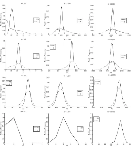
Using the same sample size for these two stochastic systems: In this case, we simulated each

stochastic system 10,000 times with a sample size ofN = 100,N= 1,000, andN = 10,000. Figure 7 depicts the histograms of each node for these two stochastic systems withN = 100 (left column),N = 1,000 (middle column) and N = 10,000 (right column) at time point t = 25, and Figure 8 illustrates these histograms at t = 50. We observe from these two figures that the histograms for each of the stochastic systems do not match well except for in the case of X4, which is probably because the delay only occurs from node 1

to node 2, and hence it has less effect on X4 than on all the other nodes due to the movement from one

node to the next occurring only in the forward direction. Specifically, it is seen that for all the sample sizes investigated, the histogram plots ofX1, X2, X3 obtained for the constructed stochastic system (16) appear

more dispersed than those for the stochastic system with a random delay, and this is especially obvious for

X1 andX2. As we remarked earlier that individuals in the same node for the constructed stochastic system

(16) may be treated differently, while individuals for the stochastic system with a random delay are treated the same. This means that the constructed stochastic system is more “random” than the stochastic system with a random delay, and thus it shows more variation. Figures 7 and 8 also reveal that the histogram plots ofX1, X2, X3obtained for the stochastic system with a random delay are symmetric for all the sample sizes

(18)

0 10 20 30 40 50 60 0 0.02 0.04 0.06 0.08 0.1 0.12 0.14 0.16

N = 100

X1

Relative Frequency

RD C

0 50 100 150 200 250 300 0 0.02 0.04 0.06 0.08 0.1

N = 1,000

X1

Relative Frequency

RD C

6000 800 1000 1200 1400 0.01 0.02 0.03 0.04 0.05 0.06 0.07 0.08

N = 10,000

X1

Relative Frequency

RD C

0 10 20 30 40 50 60 0

0.05 0.1 0.15 0.2

N = 100

X2

Relative Frequency

RD C

1000 150 200 250 300 0.02 0.04 0.06 0.08 0.1 0.12

N = 1,000

X2

Relative Frequency

RD C

20000 2100 2200 2300 2400 2500 0.02

0.04 0.06 0.08 0.1

N = 10,000

X2

Relative Frequency

RD C

30 40 50 60 70 80 0 0.02 0.04 0.06 0.08 0.1 0.12 0.14 0.16

N = 100

X3

Relative Frequency

RD C

6000 620 640 660 680 700 0.02 0.04 0.06 0.08 0.1 0.12

N = 1,000

X3

Relative Frequency

RD C

60000 6100 6200 6300 6400 0.01 0.02 0.03 0.04 0.05 0.06 0.07 0.08 0.09

N = 10,000

X3

Relative Frequency

RD C

0 1 2 3 4

0 0.1 0.2 0.3 0.4 0.5 0.6 0.7

N = 100

X4

Relative Frequency

RD C

0 2 4 6 8 10

0 0.1 0.2 0.3 0.4 0.5 0.6 0.7

N = 1,000

X4

Relative Frequency

RD C

0 10 20 30 40 50 60 0 0.1 0.2 0.3 0.4 0.5 0.6 0.7

N = 10,000

X4

Relative Frequency

RD C

Figure 7: Histograms of the stochastic system with random delays (RD) and the constructed stochastic system (C) with N = 100 (left column), N = 1,000 (middle column), and N = 10,000 (right column) at

(19)

0 10 20 30 40 50 60 0 0.02 0.04 0.06 0.08 0.1 0.12 0.14 0.16

N = 100

X1

Relative Frequency

RD C

0 50 100 150 200 250 300 0 0.02 0.04 0.06 0.08 0.1 0.12

N = 1,000

X1

Relative Frequency

RD C

4000 600 800 1000 1200 1400 0.01 0.02 0.03 0.04 0.05 0.06 0.07 0.08 0.09

N = 10,000

X1

Relative Frequency

RD C

0 10 20 30 40 50 60 0

0.05 0.1 0.15 0.2

N = 100

X2

Relative Frequency

RD C

1000 150 200 250 300 0.02 0.04 0.06 0.08 0.1 0.12 0.14

N = 1,000

X2

Relative Frequency

RD C

19000 2000 2100 2200 2300 2400 2500 0.02 0.04 0.06 0.08 0.1 0.12

N = 10,000

X2

Relative Frequency

RD C

30 40 50 60 70 80 0 0.02 0.04 0.06 0.08 0.1 0.12 0.14 0.16 0.18

N = 100

X3

Relative Frequency

RD C

6000 620 640 660 680 700 0.02 0.04 0.06 0.08 0.1 0.12

N = 1,000

X3

Relative Frequency

RD C

64500 6500 6550 6600 6650 6700 0.01 0.02 0.03 0.04 0.05 0.06 0.07 0.08 0.09

N = 10,000

X3

Relative Frequency

RD C

0 1 2 3 4

0 0.1 0.2 0.3 0.4 0.5 0.6 0.7

N = 100

X4

Relative Frequency

RD C

0 2 4 6 8 10

0 0.1 0.2 0.3 0.4 0.5 0.6 0.7

N = 1,000

X4

Relative Frequency

RD C

0 10 20 30 40 50 60 0 0.1 0.2 0.3 0.4 0.5 0.6 0.7

N = 10,000

X4

Relative Frequency

RD C

Figure 8: Histograms of the stochastic system with random delays (RD) and the constructed stochastic system (C) with N = 100 (left column), N = 1,000 (middle column), and N = 10,000 (right column) at

(20)

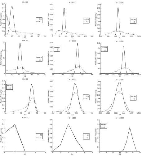
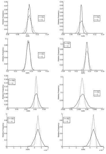
Using different sample size for these two stochastic systems: In Figure 9, we compare the histogram plots obtained from the stochastic system with a random delay for a sample size of N = 10,000 to those obtained from the constructed stochastic system with a sample size ofN= 100,000 and we see that the two histograms are in better agreement for nodes 1 and 2. We offer one possible explanation for this occurrence.

0.060 0.08 0.1 0.12 0.14

0.01 0.02 0.03 0.04 0.05 0.06 0.07 0.08

X1/N

Relative Frequency

RD

C

0.040 0.06 0.08 0.1 0.12 0.14

0.01 0.02 0.03 0.04 0.05 0.06 0.07 0.08 0.09

X1/N

Relative Frequency

RD

C

0.2 0.21 0.22 0.23 0.24 0.25

0 0.02 0.04 0.06 0.08 0.1

X2/N

Relative Frequency

RD C

0.190 0.2 0.21 0.22 0.23 0.24 0.25

0.02 0.04 0.06 0.08 0.1 0.12

X2/N

Relative Frequency

RD C

0.6 0.61 0.62 0.63 0.64

0 0.02 0.04 0.06 0.08 0.1 0.12 0.14 0.16 0.18

X3/N

Relative Frequency

RD

C

0.6450 0.65 0.655 0.66 0.665 0.67

0.05 0.1 0.15 0.2

X3/N

Relative Frequency

RD

C

0 1 2 3 4 5 6

x 10−3

0 0.2 0.4 0.6 0.8 1

X4/N

Relative Frequency

RD

C

0 1 2 3 4 5 6

x 10−3

0 0.2 0.4 0.6 0.8 1

X4/N

Relative Frequency

RD

C

Figure 9: Histograms of the stochastic system with random delays (RD) with a sample size ofN = 10,000 and the constructed stochastic system with a sample size ofN = 100,000 att= 25 (left column) andt= 50 (right column). The histograms are plotted with respect to density.

(21)

deterministic solution at different rates, thus different values for sample size are need to obtain the same order of approximation.

3.6.2 The effect of the variance of a random delay on the comparison of these two stochastic

systems

What remains to be investigated is how the variance of the random delay affects the comparison of the two stochastic systems. However, in order to change the variance, the shape and rate parametersnandαin the probability density functionG(u;α, n) for the random delay must be altered in order to keep the expected value of the random delay to be the same. Specifically, the value ofn determines the number of additional equations to reduce the deterministic system with a distributed delay into a system of ODE’s. Thus, for each additional variance to be considered, a new system of ODE’s and the corresponding stochastic system must be derived.

For the case where n= 10 andα= 2, we have a mean of 5 and a variance of 2.5 for the random delay. Now using the substitutions

cj+4(t) =

Z t

−∞

αj₍_t₋_θ₎j−1

(j−1)! e

−α(t−θ)_κ

1c1(θ)(l2−c2(θ))+dθ, j= 1,2,3, . . . ,10,

we obtain the following system of ODE’s that is equivalent to (13) with delay kernel beingG(u; 2,10)

˙

c2(t) =−κ2c2(t)(l3−c3(t))++c14(t)

˙

c3(t) =−κ3c3(t)(l4−c4(t))++κ2c2(t)(l3−c3(t))+

˙

c5(t) =ακ1c1(t)(l2−c2(t))+−αc5(t)

˙

ci(t) =αci−1−αci fori= 6,7, ...,14

ci(0) =ci0, i= 1,2,3,4

cj+4(0) = Z 0

−∞

αj₍₋_θ₎j−1

(j−1)! e

αθ_κ

1c1(θ)(l2−c2(θ))+dθ, j= 1,2,3, . . . ,10.

We can construct the stochastic system which will converge to this ODE system in the same manner as before. To avoid confusion we will refer to this new stochastic system as the constructed stochastic system withα= 2 to distinguish it from the previously constructed system in which we hadα= 0.2.

The constructed stochastic system withα= 2 was simulated 10,000 times with a sample size ofN= 100 andN = 1,000. The stochastic system with a random delay was simulated for 10,000 trials withN = 100 and N = 1,000, where the random delay has the probability density function G(u;α, n) withn = 10 and

(22)

0 10 20 30 40 50 60 0

0.02 0.04 0.06 0.08 0.1 0.12 0.14

N = 100

X1

Relative Frequency

RD

C

0 50 100 150 200 250 300

0 0.01 0.02 0.03 0.04 0.05 0.06 0.07 0.08 0.09

N = 1,000

X1

Relative Frequency

RD

C

0 10 20 30 40 50 60

0 0.02 0.04 0.06 0.08 0.1 0.12 0.14 0.16 0.18

N = 100

X2

Relative Frequency

RD C

1000 150 200 250 300

0.02 0.04 0.06 0.08 0.1 0.12

N = 1,000

X2

Relative Frequency

RD C

30 40 50 60 70 80

0 0.02 0.04 0.06 0.08 0.1 0.12 0.14 0.16

N = 100

X3

Relative Frequency

RD C

6000 620 640 660 680 700

0.02 0.04 0.06 0.08 0.1

N = 1,000

X3

Relative Frequency

RD

C

0 1 2 3 4

0 0.1 0.2 0.3 0.4 0.5 0.6 0.7

N = 100

X4

Relative Frequency

RD

C

0 2 4 6 8 10

0 0.1 0.2 0.3 0.4 0.5 0.6 0.7

N = 1,000

X4

Relative Frequency

RD

C

(23)

0 10 20 30 40 50 60 0

0.02 0.04 0.06 0.08 0.1 0.12 0.14 0.16

N = 100

X1

Relative Frequency

RD

C

0 50 100 150 200 250 300

0 0.02 0.04 0.06 0.08 0.1 0.12

N = 1,000

X1

Relative Frequency

RD

C

0 10 20 30 40 50 60

0 0.02 0.04 0.06 0.08 0.1 0.12 0.14 0.16 0.18

N = 100

X2

Relative Frequency

RD C

1000 150 200 250 300

0.02 0.04 0.06 0.08 0.1 0.12 0.14

N = 1,000

X2

Relative Frequency

RD C

30 40 50 60 70 80

0 0.02 0.04 0.06 0.08 0.1 0.12 0.14 0.16

N = 100

X3

Relative Frequency

RD C

6000 620 640 660 680 700

0.02 0.04 0.06 0.08 0.1 0.12

N = 1,000

X3

Relative Frequency

RD

C

0 1 2 3 4

0 0.1 0.2 0.3 0.4 0.5 0.6 0.7

N = 100

X4

Relative Frequency

RD

C

0 2 4 6 8 10

0 0.1 0.2 0.3 0.4 0.5 0.6 0.7

N = 1,000

X4

Relative Frequency

RD

C

(24)

4

Comparison Of The Pork Production Model With A Fixed

De-lay And One With A Random DeDe-lay

In this section we compare the pork production model with a fixed delay as in Section 2, to the one with a random delay in Section 3. The value of the delay for the stochastic system with a fixed delay was chosen to be the expected value of the random delay in the stochastic system with a random delay, where the random delay is assumed to be Gamma distributed with probability density functionG(u;α, n) as defined in (14).

For all the simulations below, the model parameter values and initial conditions remain as in Section 2 (Table 1), and the expected value of the random delay is chose to be 5 (i.e., n/α = 5). Each stochastic system was simulated 10,000 times with a sample size of N = 100, N = 1,000, andN = 10,000. For each of the sample sizes, a histogram was constructed for Xi(t), i = 1,2,3,4, att = 25 and t = 50, for each

stochastic system based on these 10,000 sample paths.

4.1

The case with the variance of the random delay

σ

2

= 25

As a first consideration, the variance of the random delay is chosen to be 25.0, that is,n/α2= 25.0. In this case the probability density functionG(u;α, n) for the random delay is chosen such thatn= 1 andα= 0.2. Figure 12 depicts the histograms for these two stochastic systems withN = 100 (left column),N = 1,000 (middle column), andN = 10,000 (right column) att= 25. While Figure 13 illustrates these histograms at

t= 50. We observe from these two figures that the histograms agree well in all cases for nodes 1, 3 and 4, and they agree reasonably well forX2(t) att= 50 for all the sample sizes considered. However, forX2(t) at t= 25 there are larger differences between these two stochastic systems, and the histograms actually deviate increasingly as the sample sizeN is increased. Specifically, the histograms for the stochastic system with a fixed delay was shifted more to the left side as the sample size increases compared to the corresponding ones for the stochastic system with a random delay. But for these cases, the histograms ofX2(t) at t= 25

(25)

0 5 10 15 20 25 0 0.02 0.04 0.06 0.08 0.1 0.12 0.14 0.16

N = 100

X1

Relative Frequency

RD FD

70 80 90 100 110 120 130 140 0 0.02 0.04 0.06 0.08 0.1

N = 1,000

X1

Relative Frequency

RD FD

6000 800 1000 1200 1400 0.01 0.02 0.03 0.04 0.05 0.06 0.07 0.08

N = 10,000

X1

Relative Frequency

RD FD

10 15 20 25 30 35 0

0.05 0.1 0.15 0.2

N = 100

X2

Relative Frequency

RD FD

1800 190 200 210 220 230 240 250 0.02 0.04 0.06 0.08 0.1 0.12

N = 1,000

X2

Relative Frequency

RD FD

20000 2100 2200 2300 2400 2500 0.02

0.04 0.06 0.08 0.1

N = 10,000

X2

Relative Frequency

RD FD

45 50 55 60 65 70 75 0 0.02 0.04 0.06 0.08 0.1 0.12 0.14 0.16

N = 100

X3

Relative Frequency

RD FD

6000 610 620 630 640 650 660 0.02 0.04 0.06 0.08 0.1 0.12

N = 1,000

X3

Relative Frequency

RD FD

62000 6250 6300 6350 6400 6450 0.01 0.02 0.03 0.04 0.05 0.06 0.07 0.08 0.09

N = 10,000

X3

Relative Frequency

RD FD

0 1 2 3 4

0 0.1 0.2 0.3 0.4 0.5 0.6 0.7

N = 100

X4

Relative Frequency

RD FD

0 2 4 6 8 10

0 0.1 0.2 0.3 0.4 0.5 0.6 0.7

N = 1,000

X4

Relative Frequency

RD FD

30 35 40 45 50 55 60 0 0.1 0.2 0.3 0.4 0.5 0.6 0.7

N = 10,000

X4

Relative Frequency

RD FD

(26)

0 5 10 15 20 25 0 0.02 0.04 0.06 0.08 0.1 0.12 0.14 0.16

N = 100

X1

Relative Frequency

RD FD

60 70 80 90 100 110 0 0.02 0.04 0.06 0.08 0.1 0.12

N = 1,000

X1

Relative Frequency

RD FD

7000 750 800 850 900 950 1000 0.01 0.02 0.03 0.04 0.05 0.06 0.07 0.08 0.09

N = 10,000

X1

Relative Frequency

RD FD

10 15 20 25 30 35 0

0.05 0.1 0.15 0.2

N = 100

X2

Relative Frequency

RD FD

2000 210 220 230 240 250 0.02 0.04 0.06 0.08 0.1 0.12 0.14

N = 1,000

X2

Relative Frequency

RD FD

21500 2200 2250 2300 2350 0.02 0.04 0.06 0.08 0.1 0.12

N = 10,000

X2

Relative Frequency

RD FD

45 50 55 60 65 70 75 0 0.02 0.04 0.06 0.08 0.1 0.12 0.14 0.16 0.18

N = 100

X3

Relative Frequency

RD FD

6300 640 650 660 670 680 690 0.02 0.04 0.06 0.08 0.1 0.12

N = 1,000

X3

Relative Frequency

RD FD

64500 6500 6550 6600 6650 6700 0.01 0.02 0.03 0.04 0.05 0.06 0.07 0.08 0.09

N = 10,000

X3

Relative Frequency

RD FD

0 1 2 3 4

0 0.1 0.2 0.3 0.4 0.5 0.6 0.7

N = 100

X4

Relative Frequency

RD FD

0 2 4 6 8 10

0 0.1 0.2 0.3 0.4 0.5 0.6 0.7

N = 1,000

X4

Relative Frequency

RD FD

30 35 40 45 50 55 60 0 0.1 0.2 0.3 0.4 0.5 0.6 0.7

N = 10,000

X4

Relative Frequency

RD FD

(27)

4.2

The case with the variance of the random delay

σ

2

= 2

.

5

Next we considered the case where the probability density functionG(u;α, n) of the random delay is chosen such thatn= 10 andα= 2. The expected value of the delay remains at 5, however the variance is now 2.5, whereas previously the variance was 25.0. Figure 14 depicts the histograms for these two stochastic systems with N = 100 (left column), N = 1,000 (middle column), and N = 10,000 (right column) att = 25. It is

0 5 10 15 20 25

0 0.02 0.04 0.06 0.08 0.1 0.12 0.14

N = 100

X1

Relative Frequency

RD FD

70 80 90 100 110 120 130 140 0 0.02 0.04 0.06 0.08 0.1

N = 1,000

X1

Relative Frequency

RD FD

6000 800 1000 1200 1400 0.01 0.02 0.03 0.04 0.05 0.06 0.07 0.08

N = 10,000

X1

Relative Frequency

RD FD

10 15 20 25 30 35 0 0.02 0.04 0.06 0.08 0.1 0.12 0.14 0.16 0.18

N = 100

X2

Relative Frequency

RD FD

1800 190 200 210 220 230 240 250 0.02 0.04 0.06 0.08 0.1 0.12

N = 1,000

X2

Relative Frequency

RD FD

20000 2100 2200 2300 2400 2500 0.01 0.02 0.03 0.04 0.05 0.06 0.07 0.08 0.09

N = 10,000

X2

Relative Frequency

RD FD

45 50 55 60 65 70 75 0 0.02 0.04 0.06 0.08 0.1 0.12 0.14 0.16

N = 100

X3

Relative Frequency

RD FD

6000 610 620 630 640 650 660 0.02

0.04 0.06 0.08 0.1

N = 1,000

X3

Relative Frequency

RD FD

62000 6250 6300 6350 6400 6450 0.01 0.02 0.03 0.04 0.05 0.06 0.07 0.08 0.09

N = 10,000

X3

Relative Frequency

RD FD

0 1 2 3 4

0 0.1 0.2 0.3 0.4 0.5 0.6 0.7

N = 100

X4

Relative Frequency

RD FD

0 2 4 6 8 10

0 0.1 0.2 0.3 0.4 0.5 0.6 0.7

N = 1,000

X4

Relative Frequency

RD FD

30 35 40 45 50 55 60 0 0.1 0.2 0.3 0.4 0.5 0.6 0.7

N = 10,000

X4

Relative Frequency

RD FD

Figure 14: Histograms of the stochastic system with random delays (RD) and the stochastic system with fixed delays (FD) withN = 100 (left column),N = 1,000 (middle column), andN = 10,000 (right column) att= 25. The random delay was chosen from a Gamma distribution with a mean of 5 and variance of 2.5.

seen from Figure 14 that the histograms for these two stochastic systems agree reasonably well forXi(t),

(28)

t = 25 deviate more as sample size increases, which is obvious for node 1 and more obvious for node 2. Specifically, the histograms of these three nodes obtained for the stochastic system with a fixed delay have similar unimodal shape and dispersion as the corresponding ones obtained for the stochastic system with a random delay, but their mode values become smaller (i.e., shifted more to the left side as compared to the ones obtained for the stochastic system with a random delay) as the sample size increases. Figure 15 depicts the histograms for these two stochastic systems with N = 100 (left column), N = 1,000 (middle column), and N = 10,000 (right column) at t = 50. We observe from this figure that the histograms for

0 5 10 15 20 25

0 0.02 0.04 0.06 0.08 0.1 0.12 0.14 0.16

N = 100

X1

Relative Frequency

RD FD

60 70 80 90 100 110 0 0.02 0.04 0.06 0.08 0.1 0.12

N = 1,000

X1

Relative Frequency

RD FD

7000 750 800 850 900 950 1000 0.01 0.02 0.03 0.04 0.05 0.06 0.07 0.08 0.09

N = 10,000

X1

Relative Frequency

RD FD

10 15 20 25 30 35 0 0.02 0.04 0.06 0.08 0.1 0.12 0.14 0.16 0.18

N = 100

X2

Relative Frequency

RD FD

2000 210 220 230 240 250 0.02 0.04 0.06 0.08 0.1 0.12 0.14

N = 1,000

X2

Relative Frequency

RD FD

21500 2200 2250 2300 2350 0.02

0.04 0.06 0.08 0.1

N = 10,000

X2

Relative Frequency

RD FD

45 50 55 60 65 70 75 0 0.02 0.04 0.06 0.08 0.1 0.12 0.14 0.16

N = 100

X3

Relative Frequency

RD FD

6300 640 650 660 670 680 690 0.02 0.04 0.06 0.08 0.1 0.12

N = 1,000

X3

Relative Frequency

RD FD

64500 6500 6550 6600 6650 6700 0.01 0.02 0.03 0.04 0.05 0.06 0.07 0.08 0.09

N = 10,000

X3

Relative Frequency

RD FD

0 1 2 3 4

0 0.1 0.2 0.3 0.4 0.5 0.6 0.7

N = 100

X4

Relative Frequency

RD FD

0 2 4 6 8 10

0 0.1 0.2 0.3 0.4 0.5 0.6 0.7

N = 1,000

X4

Relative Frequency

RD FD

30 35 40 45 50 55 60 0 0.1 0.2 0.3 0.4 0.5 0.6 0.7

N = 10,000

X4

Relative Frequency

RD FD

(29)

these two stochastic systems agree well for all the four nodes att= 50 for all the sample sizes investigated. Overall, these figures indicate that the histograms for these two stochastic systems agree more compared to the corresponding ones in the previous section (i.e., the case with variance being 25). This is as expected, since as the variance decreases the random delay that is drawn during simulation is forced to be increasingly closer to its mean value. Hence, it is not surprising that the solutions are more similar when there is less variance.

4.3

The case with the variance of the random delay

σ

2

= 0

.

25

(30)

0 5 10 15 20 25 0 0.02 0.04 0.06 0.08 0.1 0.12 0.14

N = 100

X1

Relative Frequency

RD FD

70 80 90 100 110 120 130 140 0 0.02 0.04 0.06 0.08 0.1

N = 1,000

X1

Relative Frequency

RD FD

6000 800 1000 1200 1400 0.01 0.02 0.03 0.04 0.05 0.06 0.07 0.08

N = 10,000

X1

Relative Frequency

RD FD

10 15 20 25 30 35 0 0.02 0.04 0.06 0.08 0.1 0.12 0.14 0.16 0.18

N = 100

X2

Relative Frequency

RD FD

1800 190 200 210 220 230 240 250 0.02 0.04 0.06 0.08 0.1 0.12

N = 1,000

X2

Relative Frequency

RD FD

20000 2100 2200 2300 2400 2500 0.01 0.02 0.03 0.04 0.05 0.06 0.07 0.08 0.09

N = 10,000

X2

Relative Frequency

RD FD

45 50 55 60 65 70 75 0 0.02 0.04 0.06 0.08 0.1 0.12 0.14 0.16

N = 100

X3

Relative Frequency

RD FD

6000 610 620 630 640 650 660 0.02

0.04 0.06 0.08 0.1

N = 1,000

X3

Relative Frequency

RD FD

62000 6250 6300 6350 6400 6450 0.01 0.02 0.03 0.04 0.05 0.06 0.07 0.08 0.09

N = 10,000

X3

Relative Frequency

RD FD

0 1 2 3 4

0 0.1 0.2 0.3 0.4 0.5 0.6 0.7

N = 100

X4

Relative Frequency

RD FD

0 2 4 6 8 10

0 0.1 0.2 0.3 0.4 0.5 0.6 0.7

N = 1,000

X4

Relative Frequency

RD FD

30 35 40 45 50 55 60 0 0.1 0.2 0.3 0.4 0.5 0.6 0.7

N = 10,000

X4

Relative Frequency

RD FD

(31)

0 5 10 15 20 25 0 0.02 0.04 0.06 0.08 0.1 0.12 0.14 0.16

N = 100

X1

Relative Frequency

RD FD

60 70 80 90 100 110 0 0.02 0.04 0.06 0.08 0.1 0.12

N = 1,000

X1

Relative Frequency

RD FD

7000 750 800 850 900 950 1000 0.01 0.02 0.03 0.04 0.05 0.06 0.07 0.08 0.09

N = 10,000

X1

Relative Frequency

RD FD

10 15 20 25 30 35 0 0.02 0.04 0.06 0.08 0.1 0.12 0.14 0.16 0.18

N = 100

X2

Relative Frequency

RD FD

2000 210 220 230 240 250 0.02 0.04 0.06 0.08 0.1 0.12 0.14

N = 1,000

X2

Relative Frequency

RD FD

21500 2200 2250 2300 2350 0.02

0.04 0.06 0.08 0.1

N = 10,000

X2

Relative Frequency

RD FD

45 50 55 60 65 70 75 0 0.02 0.04 0.06 0.08 0.1 0.12 0.14 0.16

N = 100

X3

Relative Frequency

RD FD

6300 640 650 660 670 680 690 0.02 0.04 0.06 0.08 0.1 0.12

N = 1,000

X3

Relative Frequency

RD FD

64500 6500 6550 6600 6650 6700 0.01 0.02 0.03 0.04 0.05 0.06 0.07 0.08 0.09

N = 10,000

X3

Relative Frequency

RD FD

0 1 2 3 4

0 0.1 0.2 0.3 0.4 0.5 0.6 0.7

N = 100

X4

Relative Frequency

RD FD

0 2 4 6 8 10

0 0.1 0.2 0.3 0.4 0.5 0.6 0.7

N = 1,000

X4

Relative Frequency

RD FD

30 35 40 45 50 55 60 0 0.1 0.2 0.3 0.4 0.5 0.6 0.7

N = 10,000

X4

Relative Frequency

RD FD

(32)

5

Conclusions

In this paper we extended the stochastic pork production model in [4] to incorporate delays to account for the phenomenon that movement from one node to the next is often not instantaneous in practice due to the physical distance and/or some unexpected disruptions/interruptions. We considered two different types of delays, a fixed delay and a random delay, and numerically explored the corresponding deterministic approximations for these two resulting stochastic models. Numerical results reveal that when the sample size is sufficiently large the stochastic model with a fixed delay can be well approximated by a system of deterministic differential equations with a fixed delay. This conforms with the recent theoretical results presented in [9]. We also numerically showed that the mean solution of the stochastic model with a Gamma distributed random delay can be well approximated by the solution of a system of deterministic differential equations with a Gamma distributed delay when the sample size is sufficiently large. Hence, the system of deterministic differential equations with a Gamma distributed delay can be used as a possible corresponding deterministic one for this particular stochastic model with a Gamma distributed random delay (with the given parameter values and initial conditions).

In addition, we compared the stochastic model with a Gamma distributed random delay to the stochastic system constructed based on Kurtz’s limit theorem from a system of deterministic differential equations with a Gamma distributed delay. Even though the same system of deterministic differential equations with a Gamma distributed delay can be used as the corresponding deterministic ones for these two stochastic systems, it was found that with the same sample size the histogram plots of the state solutions to the constructed stochastic system are more dispersed than the corresponding ones obtained for the stochastic model with a random delay. However, there is more agreement between the histograms of these two stochastic systems as the variance of the random delay decreases. We also found that with the same variance for the random delay the histogram plots for the stochastic model with a random delay are symmetric for all the sample sizes investigated, while those for the constructed stochastic system are asymmetric when the sample size is small, but become more symmetric as the sample size increases.

Finally we compared the histogram plots of the state solutions to the stochastic model with a fixed delay to those obtained for the stochastic model with a random delay, where the value of the fixed delay is chosen as the mean value of the random delay. Numerical results reveal that for those states most affected by the delay the histogram plots obtained for the stochastic system with a fixed delay have similar unimodal shapes and dispersion as the corresponding ones for the stochastic system with a random delay, but their mode values become smaller (i.e., shifted more to the left side as compared to the corresponding ones obtained for the stochastic system with a random delay) as the sample size increases. We also found that when the variance of the random delay is sufficiently small, the histograms of state solutions to the stochastic model with a fixed delay agree well with the corresponding ones obtained for the stochastic model with a random delay regardless of the sample size.

Acknowledgements

This research was supported in part by Grant Number NIAID R01AI071915-10 from the National Institute of Allergy and Infectious Diseases, in part by the Air Force Office of Scientific Research under grant number AFOSR FA9550-12-1-0188, and in part by the National Science Foundation under Research Training Grant (RTG) DMS-0636590.

References

[1] L.J.S. Allen, An Introduction to Stochastic Processes with Applications to Biology, Chapman & Hall/CRC, Boca Raton, FL, 2011.

[2] D. Anderson, A modified next reaction method for simulating chemical systems with time dependent propensities and delays,The Journal of Chemical Physics, 127(2007), 214107-1–214107-10.

(33)

[4] P. Bai, H.T. Banks, S. Dediu, A.Y. Govan, M. Last, A.L. Lloyd, H.K. Nguyen, M.S. Olufsen, G. Rempala and B.D. Slenning, Stochastic and deterministic models for agricultural production networks, Mathematical Biosciences and Engineering,4(2007), 373–402.

[5] H.T. Banks,