Volume 2007, Article ID 47039,17pages doi:10.1155/2007/47039
Research Article
Higher-Order Statistics for the Detection of Small Objects
in a Noisy Background Application on Sonar Imaging
F. Maussang,1J. Chanussot,2A. H ´etet,3and M. Amate3
1Groupe d’Electromagn´etisme Appliqu´e (GEA), PST Ville d’Avray, Universit´e Paris X-Nanterre, 1 chemin Desvalli`eres,
92410 Ville d’Avray, France
2Laboratoire des images et des signaux (LIS) GIPSA, ´Ecole Nationale Sup´erieure d’Ing´enieurs ´Electriciens de Grenoble,
Institut National Polytechnique de Grenoble (INPG), Domaine Universitaire, BP 46, 38402 Saint-Martin-d’H`eres Cedex, France
3Groupe d’Etudes Sous-Marines de l’Atlantique, DGA/DET/GESMA, BP 42, 29240 Brest Arm´ees, France
Received 21 June 2006; Revised 10 November 2006; Accepted 21 November 2006
Recommended by Christoph Mecklenbr¨auker
An original algorithm for the detection of small objects in a noisy background is proposed. Its application to underwater objects detection by sonar imaging is addressed. This new method is based on the use of higher-order statistics (HOS) that are locally esti-mated on the images. The proposed algorithm is divided into two steps. In a first step, HOS (skewness and kurtosis) are estiesti-mated locally using a square sliding computation window. Small deterministic objects have different statistical properties from the back-ground they are thus highlighted. The influence of the signal-to-noise ratio (SNR) on the results is studied in the case of Gaussian noise. Mathematical expressions of the estimators and of the expected performances are derived and are experimentally confirmed. In a second step, the results are focused by a matched filter using a theoretical model. This enables the precise localization of the regions of interest. The proposed method generalizes to other statistical distributions and we derive the theoretical expressions of the HOS estimators in the case of a Weibull distribution (both when only noise is present or when a small deterministic object is present within the filtering window). This enables the application of the proposed technique to the processing of synthetic aperture sonar data containing underwater mines whose echoes have to be detected and located. Results on real data sets are presented and quantitatively evaluated using receiver operating characteristic (ROC) curves.
Copyright © 2007 F. Maussang et al. This is an open access article distributed under the Creative Commons Attribution License, which permits unrestricted use, distribution, and reproduction in any medium, provided the original work is properly cited.
1. INTRODUCTION
Higher-order statistics (HOS) are largely used in signal pro-cessing and have already been applied to various domains: astronomy (that provided pioneering applications), but also seismic data processing, communication and, more recently, geophysics, speech, radar, and sonar signal processing and analysis. In the last decade, several journals have published
special issues on these emerging techniques [1–3]. As a
mat-ter of fact, HOS allow the solving of problems that first- and second-order statistics fail to solve. For example, they enable
linear system identification by blind deconvolution [4,5],
and nonlinear identification (Volterra filter) [6]. They are
used in nonstationary signals analysis [7], array processing
[8], and source separation [9–11].
A much scarcer literature addresses the use of HOS in the field of image processing (considering images as
bidi-mensional signals). Jacovitti [12] presented applications of
HOS to image decomposition, blind deconvolution, coding and pattern recognition. Some studies were also made on
texture analysis [13,14] and segmentation by data clustering
[15]. Carrato and Ramponi [16] presented a
Skewness-of-Gaussian edge extractor applied on images. This method uses the crossing of a skewness operator by zero (corresponding to a symmetric distribution) to detect edges in images with
good performances and robustness [17]. The most
interest-ing paper regardinterest-ing our application is proposed by
Alexan-drou et al. [18]: a coefficient of excess, the kurtosis
(4th-order statistical value), is studied in (4th-order to model the non-Gaussian reverberation hypothesis. But, as raised by the
au-thors, it is difficult to differentiate this excess, induced by an
inaccurate modeling of the background with a Gaussian law, from a potential coherent component embedded in the
re-verberation. Moreover, this difficulty increases as the number
In this paper,1a new statistical detection method on
im-ages is proposed. It aims at detecting small targets, modeled as deterministic regions, in a noisy background which is pre-viously statistically modeled by a Weibull law. It is based on higher-order statistical properties of the image. The global detection process can be divided into four main steps:
(1) HOS (skewness or kurtosis) are locally estimated on a square computation window sliding all over the image; (2) the results are focused with a matched filter in order to
accurately locate the sought regions;
(3) a rebuilding of the sought regions is performed using a morphological dilation;
(4) finally, a gray-level threshold is applied to detect the objects (ROC curves).
The paper is organized as follows. In Section 2, some
properties of the used HOS are recalled and two classical esti-mators (for the skewness and the kurtosis, resp.) are defined
and presented. InSection 3, the use of HOS for the purpose
of detection is discussed in function of the signal-to-noise
ra-tio (SNR). InSection 4, the focusing process used in order to
obtain an accurate localization of the different regions of
in-terest is presented. In the last section, the proposed method is tested on real sonar data containing various underwater objects, both lying on the sea-bed and buried, after a presen-tation of the statistical specificities of these images. In partic-ular, this requires the derivation of the theoretical HOS esti-mators in the case of a Weibull distribution.
2. HOS ESTIMATORS
2.1. Definitions
The two most classically used HOS are the skewness (derived from the 3rd-order moment) and the kurtosis (derived from
the 4th-order moment) [19]. One should underline that
be-yond these two standard statistics, other statistics with an or-der greater than 4 can be mathematically defined. However,
these statistics are extremely difficult to estimate in a reliable
and robust way and are thus practically never used. Noting
μX(r)as therth order central moment of a random variable
X, the definition of the skewness is given by
SX=μX(3) μ3/2
X(2)
. (1)
A definition of the kurtosis is given by
KX=μX(4) μ2X(2)
−3. (2)
The skewness measures the symmetry of a random tion, while the kurtosis measures whether the data distribu-tion is peaked or flat relative to a normal distribudistribu-tion. These statistics are theoretically null for the normal distribution.
1This paper is on results obtained by F. Maussang during his Ph.D. in LIS.
2.2. Estimators
To estimate the skewness and the kurtosis on a sampleXof
finite sizeN,k-statistics kX(r) can be used. kr is defined as
the unique symmetric unbiased estimator of the cumulant
κX(r) on X [19]. An unbiased estimator of the skewness is
then given by
SX=kX(3) kX3/(2)2
. (3)
Defining therth sample central moment ofXby the
follow-ing expression:
mX(r)=
1 N
N
i=1
xi−x
r
, (4)
wherex =(1/N)Ni=1xiandxiare theNsamples ofX, we
can derive another definition of this estimator. Actually,
con-sidering the relationships betweenkX(r)andmX(r), we have
SX=
N(N−1) N−2
mX(3)
m3/2
X(2)
. (5)
In the same way, we derive the following estimator for the kurtosis:
KX=kX(4) k2
X(2)
= (N+ 1)(N−1)
(N−2)(N−3)
mX(4)
m2
X(2)
− 3(N−1)2
(N−2)(N−3).
(6)
Asymptotic statistical properties are studied for high values
of N. Firstly, we can mention that these estimators are
bi-ased in the first order and that they are correlated (the bias being dependent on higher-order moments). However, ex-act results can be derived in the Gaussian case. In this case,
MandVbeing, respectively, the mean and the variance, we
have
MSX
=0, M KX
=0,
VSX
= 6N(N−1)
(N−2)(N+ 1)(N+ 3) ≈
6 N,
V KX
= 24N(N−1)2
(N−3)(N−2)(N+ 3)(N+ 5)≈
24 N.
(7)
In the general case, there is no analytical expression for un-biased estimators independently from the probability density function of the random value. However, one should note that in the case of a normal distribution, the estimators are unbi-ased. Nevertheless, variances of these estimators are relatively high and it is well known that a reliable estimation requires a large set of samples.
3. HOS FOR DETECTION
To illustrate the detection method proposed in this paper, it
It consists of a square of size 11×11, with a constant
ampli-tudeA, surrounded by a noisy background. The noise in this
image has a central Gaussian distribution with a varianceσ2
B. Its probability density function is given by
GB(B)= 1 σB
√
2πexp
− B2
2σ2
B
(8)
and itsrth noncentral momentsμB(r)are
μB(r)=
⎧ ⎪ ⎨ ⎪ ⎩
σr
B r
!
(r/2)!2r/2 ifris even,
0 otherwise.
(9)
Note that combining these noncentral moments leads to the nullity of the skewness and kurtosis for a normal distribu-tion.
Regarding the deterministic square of amplitudeA, its
rth noncentral momentsμD(r)are
μD(r)=Ar. (10)
Considering the deterministic square as a signal surrounded by noise, the SNR can be defined as
ρ= A σB
(11)
and in decibels:
ρdB=10 log10
A2
σ2
B
=20 log10(ρ). (12)
Skewness and kurtosis are invariant by a scale shift. This is of the utmost importance: since, in the following, the HOS are estimated locally, the proposed method is invariant to
vary-ing offset in the image. Consequently, if the noise is
mod-eled by a noncentral Gaussian of mean μand varianceσ2,
described by the following density probability function:
GB(B)= 1 σB
√
2πexp
−(B−μ)2
2σB2
(13)
all the results obtained in the following remain valid with an SNR defined as
ρ=|A−μ| σB .
(14)
3.1. Local properties of the HOS
Skewness and kurtosis estimators previously described in (5)
and (6) are used in this paper to detect small deterministic
regions in a noisy image. For this purpose, these HOS are lo-cally estimated for each pixel using a square sliding window,
composed ofNpixels, the current pixel being in the center.
To model the situation and explain the results obtained
when applied on the images,p∈[0, 1] is defined as the
pro-portion of deterministic pixels in the computation window (Figure 1). Consequently, (1−p) is the proportion of random
a d
c
b
Figure1: Various values of parameterp: (a)p=0, (b)p=1/9, (c) p=2/9, (d)p=1 (black pixels=deterministic region, white pixels
=background).
values (pixels belonging to the noisy background). In the fol-lowing, the local statistical properties (moments) of the de-terministic region and the noisy background in the compu-tation window are assumed to be the same as the global ones presented in the previous section. This is achieved when the size of the computation window is large enough. In particu-lar, this size should be greater than the maximum size of the sought deterministic regions. Note that in practical cases, the
value ofpfor one given position of course remains unknown.
Considering μD(r), μB(r), and μW(r) the rth noncentral
moments computed on the “deterministic-part” of the fil-tering window, on the “noisy background part,” and on the whole window, respectively, the following relation holds:
μW(r)=p·μD(r)+ (1−p)·μB(r). (15)
Therefore, we can combine the definitions of the skewness
and kurtosis in (1) and (2), the noncentral moments of the
different parts of the window in (9) and (10), the definition
of the SNRρ(11), and the relationships between the central
and noncentral moments [19]. Using the previous model, we
derive the following expressions for the skewnessSWand the
kurtosisKWestimated on the computation window:
SW(ρ,p)= p
1−p
(1−2p)ρ3−3ρ
pρ2+ 13/2 ,
KW(ρ,p)= 1−p p
1−6p+ 6p2ρ4−6(1−2p)ρ2+ 3
pρ2+ 12 .
(16)
The evolution of these HOS in function of pand the SNRρ
is plotted onFigure 2. Different behaviors are observed
de-pending on whether the SNR is high or low. The skewness has low values for low SNRs, but, for high SNRs, it has high
values for low values ofpand negative values for high values
of p(close to 1). This is confirmed byFigure 3(a)where we
can observe the skewness getting close to zero for low SNRs
(below 0 dB for lowpand below−20 dB for highp) and
tak-ing higher values for high SNRs (above 20 dB). Intermediate values are obtained for intermediate values of the SNR. For
the kurtosis (Figure 3(b)), opposed behaviors are observed
10 5 0 5 10
Sk
ew
ness
100 50
0 50
100
SNR (dB)
0
0.5
1
Deterministic
proportion
p
6 4 2 0 2 4 6 8
(a) Skewness
20 0 20 40 60 80 100
Ku
rt
o
si
s
100 50
0 50
100
SNR (dB)
0
0.5
1
Deterministic
proportion
p
0 10 20 30 40 50 60 70 80 90
(b) Kurtosis
Figure2: HOS in function of the deterministic proportionpand the SNR.
8 6 4 2 0 2 4 6 8 10
Sk
ew
ness
100 50 0 50 100
SNR (dB) p=0.01
p=0.95
(a) Skewness
20 0 20 40 60 80 100
Ku
rt
o
si
s
100 50 0 50 100
SNR (dB) p=0.01
p=0.95
(b) Kurtosis
Figure3: HOS in function of the SNR for lowp(solid line) or highp(dashed line).
sections in the case of low, high, and intermediate SNRs, re-spectively.
3.2. Application to small objects detection:
the case of low SNRs
In this section, we consider images containing small objects (target, fault, and other manmade or natural objects mod-eled as small deterministic regions), with a low SNR as men-tioned in the previous section and derived from the curves
presented on Figure 3. SNRs lower than −20 dB are
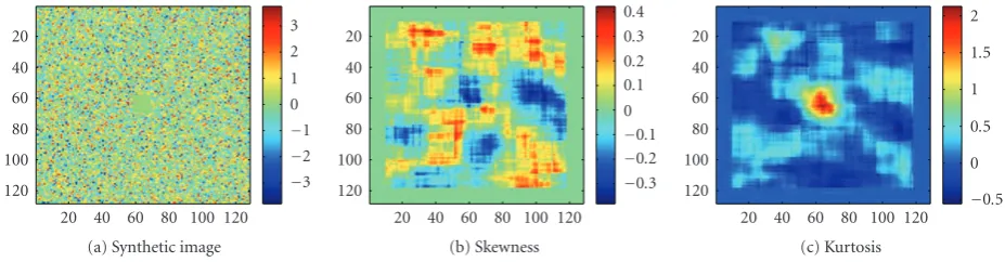
con-sidered as low SNRs. For an illustrative purpose, HOS are
estimated in a synthetic image as previously described with
an SNR of−60 dB (Figure 6(a)).
For low SNRs, we derive the following approximate ex-pressions of the equations presented in the previous section
(16):
SW(p)≈lim
ρ→0SW(ρ,p)=0,
KW(p)≈lim
ρ→0KW(ρ,p)=
3p
1−p.
(17)
These approximations are confirmed byFigure 4where, for
50 0 50 100
HOS
value
0 0.2 0.4 0.6 0.8 1
Deterministic proportionp Skewness
Kurtosis
Figure4: Skewness (dashed line) and kurtosis (solid line) in func-tion of parameterpfor SNR= −60 dB.
whenpgoes from zero to one, and the skewness values are
close to zero. This result is illustrated onFigure 5,
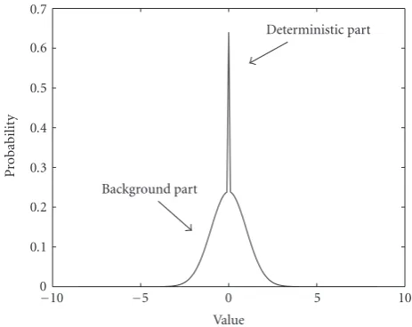
represent-ing an example of probability density function obtained on a window with a low SNR, showing a symmetric density, hence a low skewness, with a peak, hence a high kurtosis.
These approximations also explain the results obtained
with the synthetic image (Figure 6). Note that on this
exam-ple only used for illustration, the detection would be trivial since the “target” is clearly visible. However, we must under-line that in real cases the regions of interest can be composed of a very few pixels in a very large image, thus with an ex-tremely low visibility.
The skewness image (Figure 6(b)) only consists of low
values, without any clearly contrasted region emerging from the noisy background. On the contrary, the kurtosis has low values in the regions corresponding to the noisy background and higher values around the center of the deterministic re-gion. This is consistent with the predicted increase of the
kur-tosis withp. Actually, the closer is the filtering window to the
center of the object, the higher is the deterministic
propor-tionpin the window. Note that the previous approximations
remain valid when no deterministic region is present (e.g.,
in the noisy background, withp=0). Therefore, in the case
of low SNRs, a detection of small deterministic objects can be made by performing a simple threshold selecting the high values of the kurtosis. On the other hand, skewness does not lead to any satisfactory detection.
Given the influence ofpon the kurtosis, the smaller is the
computation window, the higher are the values of the kur-tosis, and the better is the detection. This is illustrated on Figure 7where we can see higher and more centered values
of the kurtosis with a 13×13 window than with a 41×41 one.
But, as stated inSection 2.2(7), the smaller is this window,
the higher is the variance of the estimator, and the less robust
0 0.1 0.2 0.3 0.4 0.5 0.6 0.7
P
robabilit
y
10 5 0 5 10
Value Background part
Deterministic part
Figure5: Example of probability density function on a computa-tion window for a low SNR (p=0.4).
is the detection. This is illustrated onFigure 7(a)where the
maximum is about 8.2 when the theoretical result predicts
pmax =11×11/13×13 =121/169 which leads to a
maxi-mum value of 3pmax/(1−pmax)≈7.56 for the kurtosis.
To illustrate these comments, two numerical values are computed on the results. The first one is the variance of the HOS on the background (to the exclusion of all the pixels where the filtering window actually meets the target). The second criterion measures the contrast: it is the ratio be-tween the maximum value of the HOS on the image (ab-solute value) and the standard deviation of the background (square root of the variance previously estimated). This pa-rameter allows to estimate the quality of the detection, bound with the enhancement of the regions of interest compared
with the background.Table 1presents the results obtained on
the HOS images with an SNR of−60 dB and different sizes
of computation window.
As previously mentioned, the narrower is the computa-tion window (and the lower is the number of samples), the higher are the variances of the HOS estimators. This induces an increase of the variance of the background. This is even
higher for the kurtosis, as predicted by (7) (with a ratio close
to 4, especially for large windows). However all the variances are significantly lower than the variance of the original image (close to 1, the Gaussian noise being of standard deviation 1). Furthermore, the contrast values confirm our previous visual observations regarding the kurtosis: the detection is easier for small computation windows. Regarding the skew-ness, the contrast has lower values, whatever the size of the window, confirming its low potential in terms of detection.
To conclude with the detection in the case of a low SNRs, the skewness is of little interest, its values always being close to zero, whether there is an object or not. On the contrary, the kurtosis gives interesting results for the detection. However,
a trade-offhas to be found for the size of the computation
120 100 80 60 40 20
20 40 60 80 100 120 3 2 1 0 1 2 3
(a) Synthetic image
120 100 80 60 40 20
20 40 60 80 100 120
0.3 0.2 0.1 0 0.1 0.2 0.3 0.4
(b) Skewness
120 100 80 60 40 20
20 40 60 80 100 120
0.5 0 0.5 1 1.5 2
(c) Kurtosis
Figure6: HOS evaluated on 21×21 windows (SNR= −60 dB).
120 100 80 60 40 20
20 40 60 80 100 120 0 1 2 3 4 5 6 7 8
(a) 13×13
120 100 80 60 40 20
20 40 60 80 100 120
0.5 0 0.5 1 1.5 2
(b) 21×21
120 100 80 60 40 20
20 40 60 80 100 120
0.1 0 0.1 0.2 0.3 0.4 0.5
(c) 41×41
Figure7: Kurtosis images obtained with different sizes of window (SNR= −60 dB).
Table1: Detection performances of the HOS (variance of the back-ground and contrast), with an SNR of−60 dB, in function of the size of the computation window.
Size of the window Skewness Kurtosis Variance Contrast Variance Contrast 13×13 0.0282 7.94 0.115 24.6 21×21 0.0099 4.23 0.0375 11.0 41×41 0.0011 5.42 0.0039 8.99
kurtosis, and thus a better detection, but with a high variance of estimation.
3.3. Application to the detection of small objects:
the case of high SNRs
In this section, we consider images containing small objects
with a high SNR. As suggested by the curves on Figure 3,
SNRs greater than 40 dB are considered as high SNRs. For an illustrative purpose, HOS are estimated in a synthetic image
with a 50 dB SNR (Figure 9(a)).
For high SNRs (ρ→ ∞), we derive the following
approxi-mate expressions of the previously presented equations (16):
SW(p)≈ρlim→+∞SW(ρ,p)=
1−2p
p(1−p), (18)
KW(p)≈ρ→+∞lim KW(ρ,p)=
1−6p+ 6p2
p(1−p) . (19)
10 5 0 5 10 15 20
HOS
value
0 0.2 0.4 0.6 0.8 1
Deterministic proportionp Skewness
Kurtosis
Figure 8: Skewness (dashed line) and kurtosis (solid line) for SNR=50 dB.
This is illustrated onFigure 8. For an SNR of 50 dB: the
kur-tosis decreases from infinity to−2 when pincreases from 0
to 0.5. It again increases to infinity when pincreases from
120 100 80 60 40 20
20 40 60 80 100 120 0 50 100 150 200 250 300
(a) Synthetic image
120 100 80 60 40 20
20 40 60 80 100 120 0 50 100 150 200 250 300 350 400
(b) Skewness
120 100 80 60 40 20
20 40 60 80 100 120 0 50 100 150 200 250 300 350 400
(c) Kurtosis
Figure9: HOS evaluated on 21×21 windows (SNR=50 dB).
120 100 80 60 40 20
20 40 60 80 100 120 0 20 40 60 80 100 120 140 160
(a) 13×13
120 100 80 60 40 20
20 40 60 80 100 120 0 50 100 150 200 250 300 350 400
(b) 21×21
120 100 80 60 40 20
20 40 60 80 100 120 0 200 400 600 800 1000 1200 1400 1600
(c) 41×41
Figure10: Kurtosis images obtained with different sizes of window (SNR=50 dB).
from plus to minus infinity aspgoes from 0 to 1, with a zero
crossing forp=0.5.
Figure 9illustrates this situation and presents the results
obtained for the skewness and the kurtosis (Figures9(b)and
9(c), resp.) in the case of a synthetic test image with a high
SNR (Figure 9(a)). We can make the following observations.
(i) In a noisy background, the HOS have small values. This corresponds to the nullity of the HOS for the Gaussian distribution (note that in this specific case, the
approxima-tions proposed in (18) and (19) do not hold anymore).
(ii) Square structures are observed around the object of interest. They are composed of pixels with high values, the highest being in the corners.
The size of these squares corresponds to the size of the deterministic region plus the size of the computation win-dow. Considering the deterministic region as a square of side
nD and a square computation window of sidenW (the
to-tal number of pixels inside the computation window being N = n2
D), the sidenS of the square appearing in the HOS
images is given by
nS=nD+nW−1. (20)
For example, onFigure 9, the object is of size 11×11. This
leads to a 31×31 frame.
As seen onFigure 8, the estimators reach their maximal
values for the minimal values of parameter p. This
corre-sponds to the case where one single pixel of the object of interest is included in the computation window (i.e., the cor-ner of the structure, when the computation window starts
overlapping it). When the number of deterministic pixels in-cluded inside the filtering window increases (i.e., when the window keeps on sliding towards the center of the object), the value of the estimators decreases. That explains the shape of the square structures observed in the result images and the decreasing values along the edges and inside the square.
From (18) and (19), for low values ofp, skewness can be
ap-proximated by 1/√pand kurtosis by 1/ p. This explains that
for a 21×21 window, the highest values in the skewness
im-age is close to 21 (corresponding to p = 1/(21×21)) and
441 for the kurtosis. As a consequence, the higher is the size of the computation window, the higher is the value of the
maximum on the skewness and the kurtosis image.Figure 10
illustrates the effect of the size of the computation window
on the kurtosis estimation results: the larger is the window, the larger is the resulting square and the higher is the
max-imum value (check the scales). Whenpgoes above 0.5 (the
computation window contains more pixels belonging to the deterministic object than to the noisy background), the kur-tosis starts to increase again, which explains increasing
val-ues near the center of the sought region onFigure 10(a). To
120 100 80 60 40 20
20 40 60 80 100 120 0 500 1000 1500 2000 2500 3000
(a) Synthetic image
120 100 80 60 40 20
20 40 60 80 100 120 0 100 200 300 400 500 600 700 800 900
(b) 31×31
120 100 80 60 40 20
20 40 60 80 100 120 0 20 40 60 80 100 120 140 160 180 200
(c) 15×15
Figure11: Kurtosis images obtained with different sizes of window on a synthetic image with two regions (left object: SNR=70 dB, right object: SNR=50 dB).
size of the deterministic region plus the size of the compu-tation window. If one given image contains several objects of interest, the corresponding structures in the HOS images may overlap if the filtering window is too large. This
situ-ation is illustrated onFigure 11with two regions of diff
er-ent amplitudes and different sizes (5×5 on the left, 11×11
on the right), with a 21 pixel wide gap in between. Note on Figure 11(b)the independence of the kurtosis value from the SNR (both objects lead to the same maximum value).
The contrasts reported onTable 2confirm these
obser-vations, the contrast increasing with the size of the compu-tation window. The variances being estimated on the noisy
background, the variances reported onTable 1 do not
de-pend on the SNR. The contrast estimated on the original image corresponds to the SNR (about 316.2 for 50 dB). The contrast obtained with the HOS is largely greater, especially for a large window. This highlights the interest of a detection using these statistical values. Finally, note that, for a given size of window, the contrast obtained with the kurtosis is greater than with the skewness. This is also confirmed by the derived approximations that give higher values of the kurtosis for low
values of p(lower than approximately 0.15, (2−√2)/4
ex-actly).
As a conclusion to this section, both the skewness and the kurtosis allow the detection of deterministic regions. How-ever, the maximum values being in the corners of a square located around the region of interest, the precise localization of the sought regions requires some post processing. This “focusing” of the resulting frames to the real position of the
objects will be studied inSection 4. Moreover, the choice of
the size of the computation window appears as a trade-off
between the size of the deterministic regions that must be
detected and the space separating two different objects.
3.4. Application to the detection of small objects:
the case of intermediate SNRs
SNRs between −20 dB and 40 dB are considered as
inter-mediate SNRs. As we can see on Figure 3, detection
per-formances are still interesting for these SNRs, but they be-come more complex to evaluate and understand. Whereas
Table2: Detection performances of the HOS (contrast), with an SNR of 50 dB, in function of the size of the computation window.
Window size Contrasts
Skewness Kurtosis
13×13 77.3 496.2
21×21 209.4 2270.9 41×41 1195.4 2.59×10⁴
skewness values remain close to zero for SNRs below 10 dB
for small values of p, negative values with high amplitude
appear for SNRs greater than−50 dB, with a peak at 0 dB,
for high values ofp. Therefore, for an SNR between−50 dB
and 10 dB, a detection is possible by isolating pixels leading to a negative skewness. They are located close to the
cen-ter of the decen-terministic region (seeFigure 12(b)). For higher
SNRs (greater than 10 dB), the skewness increases regularly to reach the approximations obtained for high SNRs. For such SNRs, square structures are observed as previously
de-scribed (see Figures 9(b)and13(b)), the values decreasing
more slowly near the center, but with the same structure as with high SNRs. In this case the detection method is the same as for high SNRs.
The kurtosis behaves similarly to the low SNRs case un-til approximately 10 dB with a value progressively
decreas-ing for high values ofp(Figure 3(b)). The detection is
possi-ble by selecting the highest values in the kurtosis image: they
are located near the center of the object (Figure 12(c)). This
is similar to the low SNRs case (Figure 7(a)), but the
con-trast between the highest kurtosis values and the noisy back-ground is smaller. For higher SNRs (greater than 10 dB), the
kurtosis increases progressively for low values ofp, reaching
the approximations derived for high SNRs. As previously
de-scribed, square frames appear (Figure 13(c)), the values
de-creasing more slowly near the center, but with the same struc-ture as with high SNRs. Again, the detection method is the same as for high SNRs.
The numerical values reported in Tables 3 and4
120 100 80 60 40 20
20 40 60 80 100 120 3 2 1 0 1 2 3
(a) Synthetic image
120 100 80 60 40 20
20 40 60 80 100 120 2 1.5 1 0.5 0 0.5
(b) Skewness
120 100 80 60 40 20
20 40 60 80 100 120 0 1 2 3 4 5 6
(c) Kurtosis
Figure12: HOS evaluated on 13×13 windows (SNR=0 dB).
120 100 80 60 40 20
20 40 60 80 100 120 2 0 2 4 6 8 10
(a) Synthetic image
120 100 80 60 40 20
20 40 60 80 100 120 0 0.5 1 1.5 2 2.5 3 3.5
(b) Skewness
120 100 80 60 40 20
20 40 60 80 100 120 0 5 10 15 20 25
(c) Kurtosis
Figure13: HOS evaluated on 21×21 windows (SNR=20 dB).
Table3: Detection performances of the HOS (contrast), with an SNR of 0 dB, in function of the size of the computation window.
Window size Contrasts
Skewness Kurtosis
13×13 14.5 19.9
21×21 8.39 4.46
41×41 6.84 5.21
contrasts are lower than in the previous case, but they still remain largely above the SNR of the original image.
4. DETECTION WITH HIGH SNRs: FOCUSING OF THE RESULTS
4.1. Matched filtering approach
In the case of high SNRs, square frames appear around the deterministic regions in the skewness and the kurtosis images, the highest values being in the corner of these struc-tures. This does not allow the correct localization of the sought elements in the image. To solve this problem, a matched filtering approach is proposed in this section by per-forming a correlation of the HOS image with a theoretical
Table4: Detection performances of the HOS (contrast), with an SNR of 20 dB, in function of the size of the computation window.
Window size Contrasts
Skewness Kurtosis
13×13 24.4 75.5
21×21 38.8 131.3
41×41 113.3 384.5
model of the result. The results of this focusing will only be presented on the kurtosis image, the results obtained with the skewness being similar with the corresponding theoreti-cal model.
Knowing the size of the computation window and ap-proximately knowing the size of the sought objects, the
approximation presented in (19) is used to build a
suit-able model. For example, for the kurtosis image obtained onFigure 15(a), the obtained model is shown onFigure 14
(with a size of 31×31 as explained by (20)). We can see
100 0 100 200 300 400 500
A
m
plitude
40 30
20 10
0 0 10 20
30 40 0 50 100 150 200 250 300 350 400
Figure14: Kurtosis theoretical model used for the matched filter (window size 21×21, region size 11×11).
4.2. Uncertainty regarding the size of
the deterministic region
The size of the used computation window is known (it is user-defined), but the size of the sought objects is not pre-cisely known. As a consequence, the sizes of the structures needing to be focused in the HOS images remain partially unknown. A solution consists in taking, for the correlation,
a model built with the sum of several models with different
sizes. This sum is weighted in accordance with a Gaussian distribution with a mean corresponding to the most typical size, and a variance bound with the incertitude on the knowl-edge of this size. It is tested on an image containing two
de-terministic regions (Figure 11(a), described inSection 3.3).
If a 25×25 model is chosen on the kurtosis image obtained
with a 15×15 window (Figure 16(a)), only the wider region
is correctly focused (Figure 16(b)). To solve this problem, a
new model is built with a mean size of 23×23 and an
uncer-tainty (standard deviation of the Gaussian distribution) of 3 (Figure 17). This allows a fairly good detection of the two
regions (Figure 16(c)).
4.3. Rebuilding of the region of interest:
dilation with a fuzzy operator
The focusing of the HOS results allows to have the highest values in the center of the sought region. This is very inter-esting for detection and localization of the region, but it does not give its shape and size. A morphological dilation is per-formed on the focused HOS images to solve this problem.
The operator use is fuzzy [20] in order to take into account
the uncertainty on the size of the sought region. The model uses the same size of uncertainty as for the matched filter.
The corresponding results are presented inSection 5.2.
A simple threshold of the latter image then allows an easy detection and precise localization of the sought regions. If available, further prior knowledge about the characteristics
of the object of interest can be incorporated into the model (e.g., a rectangular shape can be used instead of a square).
5. APPLICATION IN SONAR IMAGING
In this section, the proposed algorithm is tested on real sonar images, with application to underwater mines detec-tion. These images are obtained by a synthetic aperture sonar (SAS), an active sonar imaging system providing high reso-lution images of the sea bed.
5.1. Specificities in sonar imaging
The sonar images used in this section represent the sea bed
with different objects lying, partially or completely buried
in the sea floor. When they are not buried, the objects cast a shadow on the sea bed (see, e.g., the triangular shaped
shadow onFigure 19(a)). All these objects also generate some
echoes (reflexion of the sound wave on the objects), these echoes being the only noticeable element in the case of buried
objects. As seen on Figures20(a)and21(a), these objects are
hardly visible and the images are seriously corrupted by a speckle noise giving a granular aspect to the image and dis-turbing its interpretation.
A good statistical model of this noise in the case of high resolution images is given by the Weibull law described by
the following probability density function [21,22]:
WB(B)=δ α
B α
δ−1
exp
−
B α
δ
, B≥0, (21)
withαthe scale parameter andδthe shape parameter, strictly
positive.
With such a non-Gaussian distribution, background
val-ues of the skewnessSBand the kurtosisKBare not null
any-more (see the appendix). On real SAS data,δis function of
the resolution of the image, but it is generally approximated
by 1.65 [23]. This corresponds to skewness and kurtosis
val-ues close to 1 (Figure 18).
Considering the echoes generated by the mines as
deter-ministic elements of amplitudeA, the SNR is defined as
ρW =A
α. (22)
This assumption is simple but fair, since the echoes are gener-ally composed of a few pixels, with values included in a
lim-ited range compared to the background (it would be difficult
to model these values with a random distribution).
The approximations made inSection 3.3remain valid in
the case of high SNRs. As a matter of fact, the resulting coeffi
-cients of the highest orders (3 for the skewness, 4 for the kur-tosis) are the same (see the terms in bold in the appendix). This induces similar detection properties with the previous case. For sonar images, the SNR as defined above is far greater than 0 dB, even in the case of buried objects. As a conclusion,
following the discussions inSection 3on detection in the case
of high or intermediate SNRs, the proposed algorithm is well
120 100 80 60 40 20
20 40 60 80 100 120 0 50 100 150 200 250 300 350 400
(a) Kurtosis image.
120 100 80 60 40 20
20 40 60 80 100 120 5 10 15 20 25 30 35 40 45 50 55
(b) Matched filtering.
70 65 60 55 50 45 40 35
35 40 45 50 55 60 65 70 5 10 15 20 25 30 35 40 45 50 55
(c) Zoom.
Figure15: Matched filtering on the kurtosis image (window size 21×21).
120 100 80 60 40 20
20 40 60 80 100 120 0 20 40 60 80 100 120 140 160 180 200
(a) Kurtosis image (15×15).
120 100 80 60 40 20
20 40 60 80 100 120 5 10 15 20 25 30
(b) Matched filtering with no uncer-tainty.
120 100 80 60 40 20
20 40 60 80 100 120 1 2 3 4 5 6 7 8
(c) Matched filtering with uncer-tainty.
Figure16: Matched filtering on the kurtosis image of two deterministic regions with no uncertainty (25×25) and an uncertainty (23×23, SD=3).
20 0 20 40 60 80
40 30
20 10
0 0 10 20
30 40 0 10 20 30 40 50 60
Figure17: Kurtosis theoretical model used for the matched filter (mean window size 23×23, SD=3).
5.2. Results on SAS images
In this section, the proposed detection method is tested on various real SAS images provided by the DGA (D´el´egation G´en´erale de l’Armement, France). The resolution is defined
here as the size of one pixel. This is different from the actual
0 1 2 3 4 5 6
Bac
k
gr
ound
HOS
val
ue
1 1.2 1.4 1.6 1.8 2
δ
Skewness Kurtosis
Figure18: Weibull background HOS values in function of the pa-rameterδ.
6 5.5 5 4.5 4 3.5
Az
imut
h
(m
)
6 8 10 12 14
Sight (m)
30 25 20 15 10 5 0
(a) SAS image
6 5.5 5 4.5 4 3.5
Az
imut
h
(m
)
6 8 10 12 14
Sight (m)
0 10 20 30 40 50 60
(b) Kurtosis
6 5.5 5 4.5 4 3.5
Az
imut
h
(m
)
6 8 10 12 14
Sight (m)
1 2 3 4 5 6 7
(c) Detection
Figure 19: Detection on the first SAS data (kurtosis 21×21, matched filtering 25×25, SD=3).
generally larger. This explains the independence of the size of the computation window and the resolution.
The first image (Figure 19(a)) contains an underwater
mine lying on the sea bed. It is recognizable thanks to the shadow cast on the sea bed and the echoes generated by the
object [24]. This image represents a region of 3.5 m by 10 m,
with a resolution of approximately 1 cm in both dimensions.
After the computation of the kurtosis image using a 21×21
window, taking into account the dimension of the echoes and the space in between, the resulting image is matched filtered (taking into account the uncertainty on the dimension of the
echoes).Figure 19(b)represents the kurtosis estimated on a
sliding computation window. On the result obtained after a
focusing and rebuilding process (Figure 19(c)), the two main
echoes that characterize the mine are clearly detected. The second data set is more complex: the original SAS image contains several buried or partially buried objects. This image represents a sea bed region of about 10 m by 10 m, with a resolution of about 10 cm in both dimensions. In this image, the echoes are hardly visible apart from a par-tially buried cylindrical mine on the left, around sight sample 16 (Figure 20(a)). Here, the computation of the kurtosis
im-age uses an 11×11 window (Figure 20(b)): the resolution of
this image is lower than in the previous one, and the echoes thus appear as smaller objects in terms of number of pixels.
The result of the matched filter is presented onFigure 20(c).
This result is extremely interesting: buried objects, that were hardly visible on the original SAS image, now clearly appear. Some false alarms appearing on the lower part of the picture are due to rocks. Note that the rectangular echo on the left, created by a cylindrical mine, is well detected even though a simple square model was used for the focusing.
The third SAS image represents a region of 40 m by 20 m of the sea bed with a pixel size of about 4 cm in both
direc-tions [25,26] (Figure 21(a)). It contains three cylindrical
un-derwater mines: one mine is lying on the sea floor (at the top of the image), another one is partially buried (about 2/3, in the middle), and the last one is completely buried under the sea floor (lower part of the picture). After the computation
of the kurtosis image using a 55×55 window (Figure 21(b)),
the result of the matched filter is presented onFigure 21(c).
The result enhances the three echoes corresponding to the three mines. Note that the amplitudes in the resulting image
are similar, whereas the echoes were of different amplitudes
in the original SAS image. This independence is a key result of our study.
5.3. Performance evaluation
To quantitatively evaluate the detection performances of the proposed algorithm, ROC curves are computed. The evolu-tion of the detecevolu-tion probability versus the false alarm rate is plotted when the threshold value increases. These proba-bilities are estimated using manually designed ground truth
images. The set Aof pixels assumed to actually belong to
the echoes is determined by an expert. The result of the
al-gorithm for a given threshold is a setBof segmented pixels
11 10 9 8 7 6 5 4 3 2 1
Az
imut
h
(m
)
13 14 15 16 17 18 19 20 21 Sight (m)
25 20 15 10 5 0
(a) SAS image
11 10 9 8 7 6 5 4 3 2 1
Az
imut
h
(m
)
13 14 15 16 17 18 19 20 21 Sight (m)
0 2 4 6 8 10 12 14 16 18 20
(b) Kurtosis
11 10 9 8 7 6 5 4 3 2 1
Az
imut
h
(m
)
13 14 15 16 17 18 19 20 21 Sight (m)
0.2 0.4 0.6 0.8 1 1.2
(c) Detection
Figure20: Detection on the second SAS data (kurtosis 11×11, matched filtering 15×15, SD=3).
number of pixels in the intersection ofAandB, the detection
probabilitypdis estimated as
pd=NA∩B NA .
(23)
The false alarm ratepf ais estimated as
pf a=NA∩B NA
(24)
withAthe complement ofA(NA=N−NAwithNthe size
of the original image).
The proposed method using HOS is compared with the conventional detection method consisting in directly thresh-olding the amplitude of the original SAS data (noted “origi-nal” on the figures).
Figure 23represents the ROC curves estimated on the
re-sults of the different process on the second (a) and the third
(b) data set, respectively, where buried mines are present. From the ROC curves, both the skewness and the kurtosis clearly provide better detection performances than the
con-ventional algorithm. The skewness seems to be more efficient
than the kurtosis. As a matter of fact, the kurtosis estimator has a higher variance and thus induces a higher false alarm rate for a given detection probability.
6. CONCLUSION
Based on higher-order statistics, an original detection meth-od of small deterministic regions surrounded by random noise is proposed in this paper. Two main cases are studied.
(i) In the case of low SNR, the detection can be easily per-formed by selecting the pixels leading to locally high values of the kurtosis. These pixels are located near the center of the sought object.
(ii) In the case of high SNRs, a matched filter is applied on the HOS images in order to obtain a precise localization of the sought elements.
A strong enhancement of the deterministic regions is ob-tained, thus enabling a robust detection. In the situation of intermediate SNRs, the results can be linked with the two previous cases. The robustness of the method can be empha-sized, the detection being possible for high SNRs as well as for low SNRs. The results are proved to be theoretically inde-pendent from the amplitude of the sought region.
On the other hand, some prior knowledge is also re-quired: the typical size of the sought objects and the min-imal spacing between two objects should be approximately known. A hint on the SNR value (high or low?) is also re-quired to know whether the results need to be focused or not. However, for one given application, this knowledge is usually available. Furthermore, in the focusing step, a given uncertainty can be introduced in the model to take some im-precision into account and thus increase robustness.
The proposed method is applied on real sonar (SAS) data for object detection. The use of HOS in this framework is an original contribution of this paper. Extremely promising
re-sults are obtained on various data sets, with different
40 35 30 25 20 15 10 5 0
Az
imut
h
(m
)
25 30 35 40 45 Sight (m)
11 10 9 7 6 5 4 3 2 1 0
(a) SAS image
40 35 30 25 20 15 10 5 0
Az
imut
h
(m
)
25 30 35 40 45 Distance in site (m)
0 10 20 30 40 50 60 70
(b) Kurtosis
40 35 30 25 20 15 10 5 0
Az
imut
h
(m
)
25 30 35 40 45 Distance in site (m)
0.005 0.01 0.015 0.02 0.025 0.03
(c) Detection
Figure21: Detection on the third SAS data (kurtosis 55×55, matched filtering 63×63, SD=3).
Azimuth
Sight A
B
Figure 22: Evaluation of the detection probability and the false alarm rate:Ais a region considered by the expert as a “real” echo,B is a region segmented at a given threshold.
Finally, one should underline the genericity and the ro-bustness of the proposed method. As a matter of fact, the very same algorithm has been successfully applied for an ap-plication in quality control of X-ray images for a biomedical
application. The corresponding results are reported in [27].
APPENDIX
SKEWNESS AND KURTOSIS IN SONAR IMAGING (WEIBULL MODEL)
We assume the noised background of our images is modeled by a Weibull law described by the following probability den-sity function:
WB(B)=δ α
B α
δ−1
exp
−
B α
δ
, B≥0, (A.1)
withαthe scale parameter andδthe shape parameter, strictly
positive. Therth order noncentral momentμB(r)is given by
μB(r)=αrΓ
1 + r
δ (A.2)
withΓthe Gamma function:Γ(z+ 1)=z!=0+∞e−ttzdt.
Notingγk=Γ(1 +k/δ), we derive
SB=γ3−
3γ2γ1+ 2γ31
γ2−γ21
3/2 ,
KB=γ4−
4γ3γ1−3γ22+ 12γ2γ12−6γ14
γ2−γ21
2 .
(A.3)
Ais the amplitude of the echo. The SNR is then defined as
ρW =A
α. (A.4)
Using the (15), we have
μW(1)=pD+ (1−p)αγ1,
μW(2)=pD2+ (1−p)α2γ2,
μW(3)=pD3+ (1−p)α3γ3,
μW(4)=pD4+ (1−p)α4γ4.
0 0.1 0.2 0.3 0.4 0.5 0.6 0.7 0.8 0.9 1 Det ection p ro babilit y
0 0.2 0.4 0.6 0.8 1
False alarm rate Original
Skewness Kurtosis
(a) Second data
0 0.1 0.2 0.3 0.4 0.5 0.6 0.7 0.8 0.9 1 Det ection p ro babilit y
0 0.2 0.4 0.6 0.8 1
False alarm rate Original
Skewness Kurtosis
(b) Third data
Figure23: Performances of the HOS on the second and third SAS data compared with an amplitude threshold.
We derive
μW(2)=(1−p)
pA2−2γ1pAα+
γ2−γ21+γ21p
α2,
μW(3)=(1−p)
p(1−2p)A3−3p(1−2p)γ 1A2α
−3pγ2−2γ21+ 2γ12p
Aα2
+· · ·+γ3−3γ2γ1+ 2γ31
+γ1
3γ2−4γ21
p+ 2γ3
1p2
α3,
μW(4)=(1−p)
p1−6p+ 6p2A4
−4p1−6p+ 6p2γ 1A3α
− · · · −6pγ2−2γ12−2
γ2−4γ21
p
−6γ2 1p2
A2α2
−· · ·−4pγ3−6γ2γ1+6γ31+6γ1
γ2−2γ12
p
+ 6γ3
1p2
Aα3
+· · ·+γ4−3γ22−4γ3γ1+ 12γ2γ21−6γ41
+3γ2
2+ 4γ3γ1−24γ2γ21+ 24γ41
p
+· · ·+ 12γ2 1
γ2−3γ21
p2
+ 24γ41p3−6γ14p4
α4+ 3μ2W(2).
(A.6)
We include the SNRρW:
μW(2)
α2 =(1−p)
pρ2
W−2γ1pρW+
γ2−γ21+γ12p
, μW(3)
α3 =(1−p)
p(1−2p)ρ3W−3p(1−2p)γ1ρ2
−3pγ2−2γ21+ 2γ21p
ρ +· · ·+γ3−3γ2γ1+ 2γ31
+γ1
3γ2−4γ21
p+ 2γ3
1p2
, μW(4)
α4 =(1−p)
p1−6p+6p2ρ4 W
−4p1−6p+ 6p2γ 1ρ3W − · · · −6pγ2−2γ21−2
γ2−4γ21
p −6γ2
1p2
ρ2
− · · · −4pγ3−6γ2γ1+ 6γ31
+ 6γ1
γ2−2γ21
p+6γ3
1p2
ρ +· · ·+γ4−3γ22−4γ3γ1+12γ2γ21−6γ41
+3γ22+4γ3γ1−24γ2γ12+24γ41
p +· · ·+ 12γ2
1
γ2−3γ12
p2
+ 24γ4
1p3−6γ14p4
+3μ
2
W(2)
α4 .
(A.7)
We have then obviously
SW
ρW,p
=μW(3) μ3/2
W(2)
,
KW
ρW,p
= μW(4)
μ2
W(2)
−3.
ACKNOWLEDGMENTS
The authors wish to thank the Groupe d’Etudes Sous-Marines de l’Atlantique (DGA/DET/GESMA, France) and TNO Defence, Security and Safety (The Netherlands) for providing SAS data in this work supported by GESMA.
REFERENCES
[1] Special issue on higher-order statistics,IEEE Transactions on Acoustics, Speech, and Signal Processing, vol. 38, no. 7. [2] Special issue on higher-order statistics,Signal Processingvol.
36, no. 3.
[3] Special issue on higher-order statistics,Signal Processingvol. 53, no. 2-3.
[4] G. B. Giannakis, “Cumulants: a powerful tool in signal pro-cessing,”Proceedings of the IEEE, vol. 75, no. 9, pp. 1333–1334, 1987.
[5] J. M. Mendel, “Tutorial on higher-order statistics (spectra) in signal processing and system theory: theoretical results and some applications,”Proceedings of the IEEE, vol. 79, no. 3, pp. 278–305, 1991.
[6] M. Krob and M. Benidir, “Blind identification of a linear-quadratic mixture: application to linear-quadratic phase coupling estimation,” inProceedings of IEEE Signal Processing Workshop on Higher-Order Statistics, pp. 351–355, South Lake Tahoe, Calif, USA, June 1993.
[7] J. R. Fonollosa and C. T. Nikias, “Wigner higher order mo-ment spectra: definition, properties, computation and appli-cation to transient signal analysis,”IEEE Transactions on Signal Processing, vol. 41, no. 1, pp. 245–266, 1993.
[8] G. Jacovitti and G. Scarano, “Hybrid nonlinear moments in array processing and spectrum analysis,”IEEE Transactions on Signal Processing, vol. 42, no. 7, pp. 1708–1718, 1994. [9] P. Comon, “Independent component analysis. A new
con-cept?”Signal Processing, vol. 36, no. 3, pp. 287–314, 1994. [10] D. Yellin and E. Weinstein, “Criteria for multichannel signal
separation,”IEEE Transactions on Signal Processing, vol. 42, no. 8, pp. 2158–2168, 1994.
[11] H.-L. N. Thi and C. Jutten, “Blind source separation for con-volutive mixtures,”Signal Processing, vol. 45, no. 2, pp. 209– 229, 1995.
[12] G. Jacovitti, “Applications of higher order statistics in im-age processing,” inProceedings of International Signal Process-ing Workshop on Higher Order Statistics, pp. 241–247, Cham-rousse, France, July 1991.
[13] C. Coroyer, C. Jorand, and P. Duvaut, “ROC curves of skew-ness and kurtosis statistical tests: application to textures,” in
Proceedings of the 7th European Signal Processing Conference (EUSIPCO ’94), vol. 1, pp. 450–453, Edinburgh, Scotland, UK, September 1994.
[14] C. Avil´es-Cruz, R. Rangel-Kuoppa, M. Reyes-Ayala, A. Andrade-Gonzalez, and R. Escarela-Perez, “High-order sta-tistical texture analysis—font recognition applied,” Pattern Recognition Letters, vol. 26, no. 2, pp. 135–145, 2005. [15] A. N. Rajagopalan, A. Jain, and U. B. Desai, “Data clustering
using hierarchical deterministic annealing and higher order statistics,”IEEE Transactions on Circuits and Systems II: Ana-log and Digital Signal Processing, vol. 46, no. 8, pp. 1100–1104, 1999.
[16] S. Carrato and G. Ramponi, “Edge detection using general-ized higher-order statistics,” inProceedings of IEEE Signal
Pro-cessing Workshop on Higher-Order Statistics, pp. 66–70, South Lake Tahoe, Calif, USA, June 1993.
[17] G. Ramponi and S. Carrato, “Performance of the Skewness-of-Gaussian (SoG) edge extractor,” inProceedings of the 7th Euro-pean Signal Processing Conference (EUSIPCO ’94), vol. 1, pp. 454–457, Edinburgh, Scotland, UK, September 1994. [18] D. Alexandrou, C. de Moustier, and G. Haralabus,
“Evalua-tion and verifica“Evalua-tion of bottom acoustic reverbera“Evalua-tion statis-tics predicted by the point scattering model,”Journal of the Acoustical Society of America, vol. 91, no. 3, pp. 1403–1413, 1992.
[19] M. G. Kendall and A. Stuart,The Advanced Theory of Statistics, vol. 1, Charles Griffin, London, UK, 2nd edition, 1963. [20] V. di Gesu, M. C. Maccarone, and M. Tripiciano,Mathematical
Morphology based on Fuzzy Operators, Fuzzy Logic, edited by R. Lowen and M. Roudens, Kluwer Academic, Boston, Mass, USA, 1993.
[21] M. Mignotte, C. Collet, P. P´erez, and P. Bouthemy, “Three-class Markovian segmentation of high-resolution sonar im-ages,” Computer Vision and Image Understanding, vol. 76, no. 3, pp. 191–204, 1999.
[22] F. Maussang, J. Chanussot, and A. H´etet, “Automated seg-mentation of SAS images using the mean-standard deviation plane for the detection of underwater mines,” inProceedings of MTS/IEEE Oceans Conference, vol. 4, pp. 2155–2160, San Diego, Calif, USA, September 2003.
[23] F. Maussang, J. Chanussot, and A. H´etet, “On the use of higher order statistics in SAS imagery,” inProceedings of IEEE Inter-national Conference on Acoustics, Speech and Signal Processing (ICASSP ’04), vol. 5, pp. 269–272, Montreal, Quebec, Canada, May 2004.
[24] A. H´etet, “Evaluation of specific aspects of synthetic aperture sonar, by conducting at sea experiments with a rail, in the frame of mine hunting systems design,” inProceedings of the 5th European Conference on Underwater Acoustics (ECUA ’00), pp. 439–444, Lyon, France, July 2000.
[25] A. H´etet, M. Amate, B. Zerr, et al., “SAS processing results for the detection of buried objects with a ship-mounted sonar,” inProceedings of the 7th European Conference on Underwater Acoustics (ECUA ’04), pp. 1127–1132, Delft, The Netherlands, July 2004.
[26] J. C. Sabel, J. Groen, M. E. G. D. Colin, et al., “Experiments with a ship-mounted low frequency SAS for the detection of buried objects,” inProceedings of the 7th European Conference on Underwater Acoustics (ECUA ’04), pp. 1133–1138, Delft, The Netherlands, July 2004.
[27] F. Maussang and J. Chanussot, “Utilisation des statistiques d’ordres sup´erieurs en contr ˆole qualit´e de d´etecteurs de rayons X,” inProceedings of the 20th GRETSI Symposium on Signal and Image Processing, pp. 117–120, Louvain-la-Neuve, Belgium, September 2005.
F. Maussangis graduated in electrical en-gineering from the Institut National Poly-technique de Grenoble (INPG), Grenoble, France, in 2002, and received the Ph.D. de-gree from the University of Grenoble 1, in 2005. He prepared his Ph.D. degree in Lab-oratoire des Images et des Signaux (LIS-GIPSA), Grenoble, on image processing and data fusion for detection in acoustical imag-ing. Since September 2006, he is teaching
the research team GEA (Groupe d’Electromagn´etisme Appliqu´e). His research interests are today multistatic radar imagery and ground target detection. He serves as a reviewer for IEEE Trans-actions on Image Processing.
J. Chanussot received the Master degree in electrical engineering from the Insti-tut National Polytechnique de Grenoble (INPG), Grenoble, France, in 1995, and the Ph.D. degree from Savoie University, Annecy, France, in 1998. In 1999, he was with the Geography Imagery Perception Laboratory for the D´el´egation G´en´erale de l’Armement (French National Defense De-partment). Since 1999, he has been an
As-sociate Professor of signal and image processing at INPG and has been working at the Laboratoire des Images et des Signaux (LIS-GIPSA), Grenoble. His research interests include statistical model-ing, multicomponent image processmodel-ing, nonlinear filtermodel-ing, remote sensing, and data fusion. He is an Associate Editor of the IEEE Geo-science and Remote Sensing Letters (2005-) and for Pattern Recog-nition (2006–2008). He is the Cochair of the IEEE Geoscience and Remote Sensing Society Data Fusion Technical Committee (2005– 2007) and a Member of the Machine Learning for Signal Processing Technical Committee of the IEEE Signal Processing Society (2006– 2008). He is a Senior Member of the IEEE (2004). He serves as a regular reviewer for various conferences (IEEE ICASSP, IEEE ICIP, and ACIVS).
A. H´etetwas born in 1968 and received a B.Eng. degree in naval electrical engineer-ing in 1988 from Ecole Technique Normale (ETN). He was graduated from the Ecole Nationale Sup´erieure d’Ing´enieurs d’Etudes en Techniques de l’Armement (ENSIETA) in 1995 and received the Ph.D. degree from the University Pierre et Marie Curie (Paris 6) in acoustics and electronics in 2003. He is currently Ing´enieur des Etudes et
Tech-niques d’Armement (IETA) employed in the Underwater Robotics Department at the Groupe d’Etudes Sous Marines de l’Atlantique, DGA/GESMA, Brest, France, acting as an underwater robotics and mine countermeasures sonar expert. His research interests include all aspects of underwater robotics sensors and vision, advanced im-agery sonar systems, automatic target detection and recognition, marine environment characterization, synthetic aperture sonar, proud and buried object detection and classification. He is cur-rently an Associated Member in the laboratory for Extraction and Exploitation of Information in Uncertain Environments (E3I2 -EA3876) at ENSIETA.