An experimental setup for visualizations and measurements on free hypersonic jets

AN EXPERIMENTAL SETUP FOR VISUALIZATIONS AND

MEASUREMENTS ON FREE HYPERSONIC JETS

Marco BELAN*, Mohsen MIRZAEI*, Sergio DE PONTE**, Daniela TORDELLA***

Abstract:The free hypersonic jets can be found in several technological applications and even in astrophysical observations. This article is mainly devoted to explain an experiment about visualizations and measurements on free hypersonic jets extend-ing on length scales in the order of hundreds of initial diameters and travelextend-ing in a medium not necessarily made of the same gas of the jets. The experiments are performed by means of special facilities where the jet Mach numbers and the jet-to-ambient density ratios can be set independently of each other, what permits the investigation of a wide parameters range in the relevant physics. The Mach number of the jets ranges from 5 to 20 and the jet-to ambient density ratio, which plays an important role in the jets morphology, can be set from 0.1 up to values exceeding 100. The present setup produces the jets by means of a fast piston system (for high Mach numbers) or injection valves (for low Mach numbers), both coupled with de Laval nozzles. The visualizations and measurements are based on the electron beam technique: the jets are weakly ionized, then a fast CMOS camera captures images that are analyzed by image processing techniques. A sample of the results obtained by this experimental system is included at the end of this work.

1 INTRODUCTION

The term "free hypersonic jet flow" is the name given to the fluid dynamics phenomenon produced by a jet exhausting at hypersonic velocity in a surrounding unbounded stationary medium. In the last decades, hypersonic jets have received much interest from researchers because of their importance both in basic fluid dynamics and in applications for aeronautical and mechanical industries. These extremely collimated flows can also be observed in natural phenomena such as the young stellar objects (YSO). The literature about these topics is huge in numerical simulations and experiments, even just the fundamental works are too numerous to be cited here. Nevertheless, aero-and astronautical applications are mainly focused on the jet near field, on jet control and jet-body interactions. In the astrophysics field the scenario is different, because many observational data and numerical simulations deal with long scale jets; however, also in astrophysics the experimental results deal in general with short jets, as pulsed, short convergent flows of plasma or jets created by laser ablation of shaped targets [1, 2, 3]. In general it’s hard to find experimental works about the long scale behavior of hypersonic jets evolving in an external medium that may consist also in a gas different from the one of the jet.

The present experiment was conceived in such a way as to include the study of natural phenomena, i.e. the stellar jets known in astrophysics, which can have lengths in the order of hundreds, even thousands, initial diameters. In these jets, several physical parameters, expressed as non-dimensional similarity numbers, affect the physical behaviour; in the long term evolution, Mach number, jet-to-ambient density ratio, Reynolds number and heat flow numbers are in general important. In particular, in a stellar jet Reynolds number and temperatures can reach huge values, impossible to scale in a laboratory, whilst the other crucial parameters, namely the Mach number and the jet-to-ambient density ratio, can be matched in a real experiment, like the one presented in this work. A long-standing issue about stellar jets was also the possible effect of magnetic fields on the jets morphology, but this problem is not

* Marco Belan, Dipartimento di Ingegneria Aerospaziale, Politecnico di Milano, Italy, [email protected] * Mohsen Mirzaei, Dipartimento di Ingegneria Aerospaziale, Politecnico di Milano, Italy, [email protected]

** Sergio de Ponte, retired, formerly Dipartimento di Ingegneria Aerospaziale, Politecnico di Milano, Italy, [email protected] *** Daniela Tordella, Dipartimento di Ingegneria Aeronautica e Spaziale, Politecnico di Torino, Italy, [email protected]

considered in the present study because our experiment has been designed to investigate the universal phenomenology in newtonian dynamics, regardless of the presence of electromagnetic forces.

In this article we describe an experiment which is about visualizations and measurements on hypersonic jets extending on length scales in the order of hundreds of initial diameters and traveling in a medium not necessarily made of the same gas of the jets. By our experiment, the Mach numberM and the jet-to-ambient density ratioη=ρj/ρacan be set independently each other to find the effect of each parameter

on the jet behaviour. The Mach number of the jets ranges from 5 to 20; the density ratioη, which plays an important role in the jets morphology, can be set from 0.1 up to values exceeding 100. These two parameters are in similitude with astrophysics parameters in the hydrodynamic limit. As a consequence of the setup, the Reynolds number cannot be set independently; it ranges from104 to5·105. The plan of the paper is the following: in Section 2 we present the apparatus setup, Section 3 is about calibration methods and measurement techniques, Section 4 is dedicated to some experimental results, and the conclusions are drawn in Section 5.

2 EXPERIMENTAL SETUP

The facilities presented here are designed and built specifically for the generation and display of hy-personic jets. The first version of this system was already employed to study the properties of highly underexpanded jets, making use of truncated nozzles and color CCD cameras, detailed information can be found in the works by Belan et al. [4, 5, 6, 7]. In present work the system was reconfigured, by adding and improving devices for the present purpose, i.e. long scale jets, pressure matched or nearly matched.

2.1 NOZZLES

The jets under study are generated by de Laval nozzles, specially designed for monoatomic gases flows. The gas acceleration inside an ideal nozzle of this kind working under matched conditions follows the known formula of one-dimensional isentropic flow:

p0

pj =

1 +γ−₂ 1M2

γ

γ−1

(1)

wherep0 is the stagnation pressure and pj is the pressure of the gas at the nozzle exit. The set of

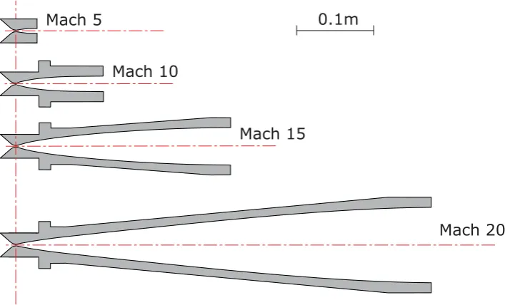
nozzles used in this experiment (figure 1) was designed taking into account the real gas properties, so that the ideal pressure ratios were corrected by numerical calculations of boundary layer and heat exchange. The resulting pressure ratios are slightly different from the corresponding ideal ratios, and are reported in table 1. All the nozzles have the same converging section and throat (diameter=2mm), whilst the diverging section depends on the design Mach number, the relevant output diameters are also reported in table 1.

Mach Number p0/pj output diameter [mm]

5 270.3 6.3

10 6.667×103 24.0

15 4.762×104 71.4

20 1.786×105 121.9

Table 1: Pressure ratios at matched conditions for different Mach numbers

Mach 5

Mach 10

Mach 15

Mach 20

0.1m

Figure 1:The set of nozzles used in this experiment (longitudinal sections)

stagnation pressures are obtained by means of a piston system at the higher Mach numbers and an injector at the lower Mach numbers.

2.2 VACUUMVESSEL

The jets under study are created inside a modular vacuum vessel, with a maximum length of 5m and a diameter of 0.5m. The vacuum is obtained through two vacuum pumps, a lobe pump and a vane pump in cascade configuration, these two devices are capable to lower the internal pressure down to 0.5 – 1 Pa. All parts in the vessel are designed according to the correct principles of vacuum technology [8]. The vessel diameter is much larger than the jets diameter, so the lateral walls effects are negligible and the jets can be considered as free jets until they hit the vessel’s end. The required ambient pressure inside the vessel is obtained by means of a valves system which sets the desired ambient density (at pressures in the range 1.5 to 100 Pa) using a gas in general different from the jet gas. Pressures inside the vessel are monitored by means of two 0.25% accuracy transducers, ranging from 0.01 to 10 Pa and from 0.1 to 100 Pa. The full version of the vessel (figure 2) is composed of three cylindrical sections (2,3,4) plus a head and a tail section (1 and 5). The head segment has a port for the connection of an electron gun, an optical window for a camera and service ports for vacuum pump, ambient gas inlet and electrical connections. Also one of the intermediate sections is provided with similar ports. The modularity of the apparatus involves the considerable advantage of fitting the total volume and length depending on the needs of the individual tests: a larger size is needed to monitor the development of high Mach number jets, because of their larger diameter, in such a way as to follow the jet evolution over a large number of diameters. The sample results presented in this work are obtained by means of a 3-sections setup made of sections 1,2 and 5, where the useful internal vessel length is 2.46 m.

2.3 FASTPISTONSYSTEM

piston/nozzles fitting

aux ports head ports

primary pumps fitting

camera window

nozzle

electron gun head

jet axis

section 5 section 4 section 3 section 2 section 1

Figure 2:Vacuum vessel and experiment setup drawn in full configuration. Top panel: top view. Bottom panel: longitudinal section. The camera window, depending on optical port size and lens in use, is the actual test region.

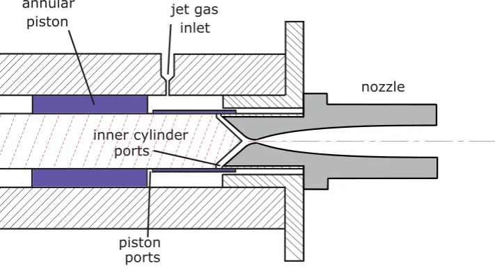
reaches this position, the two sets of ports match each other and the compressed gas flows into the nozzle. The piston is moved by compressed air, it is normally held by an electromagnet and the starting time can be programmed on an electronic timer. The proper use of the piston requires well defined procedures for timing and loading of the jet gas, they are described in the following section. Load pressures are measured by means of 1% accuracy transducers. A separate transducer is available to check stagnation pressures: when needed it can be assembled in place of the nozzle. The resulting repeatability of the jets at each piston run is very good. Of course, the valves require a finite time to pass from the closed to the open condition; therefore the jet mass flow Q has an increasing and a decreasing phase. At the end of compression run, owing to the valves opening, the outflow increases to a maximum value, which is in the order of the mass flow of the same nozzle under steady conditions, then it diminishes as the residual gas contained in the piston is used up. Figure 4 shows a typical gas injection curve.

jet gas inlet

piston ports

nozzle

inner cylinder ports annular

piston

0.00 0.02 0.04 0.06 0.08 0

1 2 3 4 5 6 7

Time [s] Q [kg/s x10-5_]

Figure 4:Jet gas injection: an example of mass flow vs time for an Helium jet at Mach 10

2.4 JET GAS INJECTOR

At the lowest Mach number considered here, the pressure ratio is so low that the piston system cannot afford it, because of leakages and frictional effects. The nominal pressure ratio for Mach 5 is about 270: this means that, for example, a typical ambient pressure in the vessel of 10 Pa, equal to the jet pressure pjunder matched conditions, would require a stagnation pressurep0of 2700 Pa, too low to reach after a

compression run. To reach values ofp0in this range we replace the piston with a direct injection system

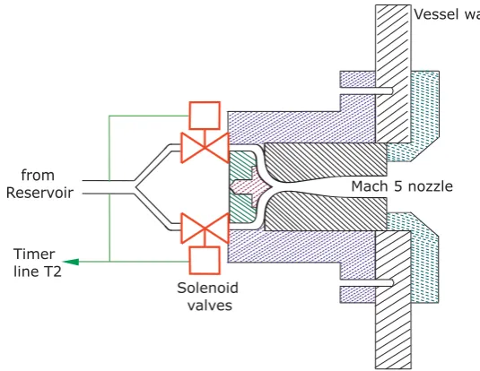
which drives the required low pressure gas into the relevant nozzle. This device receives the jet gas by a set of fast solenoid valves, controlled by an electronic timer. The input pressure is set by extra devices, described in the procedures section. Figure 5 shows a simple sketch of the system, which is usable also with the Mach 10 nozzle.

Vessel wall

Mach 5 nozzle

Solenoid valves from

Reservoir

Timer line T2

Figure 5:Longitudinal section of the injection system for Mach 5

2.5 VISUALIZATIONS AND MEASUREMENT DEVICES

to two turbomolecular pumps. The electron sheet intercepts the jet under test, so that the absorption of light by a population of gas molecules raises their energy level to a brief excited state. As they decay from this excited state, they emit fluorescent light [10]. This fluorescent light generates a plane fluorescent section of the flow and images of the fluorescent zone can be acquired by different kinds of cameras, including intensifiers, depending on the experiment to be performed. The sample results shown in the last section are acquired by a fast CMOS camera (Phantom V5.1) which captures 512x512 or 768x768 monochromatic images at frame rates of 2000 to 5000fps. The camera and the electron gun can be mounted on several ports and optical windows, in the present setup they are mounted on the head section (see figure 2). Besides visualizations, gas densities and structure velocities can be measured by image processing. In particular, the values of the gas density along an image can be obtained by the well known relation between light intensity and gas density [11, 12], taking account carefully of the gas species involved in the measurement. Measurements of velocities can be obtained by standard correlation techniques [13], applied to the typical macroscopic structures appearing in the jet morphology, such as the head bow shock, secondary moving shocks or expansions and mixing layers instabilities.

3 CALIBRATION AND MEASUREMENT TECHNIQUES

In each run at a given Mach number, a pair of gases is selected for jet and ambient. The available gases are helium, argon, xenon and air, only the first three ones are used for the jet since the nozzles are designed for monoatomic gases. The required ambient inside the vessel is obtained by means of a valve injection system which sets the desired ambient density (at pressure in the 1.5 to 20 Pa range) by using a gas in general different from the jet gas.

Cylinder -Piston

System Vacuum Vessel

Jet Gas Bottle

Ambient Gas Bottle

Vacuum Pump Control System

Δt2 Δt1

Pa

Pa tp

air vent Valve

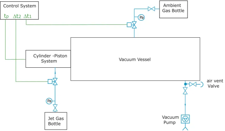
Figure 6:General diagram of the system controls and connections

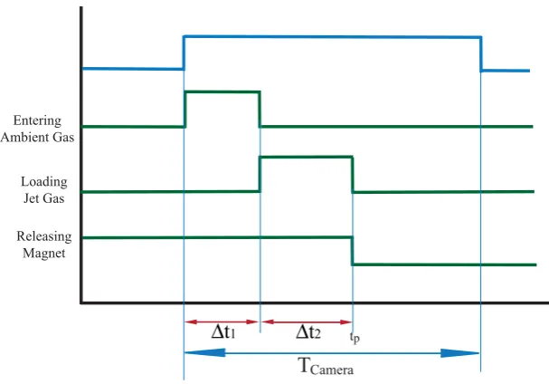
In the general (standard) procedure two solenoid valves must be controlled; one is connected to the vacuum vessel (ambient gas valve) and another one to the fast piston system (jet gas valve), as shown in figure 6. They are operated in sequence, after the adjustment of the time intervalsΔt1 and Δt2in

the electronic timer: Δt1 is the opening time of the first valve which lets ambient gas enter the vessel

and Δt2 is the opening time for loading jet gas in the piston system, immediately after them a third

timer stagetP acts and piston moves (magnet releases), until the compressed jet gas is injected to the

nozzle. The electron gun is turned on before starting the sequence, and the camera stays always on recording mode, and is stopped by a manual post-trigger, retrieving the movie in camera RAM after the experiment. The relevant timing diagram is shown in figure 7.

Entering Ambient Gas

Loading Jet Gas

Releasing Magnet

tp

T

Δ

t

Δ

t

Figure 7: Time diagram of valve system, fast piston system and camera

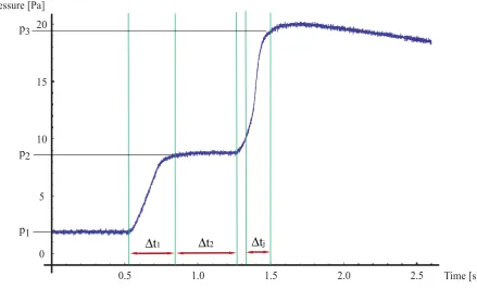
Obviously, the curve doesn’t start from zero, since the vessel is not ideal, and there is always residual air due to unavoidable small leakages. When the first timer stage acts, the first solenoid valve is opened for an intervalΔt1and during this time ambient gas enters the vessel, so the pressure goes up fromp1

(residual air) top2=pa, then during the jet gas loading phase in the cylinder (Δt2), ambient gas reaches

a steady state∗, and just afterΔt2, the magnet releases the piston and, after a fast compression lasting

a measurable time, the jet gas escapes through the nozzle. The jet travels through the vacuum vessel in the subsequent time intervalΔtj, also calledjet lifetime. It can be shown that the duration of the jets

in this experiment is well longer than their physical time scale, defined as the sound crossing time on a jet radius [13], so the jets may be considered nearly steady. However, on the time scale of the operating procedure their lifetime appears always much shorter than the gas loading timesΔt1andΔt2.Δtj can

be estimated directly by the pressure curve as in figure 8, but the final value is safely measured from the movie, since the camera has a very good temporal resolution, working at frame rates in the order of thousands per second. The jet flow leads rapidly the pressure to the maximum valuep3 and finally, at

the end of the experiment, the pressure begin to decrease again because of vacuum pumps.

By pressure diagram, a complete calibration of the system can be stated. About the ambient pressure, it is almost immediate to find calibration charts in the form

pa=F(pas,Δt1) (2)

wherepas (ambient supply pressure) is the pressure fed by the ambient gas bottle. About the jet, the calibration of timeΔt2and piston supply pressureps, in order to obtain a matched jet having the desired properties, is much more complicated as shown in what follows. In the throat of a de Laval nozzle, gas flow is choked, so the equation for the jet mass flow rate can be written in the ideal case by means of standard gas dynamics relations:

˙

m=Acρ0c0

2

γ+ 1 1

2γγ−+11

(3) whereAc is cross-sectional area of the throat whilst ρ0 and c0 are stagnation density and speed of

sound. This formula can be rewritten in terms of stagnation pressure and temperature by means of the ideal gas lawp=ρRjT:

˙

m=Acp0

γ RjT0

1

2 2

γ+ 1 1

2γγ+1−1

. (4)

0.5 1.0 1.5 2.0 2.5 Time [s] 0 5 10 15 20 Pressure [Pa]

Δ

t

p

p

p

Δ

t

Δ

t

Figure 8:Pressure diagram inside the vacuum vessel during a sample run

At the end of the experiment, the jet gas is completely mixed with the ambient gas and it can be assumed that the mixture has the room temperatureTa, because the mass of the ambient gas is much greater

than the one of the jet and because of the fast effect of heat radiation from the vessel walls. Thus the pressure increase due to the jetΔp=p3−p2shown in fig. 8 can be related to the density increaseΔρ

inside the vessel volumeV and to the jet mass flow:

Δp

RjTa = Δρ=

m V =

Δt_j

˙

m

Vdt (5)

Now by replacing (4) in (5) and rearrange the formula it is found:

Δp=AcTa V

Δtj p0

Rjγ

T0

1

2 2

γ+ 1 1

2γγ+1−1

dt (6)

Here the crucial parametersp0 and T0 are not independent since they are due to the compression in

the piston. For a fast ideal isentropic compression they can be related to the supply pressureps and

temperatureTs=Ta, i.e.pandT of the gas loaded from the bottle into the piston,

T0=Ts

p0

ps

γ−1 γ

. (7)

The combination of (5) and (6) leads to:

Δp= AcTa V

Δtj p0

ps

p0

γ−1 2γ _Rjγ

Ta

1

2 2

γ+ 1 1

2γγ+1−1

dt (8)

This formula shows how the final increase in vessel pressureΔpand the jet lifetimeΔtj are related to

the pressurepsof gas initially loaded into the piston and to the stagnation pressurep0 at the end of the

compression.Δp,Δtjandpscan be measured directly, so the formula can be used to expressp0, which

in turn depends on the gas loading timeΔt2, and finally leads to calibration charts of the kind

whereΔtjdoesn’t appear because it is not an independent parameter, actually the jet lifetime for a given

nozzle properly working depends on the quantity of gas available, which is automatically set by selecting ps,Δt2. Up to now, the derivation of the calibration charts was based on ideal conditions, as a further

step accurate calibration charts must then be obtained including corrections for non ideal effects like small heat losses, dependence on the piston driving pressure, frictional effects and progressive opening of the piston valves, so that they take the form

p0=G(ps,Δt2, pp, k) (10)

whereppis the piston driving pressure andkis a set of coefficients related to the laboratory conditions.

Finally, the values of p0 and T0 yield pressure, temperature and density at nozzle exit, so that the

calibration charts can be used to set the desired properties.

For example, first step to get an hypersonic jet is to find a good pressure ratio for a given de Laval nozzle (table 1). Then, after having set piston driving pressure and supply pressures, changingΔt1

andΔt2gives different pressures for ambient and jet respectively. Typically, for a given nozzle, a set of

experiments is performed changing the parametersΔt1,Δt2whilstpas,psandppare kept constants, in

general they are set afresh when a new nozzle is assembled on the system. Furthermore, in a set of experimentsΔt2can be adjusted to obtain well matched jets or even slightly unmatched jets, having a

jet-to-ambient pressure ratiopj/pain an approximated range 0.7 to 1.3, since the boundary layer inside

the nozzles has stabilizing effects against the pressure unmatching [14]; this gives rise to interesting flow morphologies, appearing as perturbations of a properly matched jet (for slightly unmatched jets it is also possible to calculate corrections to the nominal Mach number). Bringing the pressure ratio outside of this range leads instead to the formation of strong shocks and expansions close to the nozzle exit, i.e. to definitely over- or underexpanded jets. In general, these jets are greatly affected by turbulence, so that the mixing with the surrounding ambient becomes faster than in matched jets; when this phenomenon takes place, it can be observed in the camera window.

The research project is divided in four parts; for each part a nozzle, i.e. a nominal Mach number is chosen, then density ratio is varied by selecting different gases and/or adjusting the pressure ratio. In what follows, first part is Mach 20, second Mach 15, third Mach 10, and fourth is Mach 5. The experimental procedure for each part is different from the other ones as explained below.

3.1 MACH20 PROCEDURES

The de Laval nozzle for Mach 20 has a large diameter, so that it is necessary to put the vessel in a long configuration in order to observe jets extending for a sufficient number of initial diameters. According to table 1, matched pressure ratiop0/pj is close to 180000, so for a typical test at ambient pressure pa up to 10 Pa, stagnation pressure should grow up to about 18 bar, what may create safety problems in our system. The solution is to decrease ambient pressure to the minimum value (about 1.5 Pa), but as mentioned, vacuum vessel is not ideal and at low pressures residual air becomes predominant. To overcome this problem, vessel is filled by ambient gas up to more than 20 Pa, then a timer let the vacuum pumps work for a given time, in such a way as when vessel pressure reaches again the minimum level, the residual gas can be considered almost pure ambient gas. Timer stageΔt2 must be set in advance

in order to obtain the desired jet, and after this point the general procedure described above can be followed until the experiment is completed.

3.2 MACH15 PROCEDURES

According to table 1, the matched pressure ratiop0/pjfor Mach 15 is about 48000, well affordable by the

system in standard configuration. In this case the standard procedure described above can be followed as it stands.

3.3 MACH10 PROCEDURES

For Mach 10 the calibration and test procedures are more complicated. The main issue is the matched pressure ratiop0/pj, which in this case is about 6700. One way to obtain this pressure ratio is increase

pressures, another system has been designed. As shown in Figure 9, a small reservoir has been added to the jet gas pipe to keep inside it some amount of gas; its pressure is a bit more that atmospheric pressure. Once this reservoir is full, the valve of jet gas bottle is closed and by adjusting a precision valve connected to the vacuum pumps, the pressure of jet gas in the reservoir is reduced to the desirable one (in the order of 0.4 bar). Again, the desired pressure ratio is obtained by presettingΔt1andΔt2.

Cylinder -Piston

System Vacuum Vessel

Ambient Gas Bottle

Vacuum Pump

Pa

Jet Gas Bottle Reservoir

Pa

Pa

Control System

Δt2Δt1

tp

air vent Valve

High Precision Valve

Figure 9: Sketch of modified system for Mach 10

3.4 MACH5 PROCEDURES

The test procedures for this part are necessarily different because of the new device used instead of the piston. The setup for this case is shown in Figure 10. At first the reservoir is emptied by opening

air vent Valve Injection

System Vacuum Vessel

Jet Gas Bottle

Ambient Gas Bottle

Vacuum Pump Control System

Δt2 Δt1

Reservoir

Pa

Pa

Pa

High Precision Valves

Figure 10:Sketch of modified system for Mach 5

Δt1sets the ambient as before, but the stageΔt2controls directly the injection, i.e. the gas flows through

the injector for the timeΔt2, then the flow is interrupted. Jet duration is thus directly set by the opening

time of the valves connected to the injector. In this case the third timer stage is not used. At the time of writing this report, the first tests of this injector are in progress.

4 RESULTS

In this section, we present some sample results obtained by the present experimental system.

Figure 11 shows the head of a xenon jet traveling in an argon ambient, it is a matched jet obtained by setting a stagnation/ambient pressure ratiop0/pa = 5.17·104±10% and an ambient pressure pa =

10.5±0.1Pa. These parameters lead to a nearly matched jet having at the nozzle exit a Mach number M = 15.1and a density ratioη= 77, thus the jet is highlyoverdensein comparison with the surrounding ambient. The jet structure visible in figure 11 may be interpreted as follows [2]: the jet head is made of a bow shock, traveling left to right, clearly visible in figure, followed by a terminal shock much smaller than the bow shock, and in this case very close to it, so that it cannot be resolved in the image. On the right of the bow-terminal shock structure, only the unperturbed ambient gas is visible; on the left of this structure, the jet core is clearly visible, it is made of xenon traveling at a velocityvg which can be estimated about

(560±20)m/s. This velocity is larger than the one of the shock structurevh= (210±50)m/s, measured

by correlation techniques, so that the jet gas, after being decelerated by the terminal shock, is deflected sideways and form a small backward flowing region behind the bow shock, the so-calledcocoon, which then mixes with the ambient gas. Since the velocity of the head structure is known, two images in succession can be superimposed after shifting the second one by the displacement of the structure under study. Then, this procedure can be repeated, so that a reconstruction of a part of the jet structure can be done by superimposing parts of adjacent frames, obtaining an image larger than what the camera window allows. This method is used for all the figures in this section; of course, it has a physical meaning only if the changes in structure properties are slow in comparison with the interframe time.

Figure 11: Head region of a heavy jet, Xenon in Argon atM = 15.1, density ratioη = 77. The vertical size of the image is 340mm = 9.5 nozzle radii.

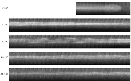
The images presented here come from a movie made of 150 frames taken at 4300 frames per s, an outline of the movie converted in reconstructed parts of the jet is presented in figure 12. Frame 15 to 30, as in figure 11, show the morphology of this jet as a free flow, i.e. practically not perturbed by the walls effects. After image 30, the jet head impacts the vessel end, so that a strong backflow is generated and the flow inside the vessel becomes a jet surrounded by a coaxial stream flowing backward (this is not a naturally backward flow like the cocoon). Under these conditions, the interface between the two flows becomes unstable, so that strong waves appear, they move forward at high velocitiesvi > vh and are

particularly visible in the frames 61 to 90.

Figure 13 shows a helium jet traveling in a xenon ambient, it is a slightly unmatched jet obtained by setting a stagnation/ambient pressure ratiop0/pa = 3.88·104±20% and an ambient pressure pa =

15-30

121-150 91-120 61-90 31-60

Figure 12: Sequence of reconstructed images for the heavy jet Xe in Ar atM = 15.1,η = 77obtained as superpositions of scaled correlated frames from the original movie. The numbers on the left refer to the frame positions in the movie.

unstable interface between jet gas and ambient gas. Here also the velocities are very different from the overdense jet case, actually the core gas velocityvgcan be estimated about(3200±300)m/s, whilst the measured value of the head structure isvh = (350±50)m/s, so the ratiovg/vh is much higher in this case.

Figure 13: Head region of a light jet, helium in xenon atM = 13.4, density ratioη = 0.9. The vertical size of the image is the same as in fig. 11, 340mm = 9.5 nozzle radii.

Figure 14 shows a helium jet traveling in a xenon ambient, it is a nearly matched jet obtained by setting a stagnation/ambient pressure ratiop0/pa = 6.61·103±10% and an ambient pressurepa= 5.1±0.1Pa.

These parameters lead to a jet having at the nozzle exit a Mach numberM = 9.9and a density ratio η= 0.8, thus the jet is again underdense, with a density ratio close to the one of the jet in figure 13, but a slower Mach number. This figure has the same scale of figures 11 and 13. The lower Mach number leads to a new change in the jet morphology. Here the general morphology of the terminal/bow shock structure appears similar to the one in figure 13, but the profile of the bow shock is blunter than in the previous case, as it can be expected for a lower Mach number. Furthermore, the size of the cocoon, if compared with the size of the jet core, is even larger than in previous case, again this is an expected effect of the lower Mach number [13, 15]. In this case the core gas velocityvgcan be estimated about

Figure 14:Head region of a light jet, helium in xenon atM = 9.9, density ratioη= 0.8. The vertical size of the image is the same as in fig. 13, 340mm = 28.3 nozzle radii in this case.

5 CONCLUSIONS

The whole facility is reliable in the different configurations and usable in a wide range of Mach Numbers. The use of matched or quasi-matched de Laval nozzles allows to have rather well known boundary conditions of the jets. The calibration procedures developed for the different Mach Numbers are also reliable, so that the set of experiments may be further carried on following the ones yet conducted, where the whole set of experimental conditions is well and clearly defined. Thanks to the geometry of the devices for the jet generation, even the repeatability of each experiment is very good.

The distance of observation, as referred to the initial jet diameter, is far larger than any of the available experiment and is in the range of stellar jets, while it is not the only purpose of these facilities, as shown e.g. in [6]. Although real stellar jets are not generated in this way, the development of the jets and of the observed instabilities in form of ”knots” are not related to boundary conditions but are part of the jet development itself. Both overdense and underdense jets may be simulated in a wide range of density ratios and this has allowed to have an insight in the change both in jet and cocoon structures, and also in the instabilities that appear on streams interfaces. The fact that the jet structure is persistent even after the impact on the vessel end, although is not part of the stellar jets effort of simulations, is interesting as it is a new piece of knowledge.

About the results, it has been shown that many of the facets of stellar jets may be simulated in a pure fluid dynamic experiment, without the need of electromagnetic fields, what is an important issued in astrophysics [13]. Although the quality of the images is not so good as desirable, due to the camera limits, they may be elaborated to get enough data, while the use of a camera with higher performances is the most urgent further development of the experimental setup.

REFERENCES

[1] Ferrari A.: Modeling extragalactic jets, Annual Rev. Astron. & Astrophys.36539, 1998

[2] Gouveia Dal Pino E.M.: Astrophysical jets and outflows, Advances in Space Research35908–924, 2005

[3] Bellan P.M., Livio M., Kato Y., Lebedev S.V., Ray T.P., Ferrari A., Hartigan P., Frank A., Foster J.M., Nicolaï P.: Astrophysical jets: Observations, numerical simulations, and laboratory experiments, Phys. Plasmas164, 2009

[4] Belan M., Tordella D., De Ponte S.: A system of fast acceleration of a mass of gas for the laboratory simulation of stellar jets, 19th ICIASF, Cleveland, August 27-30, 2001

[5] Belan M., De Ponte S., Massaglia S., Tordella D.: Experiments and numerical simulations on the mid-term evolution of hypersonic jets, Astrophys Space Sci 293 (1-2): 225-232, 2004

[6] Belan M., De Ponte S., Tordella D.: Determination of density and concentration from fluorescent images of a gas flow, Exp. Fluids45501511, 2008

[7] Belan M., De Ponte S., Tordella D.: Highly underexpanded jets in the presence of a density jump between an ambient gas and a jet, Physical Review E82026303, 2010

[9] Bakish R., Wiley J. & Sons: Introduction to Electron Beam Technology, NY, 1962

[10] Brown L.O., Miller N.: α-Ray induced luminescence of gases, Trans. Faraday Soc. 53: 748, 1957 [11] Muntz E.P.: The electron beam fluorescence technique, AGARDograph 132, 1968

[12] Bütefisch K.A, Vennemann D.: The electron-beam technique in hypersonic rarefied gas dynamics, Prog Aer Sci 15: 217-255, 1974

[13] Tordella D., Belan M., Massaglia S., De Ponte S., Mignone A., Bodenschatz E, Ferrari A.: Astro-physical jets: insight into long term hydrodynamics, New J of Physics 13, 043011, 2011

[14] Huzel D.K., Huang D.H: Design of liquid propellant rocket engines, NASA report SP-125, 1967 [15] Massaglia S., Bodo G., Ferrari A.: Dynamical and radiative properties of astrophysical supersonic