When are Identification Protocols with Sparse
Challenges Safe? The Case of the Coskun and Herley
Attack
Hassan Jameel Asghar and Mohamed Ali Kaafar
Data61, CSIRO, Sydney, Australia {hassan.asghar, dali.kaafar}@data61.csiro.au
December 24, 2015
Abstract
Cryptographic identification protocols enable a prover to prove its identity to a verifier. A subclass of such protocols are shared-secret challenge-response identifi-cation protocols in which the prover and the verifier share the same secret and the prover has to respond to a series of challenges from the verifier. When the prover is a human, as opposed to a machine, such protocols are called human identifica-tion protocols. To make human identificaidentifica-tion protocols usable, protocol designers have proposed different techniques in the literature. One such technique is to make the challengessparse, in the sense that only a subset of the shared secret is used to compute the response to each challenge. Coskun and Herley demonstrated a generic attack on shared-secret challenge-response type identification protocols which use sparse challenges. They showed that if the subset of the secret used is too small, an eavesdropper can learn the secret after observing a small number of challenge-response pairs. Unfortunately, from their results, it is not possible to find the safe number of challenge-response pairs a sparse-challenge protocol can be used for, without actually implementing the attack on the protocol and weeding out unsafe parameter sizes. Such a task can be time-consuming and computation-ally infeasible if the subset of the secret used is not small enough. In this work, we show an analytical estimate of the number of challenge-response pairs required by an eavesdropper to find the secret through the Coskun and Herley attack. Against this number, we also give an analytical estimate of the time complexity of the attack. Our results will help protocol designers to choose safe parameter sizes for identification protocols that employ sparse challenges.
1
Introduction
An identification protocol is a cryptographic protocol through which a proverP verifies its identity to a verifier V [1]. A protocol is referred to as a challenge-response type identification protocol whenP andV share the same secret, andP responds to a series of challenges fromV.1 Usually, the response is computed from a publicly known function
f of the secret sand the challenge cso that the verifier can check if the responses are correct at its end. When the proverPis a human, the identification protocol is generally known as a human identification protocol. The holy grail of protocol designers in the realm of human identification protocols is to devise a function f that is simple enough
for a human to mentally compute yet requires the eavesdropper to observe a sizeable number of challenge-response pairs to reconstruct the secret.
Another way to make the identification protocol practical for humans is to reduce the size of the challengecsuch that the functionf is applicable to only a small fractionu
of the shared secrets. We refer to such protocols assparse-challengeprotocols. Given a generic sparse-challenge protocol, Coskun and Herley [2] showed an attack that exploits the observation that whenuis small,candidatesof the secret that are close to the secret
s(in terms of a distance metric) yield similar responses toswhenf is applied on them. In a nutshell, their attack samples a large enough subset S0 of the set of all possible secretsS such that with high probability there is at least one element (candidate) inS0
that is a distance ξfrom the target secrets. The attacker can apply the functionf on each of the candidates in S0 and the observed challenges to weed out those candidates whose responses are further away from the observed responses.2 For more details, see [2]. We call this attack, the CH attack in short.
The CH attack demonstrates that with small values ofu, say≤10, sparse-challenge identification protocols are not secure in the sense that the attack is computationally feasible with a small number of observed challenge-response pairsm. Furthermore, the complexity of the attack can be decreased by observing more challenge-response pairs. However, Coskun and Herley’s work leaves open the following question: Suppose a time complexity of 2λ is considered infeasible for someλ,3what value of missafe enough in
the sense that if the eavesdropper observes≤mchallenge-response pairs, the CH attack has complexity at least 2λ? Indeed, this question is important for protocol designers who wish to use higher values ofu(perhaps for authentication of pervasive devices if higher values ofuare considered infeasible for humans). While it is possible to implement the CH attack to check its feasibility on a given protocol when the sizes of the protocol parameters are small, for larger sizes and largemthis may be impractical.
In this paper, we describe an analytical estimate for m that is safe against the CH attack. Against this safe value of m we also describe a simpler estimate of the work factor (WF) of the CH attack, compared to the analytically difficult expression obtained by Coskun and Herley in [2], to determine the complexity of the attack. Our results can help protocol designers in setting sizes of the protocol parameter, such that the protocol can safely be used for mrounds (challenge-response pairs) against the CH attack with complexity≈2λ, whereλcan be chosen according to what is considered infeasible.4
2
Preliminaries
LetCdenote the challenge space,Rthe response space andSthe secret space, all three being finite sets. A member c ∈ C is called a challenge, r ∈ R a response and s∈ S
a secret. We let log2|S| = η. Then a secret s ∈ S is represented as a binary string of η bits. A fraction u < η are used to compute a function f : C×S →R.5 Given
two stringsx1 andx2 of equal length, the Hamming distance, denotedd(x1, x2), is the
number of positions at whichx1 andx2differ. For two secretss1, s2∈S, it follows that
0 ≤d(s1, s2)≤η. If d(s1, s2) = iwe say that s1 is a distance-i neighbour of s2 (and
vice versa). We let s0 ∈ S denote the target secret. Any other element s∈ S− {s0}
is then called a candidate for the secret, or simply a candidate. Given a sequence of challenges (c1, . . . , cm), let Γ(s) denote the string of responsesf(c1, s)|| · · · ||f(cm, s), for some s ∈ S. Where there is no ambiguity, we shall denote Γ(s) simply by Γ. The
2The notion of distance shall be made exact later. 3For instance,λ= 80.
4Aftermrounds, the secret can be renewed.
5The verifier in fact samples a randomc∈Cin each round such that a randomuout ofηbits ofs
response stream of the target secrets0 shall be denoted by Γ0. For integersxandy, we
use the convention that the binomial coefficient xy= 0, wheneverx < y. The following two well-known results will be used later.
Theorem 1 (Central Limit Theorem [3, §8.3, p. 434]). Let X1, X2, . . . , Xm be a
se-quence of i.i.d. random variables each having mean µand variance σ2. Then
P Pm
i=1Xi−mµ
σ√m ≤a
→Φ(a)asm→ ∞,
where Φ(·) denotes the cumulative distribution function of the standard normal distri-bution.
Theorem 2 (Hoeffding’s Inequality [4, p. 217]). Let X1, X2, . . . , Xm be independent
bounded random variables such that Xi falls in the interval [ai, bi] with probability one.
Then for anyt >0,
P "m
X
i=0
Xi− m
X
i=0
E[Xi]≥t #
≤exp
− 2t
2
Pm
i=0(bi−ai)2
, and P " m X i=0
Xi− m
X
i=0
E[Xi]≤ −t #
≤exp
− 2t
2
Pm
i=0(bi−ai)2
.
The following result will come handy
Proposition 1. For allx∈R, x(1−x)≤1 4.
Let X denote a Bernoulli random variable with distribution P(x), for x∈X. We shall denote the probability thatX = 1 asP(X = 1) =P(1) =p. LetP andQbe two
probability distributions, then the Kullback-Leibler divergence ofQfromP is
D(P||Q) =X x∈X
P(x) log2P(x)
Q(x),
which for Bernoulli distributionsP andQis,
D(P ||Q) =plog2p
q+ (1−p) log2
1−p
1−q,
where we use the convention that log20a = 0 for anya≥0. The following useful bound bears resemblance to a result from [5, p. 2].
Theorem 3. Let P and Q be two Bernoulli distributions with 0 < q < p < 1. Then D(P||Q)≤1
θ(p−q)
2, whereθ= minx{x(1−x)} for allx∈[q, p].
Proof.
D(P ||Q) =plog2
p
q + (1−p) log2
1−p
1−q
=plog2
p e e
q+ (1−p) log2
1−p e
e
1−q
=plnp
q+ (1−p) ln
1−p
1−q
=p Z p
q 1
xdx−(1−p) Z p
q 1 1−xdx
=
Z p
q
p−x x(1−x)
dx ≤ 1 θ Z p q
(p−x)dx=1
θ(p−q)
Finally we shall utilize Sanov’s theorem.
Theorem 4 (Sanov’s Theorem [6, §11.4, p. 362]). Let X1, X2, . . . , Xm be i.i.d. with
distribution Q and let Qm =Q
iQ(xi). Let E be a set of distributions such that E is
the closure of its interior, then
Qm(E∩ Pm) =Qm(E)→2−mD(P∗||Q) asm→ ∞,
where Pm is the set of all empirical probability distributions with denominator m and
P∗ is the distribution inE that minimizes D(P||Q)forP∈E.
Corollary 1. LetX1, X2, . . . , Xmbe i.i.d. Bernoulli random variables with distribution
Q. Then,
P "m
X
i=1
Xi≥mα
#
=Qm(E),
for0< α <1, whereE is the set of distributions
E=
P
X
x∈{0,1}
P(x)≥α=P(1)≥α
.
Moreover, theP∗ that minimizes D(P ||Q)isPα given byPα(1) =α.
Proof. The proof of the first part is in [6, §11.4, p. 361]. For the second part, the distributionP∗ that minimizesD(P ||Q) forP∈E is given by [6,§11.5, p. 364]
P∗(x) = q
x(1−q)(1−x)exp(κx)
qexp(κx) + 1−q ,
whereκis chosen such thatP∗(1) =α. SettingP∗(1) =αin the above, we get
exp(κ) = α 1−α
1−q q ,
which after substitution yieldsP∗(x) =αx(1−α)(1−x)=Pα(x).
3
Analysis of the Coskun and Herley Attack
We shall begin this section by giving an overview of the Coskun and Herley (CH) attack. After that we shall derive an estimate of a safem, i.e., the allowed number of challenge-response pairs. Finally we shall give an estimate of the work factor of the CH attack against this safem.
3.1
Overview of the CH Attack
We assume an eavesdropper, i.e., a passive adversary, observing challenge-response pairs exchanged betweenP andV who share a target secrets0∈S. Each challenge-response
pair is assumed to come from oneround of the protocol. Our discussion in this section is from the adversary’s viewpoint. Assume we have observed mchallenge-response pairs, and we wish to retrieve the target secrets0. Fix aξ∈ {1, . . . , η−u}. The CH attack is
Attack: The CH Attack
1 Sample a random subset S0 ofS with 2η/ ηξcandidates. 2 foreach candidate s0 in S0 do
3 Initialize a list with s0. 4 fori= 0,1, . . . , ξ−1do
5 Computed(Γ0,Γ) of each distance-1 neighbour sof each element in list.
6 Retain τ candidates in the list that maximised(Γ0,Γ).
7 if d(Γ0,Γ) =m for any candidate secret in the list then
8 Output the candidate and halt.
The parameterτ is used to reduce the complexity of the attack. Coskun and Herley use τ = 10 (which we shall also adopt for our simulations). Note that if ξ = 0 the complexity of the attack is equivalent to brute-force, and we therefore use ξ >0. The reason for choosing 2η/ η
ξ
candidates is to expect at least one distance-ξneighbour ofs0
to be present. Increasing this to a factor 2η+q/ ηξ, whereq≥1 increases the probability of this event [2]. However, q = 0 corresponds to least computational overhead, and hence we use this in this paper. A glance at the attack reveals that a large ξ reduces the complexity of the attack (since 2η/ η
ξ
decreases as ξ increases), while a small ξ
increases the probability of finding the secret (as there are less number of iterations, i.e., step 4, and therefore less chance of error). For large values ofξ, we therefore need a larger value of m to successfully find the secret. Next, we show how to estimate a “safe”m, denoted ˆm, for a givenξ. By safe we mean that if the adversary observes less than ˆmchallenge-response pairs, the success probability of the CH attack is low. After estimating an expression for ˆm, we shall derive a simpler estimate for the work factor (WF) of the CH attack obtained by Coskun and Herley, first for a generalm and then in particular for a given value of ˆm.
3.2
Estimating a Safe
m
For reasons of usability, the size of the response space R in a human identification protocol is in general small. Thus, there is a high probability|R|−1that a candidate s
has the same response as s0 on a given challenge. Over m challenges this probability
reduces to|R|−m. Thus a fraction η
|R|m of the candidates, i.e., elements ofS, agree with
the response stream Γ0of lengthm. This imposes aninformation theoreticbound onm
beyond which we expect only the target secrets0 to satisfy the target response stream
Γ0. This bound, denoted mit, is given as logη
2|R|. Thus the attacker has to observe at leastmitchallenge-response pairs to obtain the unique secret, independent of any attack. Our estimation of a safem, i.e., ˆm, for the CH attack shall be meaningful only when it is higher thanmit.
Lets∈S be such thatd(s0, s) =i. Given a uniformly randomc∈C, letpi denote the probability thatf(c, s) =f(c, s0). Then
pi=ai+ (1−ai) 1
|R|
=ai
1− 1 |R|
+ 1
|R|, (1)
where
ai
def
= η−i
u
η u
. (2)
Theorem 5. Let i < j < η, then pi ≥pj, with equality if and only if η−iand η−j
are both less thanu.
Proof. When bothη−iandη−jare less than 0, then by convention η−ui
= η−uj
= 0, and hencepi=pj= |R1|. When η−i≥uandη−j < u, thenai ≥1, whereasaj = 0, from which it follows that pi > pj. We are left with the case when η −i > u and
η−j≥u. Sincei < j < η, we haveη−i > η−j which allows us to write
η−i u
= (η−i) (η−i−u)·
(η−i−1) (η−i−u−1)· · ·
(η−j+ 1) (η−j+ 1−u)·
η−j u
>1·1· · ·1· η−j
u
=
η−j
u
.
This implies thatai> aj and consequentlypi> pj.
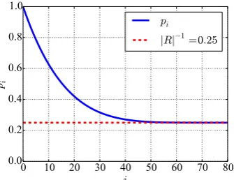
Figure1shows the value ofpiasiranges from 0 toη, forη= 80,u= 5 and|R|= 4. Notice how after around i= η2 thepi’s are closer to|R|−1 = 0.25. Now, as before let
0 10 20 30 40 50 60 70 80
i
0.0 0.2 0.4 0.6 0.8 1.0
p
ip
i|
R
|−1=0
.
25
Figure 1: The graph ofpi asiranges from 0 toη, forη= 80,u= 5 and|R|= 4.
s∈S be such thatd(s, s0) =i. Then the probability that the response stream ofs, i.e.,
Γ, is a distanceγ from Γ0 is given by [2]
P[d(Γ0,Γ) =γ|d(s0, s) =i] =b(γ, m, pi), (3)
whereb(γ, m, pi) is the probability mass function of the binomial distribution given by
b(γ, m, pi) =
m
γ
pγi(1−pi)m−γ. (4)
Letd(s0, s) =ξ, for somes∈S. We shall denote such ansbysξ. Givensξ, letsξ−1and
sξ+1 denote two neighbours ofsξ such that d(s0, sξ−1) =ξ−1 andd(s0, sξ+1) =ξ+ 1.
We are first interested in finding an estimate for m, the number of samples (challenge-response pairs) required to distinguish between Γ(sξ−1) = Γξ−1 and Γ(sξ+1) = Γξ+1.
Such a value ofmensures that with high probability distance-(ξ−1) candidates will be retained in the CH attack as opposed to distance-(ξ+ 1), which in turn will help the attack to move iteratively closer to the target secrets0 [2]. If mis such that it is hard
to distinguish between the response streams Γξ−1and Γξ+1then the CH attack will not
of the CH attack. We will therefore obtain an expression for a safem, i.e., ˆm, through this step.
To do this, first define the Bernoulli random variables
X =
(
1 with probability pξ−1
0 otherwise
and,
Y =
(
1 with probability pξ+1
0 otherwise .
Intuitively,X denotes the indicator random variable which is 1 whensξ−1has the same
response as s0. Likewise for Y. Further define the random variable Z =X−Y. The
expected value ofZ is given by
E[Z]def= µ=E[X]−E[Y] =pξ−1−pξ+1 def
= , (5)
and the variance (assumingX andY to be independent) is given by
Var[Z]def= σ2= (1)2Var[X] + (−1)2Var[Y] =pξ−1(1−pξ−1) +pξ+1(1−pξ+1). (6)
Note that according to Theorem 5, = pξ−1−pξ+1 >0. This is depicted pictorially
below.
pξ+1 pξ pξ−1 p0= 1
Givenmi.i.d. random variablesZiof typeZ, we are then interested in the probability
P "m
X
i=0
Zi≤0
#
, (7)
which estimates the probability that in m challenges the response stream of sξ−1 is
at least as close to s0 as that of sξ+1. In essence, the probability in Eq. 7 is the
error probability that given the stream Γξ+1, adistinguisher erroneously decides that it
belongs to sξ−1. Being asked to give a binary decision, we can assume that the error
probability of the distinguisher is less than or equal to 12. We are interested in finding a bound on the number of samplesm such that the error probability is close to 12. This implies that the distinguisher will not be able to differentiate between the two response streams Γξ−1 and Γξ+1, and hence with high probability CH attack will fail to output
the target secrets0.
Now, we can write Eq.7 as
P "m
X
i=0
Zi≤0
#
=P
"m X
i=0
Zi−mµ≤ −mµ
#
=P Pm
i=0Zi−mµ
σ√m ≤ − mµ σ√m
=P Pm
i=0Zi−mµ
σ√m ≤ − √
mµ σ
→Φ
−
√ mµ σ
where we have applied Theorem1 in the last step. Fix an error probabilityδ. Then we want
Φ
−
√ mµ σ
≥δ
⇒ −√m≥ σ µΦ
−1(δ)
⇒m≤ σ
µΦ −1(δ)
2
, (9)
where the change in the inequality sign follows since Φ−1(δ)≤0 forδ≤ 1
2. Note that we
could also use a concentration inequality, such as Hoeffding’s inequality (Theorem2), to obtain
P "m
X
i=0
Zi≤0
#
=P " m
X
i=0
Zi− m
X
i=0
E[Zi]≤ −m #
≤exp
− 2
2
Pm
i=04
= exp
−
2m
2
,
where we have used the fact thatai=−1,bi= 1 andE[Zi] =µ=. But this serves as
an upper bound on the tail of the error probability, and will only give us a lower bound
m≥ −2
2ln(δ), (10)
for the minimum number of samples required for a fixed upper bound on the tail of the error probability δ. This is contrary to our purpose, which is to find a “safe” upper bound onmsuch that the error probability is close to 12.
We define our bound on mfrom Eq.9 by fixingδ= 0.495, which gives us
ˆ
mdef=
σ µΦ
−1(0.495)
2 ≈ σ
2
µ2(−0.0125) 2≈ σ
2
µ20.00016 =
0.00016σ2
2 , (11)
where values ofandσ2 are as given in Eq.5and Eq.6, respectively.
3.2.1 Empirical Evaluation
Since this ˆmcorresponds to a probability of error close to 1
2, the CH attack should be
unsuccessful with (observed)m≤mˆ. Since we rely on some simplifying assumptions to obtain this estimate, such as the independence ofX andY, and normal approximation through the central limit theorem, it is worthwhile to verify this estimate empirically. To do this, we ran thesubroutine of the CH attack which uses a distance-ξneighbour of
s0on a simulated identification protocol (as was done by Coskun and Herley [2]). More
specifically, we choose a randoms ∈S− {s0} such that d(s, s0) = ξ, and run steps 2
to 8 of Attack 1. This relieves us of having to weed through 2η/ η ξ
candidates, which would require considerable time. Thus, a randoms ∈S− {s0} was chosen each time
such thatd(s, s0) =ξ. Each new random challenge was simulated by randomly sampling
ubits out ofη of the (initially randomly chosen) target secrets0 (thus simulating the
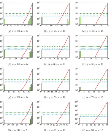
was created which had the u-bit string as the key, and the response as the value. For different sets of values of η andu, we ran the CH attack subroutine 25 times once per each value ofξ, starting at 1, until the estimate ˆm was greater than 10,000 challenge-response pairs. The results are shown in Figure 2. The information theoretic lower boundmit= logη
2|R| is also indicated in the plots. We can see from the plots that with higher values ofη and u, i.e., Figures 2e, 2f, 2h, 2i, 2k and 2l, the success probability is 0 against ˆmobtained through Eq. 11. For Figure2l, we extend thecut-off value of
ˆ
mto 60,000 challenge-response pairs. As is shown, the success rate of the CH attacks is still 0. We remark that while we have chosen δ= 0.495, any value ofδclose to 0.5 should suffice. For instance, our simulations also found δ = 0.490 to be a safe choice. Of course,δ = 0.490 gives a higher value of ˆm versus δ= 0.495 for a fixed value of ξ. Lowering δfurther, say to 0.400, is not recommended as a safe choice. Figure 3 shows why.
3.3
Estimating the Work Factor
In this section we obtain a simple analytical estimate for the work factor (WF) of the CH attack. Note that we are interested in finding a value ofλsuch that 2λ≈WF. Therefore, an estimate that is off by a couple of powers of 2 is sufficient for our purposes. Whenever we shall plot WF, it will be in log2-scale. The work factor of the CH attack is given by [2, p. 434]6
WF = 1η ξ
2η+τ ηξ
η
X
i=0
η i
m
X
j=mpξ
m j
pji(1−pi)m−j
, (12)
where againτ is a threshold set at 10 by Coskun and Herley, and mpξ is the boundary chosen such that candidates with response streams that are a distance less than mpξ from the target secret’s response stream are discarded [2]. Define
WF1=
2η η ξ
, (13)
which we call the brute-force term as in [2]. Let
αi
def
= m
X
j=mpξ
m j
pji(1−pi)m−j, (14)
and define the right hand term
WF2=
τ ηξ
η ξ
η
X
i=0
η i
αi. (15)
Given a value of ˆm for a fixed value of ξ calculated through Eq. 11, one can directly measure WF through Eq. 12. However, there are two problems with this approach. First as ˆm grows larger, the αi’s are computationally expensive to compute. Indeed, Coskun and Herley only showed an estimate of the work factor for u= 5 [2, p. 437]. Secondly, not much insight is possible from this rather crude expression of WF. We therefore explore this expression further.
6To be precise, the work factor should be multiplied bym(the number of observed challenge-response
0 5 10 15 20 25 30 35 40 100
101
102
103
104
(a)η= 50, u= 5
0 5 10 15 20 25 100
101
102
103
104
(b)η= 50, u= 10
0 5 10 15 20 100
101
102
103
104
(c)η= 50, u= 15
0 10 20 30 40 100
101
102
103
104
(d)η= 60, u= 5
0 5 10 15 20 25 30 100
101
102
103
104
(e)η= 60, u= 10
0 5 10 15 20 25 100
101
102
103
104
(f)η= 60, u= 15
0 10 20 30 40 50 100
101
102
103
104
(g)η= 70, u= 5
0 5 10 15 20 25 30 35 100
101
102
103
104
(h)η= 70, u= 10
0 5 10 15 20 25 100
101
102
103
104
(i)η= 70, u= 15
0 10 20 30 40 50 60 100
101
102
103
104
(j)η= 80, u= 5
0 5 10 15 20 25 30 35 40 100
101
102
103
104
(k)η= 80, u= 10
0 5 10 15 20 25 30 35 100
101
102
103
104
105
(l)η= 80, u= 15
Figure 2: The values of ˆm according to Eq.11 and the success percentage of the CH attack against increasing values of ξ (x-axis) and . |R| is fixed at 4. The y-axis is log-scaled. Legend: mˆ; mit; — success percentage;××100% success boundary; ++50% success boundary.
First, we find an estimate for the αi’s. Note that in essence,αi is the proportion of the binomial ηi
retained. Define Bernoulli random variables
Xi=
(
1 with probability pi
0 otherwise . (16)
0 5 10 15 20
ξ
100
101
102
103
104
105
106
ˆ
m
m
it 100%50% success %
Figure 3: The values of ˆm according to Eq.11 and the success percentage of the CH attack against increasing values ofξwhenη= 80,u= 15 andδ= 0.400 in Eq.11. Note high success rate of the CH attack.
we have
P
m
X
j=1
Xi,j≥mpξ
→2−
mD(Pξ||Pi) asm→ ∞
From this we may estimate theαi≈2−mD(Pξ||Pi)wheni≥ξandαi≈1−2−mD(Pξ||Pi) when i < ξ (see for instance Figure 4). However, as indicated by Figure 1, for larger
mpξ mpξ−1
mpξ+1
Figure 4: The portions of the binomials retained in the CH attack where: portion retained; portion discarded. Note thatαξ = 0.5,αi >0.5 fori < ξ and αi <0.5 for
i > ξ.
values ofξ, sayξ > η2, the difference in probabilities is very small for the neighbours of
sξ, and therefore our bound ofαi, which is based on large deviations assumption, will err. One way to compensate for this is to instead use the normal approximation of the
αi’s as Φ(−
√
mµXi
σXi ) for the nearby neighbours of sξ whenξ > η
2 in a manner similar to
Section3.2, whereµXi =pi andσ 2
Xi =pi(1−pi). A less messier way is to upper bound
theαi’s by 0.5 fori > ξand lower bound by 0.5 fori < ξ, indicating that these sums are not expected to exceed these limits (see Figure4). This gives us the following estimate
αi≈
max{1−2−mD(Pξ||Pi),0.5} ifi < ξ
0.5 ifi=ξ
min{0.5,2−mD(Pξ||Pi)} ifi > ξ
With this estimate of the αi’s we denote the corresponding estimate of WF2 byWFˆ 2.
Figure5shows the actual work factor WF2against our estimateWFˆ 2. Note thatWFˆ 2is
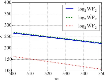
expected to be a better estimate than simply approximating all theαi’s by the standard normal estimate (not just the neighbours of αξ), since the standard normal estimate is poor for larger deviations. To show this, we illustrate WF2 against WFˆ 2 and the
standard normal estimate, denotedWF˜ 2, in Figure6 for η = 800. Notice howWF˜ 2 is
many orders of magnitude off. To get high precision values, we implementedWF˜ 2using
thempmathPython library [7] with a precision of 200 decimal places.
0 50 100 150 200 0
20 40 60 80 100
(a)η= 80, u= 15, ξ= 1
0 50 100 150 200 0
20 40 60 80 100
(b)η= 80, u= 15, ξ= 10
0 50 100 150 200 0
20 40 60 80 100
(c)η= 80, u= 15, ξ= 60
Figure 5: Actual work factor WF2 versus the estimatedWFˆ 2 whenη= 80,u= 15 and
ξ∈ {1,10,60}againstmin the range [1,200]. Legend: log2WF2; log2WFˆ 2.
500 510 520 530 540 550
m
100 150 200 250 300 350 400
λ
log
2WF
2log
2WF
ˆ
2log
2WF
˜
2Figure 6: Work factor WF2 and its estimates forη= 800,u= 25 andξ= 10. Theλin
they-axis indicates power of 2. Notice howWF˜ 2 is off the mark.
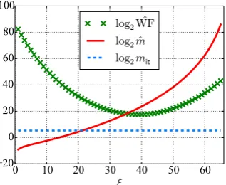
We can now see the evolution of the estimate of the work factor ˆWF against ˆm(using
δ= 0.495 in Eq.11) as shown in Figure7, which is obtained by replacing WF2 byWFˆ 2
in Eq.12. The figure indicates that the computational complexity of the CH attack is minimized atξ≈ η
2. We now show that this is true in general for suitably large values
ofu. In the process, we also obtain a simplified expression of ˆWF. Fix a 0< β <1 such thatu=βn. We want to show that for a suitably largeβ (say 101), theαi’s are at least 0.5 for alli∈ {1, . . . , ξ, . . . , η−u}. From the definition of theαi’s in Eq.17it is obvious that fori≤ξ, αi≥0.5. For i > ξ, showing that αi≥0.5 is the same as showing that 2−mDˆ (Pξ||Pi) ≥2−1 ⇒ −mDˆ (P
0 10 20 30 40 50 60
ξ
20 0 20 40 60 80 100log
2WF
ˆ
log
2m
ˆ
log
2m
itFigure 7: The total work factorWF forˆ η= 80 andu= 15 against ˆmforδ= 0.495.
Eq.11, we get
ˆ
mD(Pξ ||Pi) =
σ2z2
2 D(Pξ ||Pi)
≤ σ
2z2
(pξ−1−pξ+1)2
1
θ(pξ−pi)
2
=σ
2z2
θ
(pξ−pi)2 (pξ−1−pξ+1)2
≤z
2
2θ
(pξ−pi)2 (pξ−1−pξ)2
,
where we have used the fact thatσ2≤ 1
2 (by applying Proposition1on Eq.6). Now for
i >
(pξ−pi)2≤
pξ−
1 |R| 2 = η−ξ u η u
1− 1 |R|
!2 ,
and
(pξ−1−pξ)2=
η−ξ+1
u
− η−uξ
η u
1− 1 |R|
!2
=
η−ξ+ 1 η−ξ+ 1−u−1
η−ξ u η u
1− 1 |R|
!2
=
u η−ξ+ 1−u
2 η−ξ
u η u
1− 1 |R|
!2 .
Substituting these values and simplifying we obtain
ˆ
mD(Pξ ||Pi)≤
z2
2θ
η−ξ+ 1−u u
2 .
Now, substitutingu=βn, we get
η−ξ+ 1−u u
2
= 1
β2
1−ξ η +
1
η −β 2
≤ 1
β2(1−β)
Also, for all i∈ {1, . . . , η−u}, thepi that minimizespi(1−pi) corresponds toi= 1. Now,
p1=
η−1
u η u
1− 1 |R|
+ 1
|R|
= η−u
η
1− 1 |R|
+ 1
|R|
= (1−β)
1− 1 |R|
+ 1
|R| (substitutingu=βη)
= 1−β
1− 1 |R|
.
Letθi correspond to theθ in Theorem 3 with the associated interval [pξ, pi]. If we let
θ= mini{θi}, then
θ=p1(1−p1)
=
1−β
1− 1 |R|
β
1− 1 |R|
=β2 1
β −
1− 1
|R| 1−
1
|R|
> β2 1
β −1
|R| −1
|R| (since|R| −1>0)
⇒ 1 θ <
1
β2
β
1−β |R| |R| −1
≤ 2 β2
β
1−β (since|R| ≥2).
Substituting these results into the expression for ˆmD(Pξ||Pi) we finally obtain
ˆ
mD(Pξ ||Pi)≤
z2
2 2
β2
β
1−β
1
β2(1−β) 2
= z
2
β4β(1−β)
≤1
4
z2 β4,
where the last inequality follows from Proposition1. The above is less than or equal to
1 ifβ ≥ q
|z|
2. Since according to Eq.11, we chose|z| ≈0.0125, it follows thatβ ≥0.08
suffices as a choice.7 From this it implies that 2−mDˆ (Pξ||Pi) ≥0.5. Therefore WFˆ 2 for
ˆ
mis at least
ˆ WF2=
τ ηξ η ξ η X i=0 η i
αi ≥
τ ηξ η ξ 1 22 η= τ ηξ η ξ 2
η−1. (18)
Note that as the binomial sum has a maximum value of 2η, the above work factor is close to the maximum, since for ˆm
ˆ WF2≤
τ ηξ
η ξ
2
η.
The above expression has a minimum at aroundξ= η2.8 This is true since ηξ=O(ηξ) for ξ≤ η
2 and
η ξ
=O(ηη−ξ) for ξ > η
2, and the terms
ξ
ηξ and
ξ
ηη−ξ have a minimum
when ξ = η2. Substituting WF2 with the value of WFˆ 2 obtained through Eq. 18 in
Eq.12, we see that the total work factor WF is dominated by WF2when m= ˆm(and
u≥βη), since
WF≈ (2 +ητ ηξ)
ξ
2
η−1≈τ ηξ
η ξ
2
η−1.
We summarise our findings in the following heuristic theorem.
Theorem 6. Let pi be as defined by Eq.1fori∈ {0,1, . . . , η}. Further, letmˆ = σz
2 where
2= (pξ−1−pξ+1)2 andσ2=pξ−1(1−pξ−1) +pξ+1(1−pξ+1),
andz= Φ−1(δ) for someδ∈(0,12). Then if u≥βη, where β=
q |z|
2, the work factor
of the Coskun and Herley attack is
WF≈ τ ηξη
ξ
2
η−1,
which is minimum whenξ=η2, for1≥ξ≥η−uandu≤ η2. Ifu > η2 the minimum is achieved at ξ=η−u.
We reiterate that we are interested in finding λsuch that 2λ ≈WF, and hence an estimate that is far from the true value by a few of powers of 2 is sufficient.
4
Case Study: Setting Parameter Sizes for
Identifi-cation Protocols
Suppose we a proverP and a verifierV share a secretswhich is a set ofkindexes out ofn. All indexes are from the set{1, . . . , n},nbeing a positive integer. We denote this set of indexes by [n]. Consider the following identification protocol betweenP andV:
Protocol:An Identification Protocol
1 V sends a challengectoP which is a random subset of indexes from [n] of cardinalityl,l < n, such that each element is associated with a randomweight
from Z4.
2 P initializesr1←0.
3 foreach index iin cdo 4 if i∈sthen
5 P updatesr1←r1+w, wherewis the weight associated withi. 6 P computesr2←r1mod 4.
7 if r2∈ {0,1}then
8 P returnsr←0 as its response. 9 else if r2∈ {2,3}then
10 P returnsr←1 as its response. 11 V acceptsP if the responseris correct.
The protocol above is known as the Foxtail protocol with window [8]. In an actual protocol, the above process is repeated a number of times per authentication session such that the probability of randomly guessing the response (without knowing anything
about the secret!) is low. But for our purposes we ignore this detail, and assume that there is one round per authentication session. The term window alludes to the
l-element challenge presented to the prover. Since a fraction of the secretsis expected to be present in each challenge, CH attack can be applied to the protocol to find the secret. The question arises, with a given set of values of protocol parameters (l, k, n), how many rounds can the above protocol be used for, i.e., the value of m, so that the CH attack has complexity of about 2λfor a fixed λ? We first estimate uas follows
u= E[|s∩c|]
k η=
E[|s∩c|] k log2
n k
=lk
n
1
klog2 n
k
= l
nlog2 n
k
, (19)
where lkn is the expected value of the hypergeometric distribution. If we choosekandn
to be such thatη = log2 nk
≈80 (e.g., n= 180 and k= 18), and choosel = 40, then we getu≈0.22×80≈18 bits. We can now choose a δ to obtain a value of ˆm using Theorem 6 which in turn gives us a value forλ, i.e., log2WF. If a work factor of 225 is considered infeasible, i.e., λ= 25, then withδ = 0.495, we can use the protocol for
m≤993 ≈1,000 (which corresponds to ξ= 25). Choosing δ= 0.490 allows us to use the protocol form≤3,972≈4,000 rounds (again corresponding toξ= 25).
5
The CH Attack is not always Optimal
Consider the variant of the above protocol in which the weights are from Z2 and the
response is simply r ← r1mod 2. Then we can use Gaussian elimination to find the
secretsafternobservations, by constructing then×nbinary matrixH whose rows are constructed from m=n observed challenges and using the n-element response vector
r obtained from the responses. On the other hand, the CH attack requires a much larger number of observationsmto be feasible, providedlandnare not too small. For instance, if (l, k, n) = (40,18,180), as above, with m ≈ 262 > n, the work factor of the CH attack is ≈258. Gaussian elimination on the other hand is a polynomial time
algorithm that would yield the secret afterm≈n= 180 observations.
Of course, for Gaussian elimination to yield a unique solution we require the nrows (or equivalently, columns) of H to be linearly independent. We show here that this is likely to happen with high probability. Note that the total number of possible challenges in this protocol are
|C|= l
X
i=0
n
i
,
which can be arrived at by observing that there are ni
possible binary vectors with Hamming weighti. From this we could use a counting argument to get the number of possible combinations of n linearly independent vectors, by iteratively discarding any linearly dependent choices for the vector i given i−1 linearly independent vectors. However, this is not straightforward, as the linear combination of any two vectors inC
might not be a vector inC (e.g., two vectors with Hamming weightl which differ in at least one position). Asymptotic results, however, suggest that iflis large enough we are likely to construct a full rankn×nmatrixH after observing m > nchallenges, where the differencem−nis bounded from below by a constant. To be precise, we reword the corollary from [9] as a theorem using our notation.
Theorem 7. Let m > n. Ifl >lnn+ω(1)andm−n≥ω(1), then almost every set of muniformly random vectors from C havenlinearly independent vectors.9
9Recall thatf=ω(g) means that f(n)
As an example, for the case under consideration, i.e.,n= 180 andl = 40, a simple Python script using theSage library10 returned a full rank n×n matrixH, each row of which was randomly sampled fromC, at a success rate of 0.2969 (over 10,000 repe-titions). In contrast,l= 2 returned 0 such incidences. The fact that the success rate is high for reasonably large values oflis not surprising. For instance, a necessary condition for the matrix H to be linearly independent is to have no zero columns. Observe that the probability of an element from a vectorc∈Cbeing zero is given by
1 2·
l n+ 1·
1− l n
= 1− l
2n,
which follows since either the element could be absent from thel chosen elements, or it could be present but with weight 0. Let Bi be the probability that the ith column is
not a zero column vector, then
P(Bi) = 1−
1− l
2n n
.
LetAbe the event that the matrixH has no zero column vectors, then
P(A) =
n
\
i=1
P(Bi)
≥
n
X
i=1
P(Bi) !
−n+ 1
= 1−n
1− l
2n n
which is close to 1 for sufficiently largel andn(the inequality above is the application of Benferroni’s inequality [3, §7, p. 426]). For instance, when n = 180, l = 15 yields
P(A)>0.91.
6
Related Work
Baign`eres, Junod and Vaudenay [10] show a more general result which estimates the number of samples required by an optimal distinguish between two probability distribu-tions (not necessarily Bernoulli) that are close to each other. Barring constant factors, the estimate from them and the two estimates given in Eq.9and Eq.10all yieldm∼ 1
2, which can be used as arough guide for the number of samples required in our case.
We note that somewhat similar to our estimation ofm, the work in [8,§5] attempts to bound the safe number of rounds against counting based statistical attacks on human identification protocols introduced by Yan et al. [11]. However, the resultant figures for the number of safe rounds against these counting based attacks are erroneous, since they do not treat the associated probability as an error probability, and wrongly calculate the required samples by fixing the one-sided cumulative distribution function of the standard normal distribution at 0.6.
Research on human identification protocols dates back to the work of Matsumoto and Imai in [12]. Juels and Weis [13] noted parallels between humans and resource-constrained devices, that both suffer from low computational and memory capabilities, and proposed a variant of the Hopper and Blum (HB) human identification protocol [14] to be used for identification of such devices. To the best of our knowledge, to date, this
10
is the only human identification protocol whose application as an identification protocol for resource-constrained devices has been extensively studied. It is an interesting area of research to analyze other human identification protocols, such as the sum of kmins protocol [14], for their suitability as identification protocols for resource constrained devices. While some of the human identification protocols in literature are based on ad hoc design [12, 15,16], there are others whose security is based on the hardness of interesting mathematical problems [17,18, 19,20,21]. There are also some theoretical advances in generic attacks on human identification protocols [2,11,8,22]. These results may result in other human identification protocols being proposed for identification of resource-constrained devices.
7
Conclusion
We have shown estimates for the number of sessions that should be allowed before secret renewal in challenge-response type identification protocols, which use a fraction of the secret to respond to a challenge, to be safe against the Coskun and Herley attack. We have also shown how we can estimate the work factor of this attack against the number of allowable sessions in a computationally efficient and protocol independent manner. These estimates are empirically straightforward to obtain without the need to implement the Coskun and Herley attack on a given protocol to check its complexity against different sets of values of protocol parameters. This work can benefit protocol designers to set parameter sizes both in the field of human identification protocols or identification protocol for resource constrained devices in which the use of “sparse” challenges is desirable.
References
[1] Berry Schoenmakers. Lecture Notes Cryptographic Protocols. Version 1.1, http: //www.win.tue.nl/~berry/2WC13/LectureNotes.pdf, 2015.
[2] Baris Coskun and Cormac Herley. Can “Something You Know” Be Saved?. In Tzong-Chen Wu, Chin-Laung Lei, Vincent Rijmen, and Der-Tsai Lee, editors,ISC ’08, pages 421–440. Springer, 2008.
[3] Sheldon M. Ross. A First Course in Probability. Prentice Hall, 4 edition, 2002.
[4] St´ephane Boucheron, G´abor Lugosi, and Olivier Bousquet. Concentration Inequal-ities. InAdvanced Lectures in Machine Learning, pages 208–240. Springer, 2004.
[5] Robert L. Wolpert. Markov, Chebychev and Hoeffding Inequalities. Lecture notes, https://stat.duke.edu/courses/Spring09/sta205/lec/hoef.pdf, 2009.
[6] Thomas M. Cover and Joy A. Thomas. Elements of Information Theory. John WIley and Sons, Hoboken, New Jersey, USA, 2nd edition, 2006.
[7] Fredrik Johansson et al. mpmath: a Python library for arbitrary-precision floating-point arithmetic (version 0.18), December 2013. http://mpmath.org/.
[9] Nathan Linial and Dror Weitz. Random vectors of bounded weight and their linear dependencies. http://dimacs.rutgers.edu/~dror/pubs/rand_mat.pdf, 2000.
[10] T. Baign`eres, P. Junod, and S. Vaudenay. How far can we go beyond linear crypt-analysis? In P.J. Lee, editor,Advances in Cryptology -Asiacrypt’04, volume 3329 ofLecture Notes in Computer Science, pages 432–450. Springer-Verlag, 2004.
[11] Qiang Yan, Jin Han, Yingjiu Li, and Robert H. Deng. On Limitations of De-signing Leakage-Resilient Password Systems: Attacks, Principals and Usability. In
19th Annual Network and Distributed System Security Symposium, NDSS ’12. The Internet Society, 2012.
[12] T. Matsumoto and H. Imai. Human identification through insecure channel. In
EUROCRYPT ’91, pages 409–421. Springer-Verlag, 1991.
[13] Ari Juels and Stephen A. Weis. Authenticating Pervasive Devices with Human Protocols. InProceedings of the 25th Annual International Conference on Advances in Cryptology, CRYPTO ’05, pages 293–308, Berlin, Heidelberg, 2005. Springer-Verlag.
[14] N. J. Hopper and M. Blum. Secure Human Identification Protocols. In ASI-ACRYPT ’01, pages 52–66. Springer-Verlag, 2001.
[15] Daphna Weinshall. Cognitive Authentication Schemes Safe Against Spyware (Short Paper). InIEEE Symposium on Security and Privacy, SP ’06, pages 295–300. IEEE Computer Society, 2006.
[16] M. Lei, Y. Xiao, S. V. Vrbsky, and C.-C. Li. Virtual Password using Random Linear Functions for On-line Services, ATM Machines, and Pervasive Computing.
Computer Communications, 31(18):4367–4375, 2008.
[17] Hassan Jameel Asghar, Josef Pieprzyk, and Huaxiong Wang. A New Human Iden-tification Protocol and Coppersmith’s Baby-step Giant-step Algorithm. In Pro-ceedings of the 8th International Conference on Applied Cryptography and Network Security, ACNS ’10, pages 349–366, Berlin, Heidelberg, 2010. Springer-Verlag.
[18] L. Sobrado and J.-C. Birget. Graphical Passwords. The Rutgers Scholar, 4, 2002.
[19] S. Wiedenbeck, J. Waters, L. Sobrado, and J.-C. Birget. Design and Evaluation of a Shoulder-Surfing Resistant Graphical Password Scheme. In AVI ’06, pages 177–184. ACM, 2006.
[20] S. Li and H.-Y. Shum. Secure Human-Computer Identification (Interface) Systems against Peeping Attacks: SecHCI. IACR’s Cryptology ePrint Archive: Report 2005/268,http://eprint.iacr.org/2005/268, 2005.
[21] Jeremiah Blocki, Manuel Blum, Anupam Datta, and Santosh Vempala. Human Computable Passwords. arXiv preprint arXiv:1404.0024http://arxiv.org/pdf/ 1404.0024.pdf, 2014.