Oscillatory Models for Biological Signal Processing and Pattern
Recognition
Tetiana Aksenova1,*, and Tatyana V. Ryzhkova2
1
Univ. Grenoble Alpes, CEA, LETI, CLINATEC, F-38000 Grenoble, France 2
Plekhanov Russian University of Economics, RU-117997, Moscow, Russia
Abstract. Among biomedical signals, repetitive or quasi-periodic signals are particularly widespread. While the periodic component is still presented these signals are characterized by period variations (fundamental frequency, amplitude, etc.). The lack of synchronization or phase shifts results in variations in similar segments’ durations, nominally identical signals demonstrate a variation at peak retention times, etc. The inverse methods of oscillation theory were proposed recently as a tool to solve the problems of modelling of repetitive signals with phase shift. In the article, the inverse method of oscillation theory is considered as a tool to solve the problems of supervised and non-supervised classification, and filtering of repetitive signals with phase shift. Examples of application are presented.
1 Introduction
Among biomedical signals, repetitive or quasi-periodic signals are particularly widespread. While the periodic component is still presented in these signals they are characterized by period variations (fundamental frequency, amplitude, etc.). More generally, one of the problems of the study of biological signals is the lack of synchronization or phase shifts which results in variations in similar segments’ durations, nominally identical signals demonstrate a variation at peak retention times, etc. Generally, the phase shift cannot be compensated with linear methods and/or efficiently described as an additive noise. In contrast, statistical methods of regression analysis and classification are generally based on the assumption of the presence of additive noise only which describes the distortion in amplitude alone, and are sensitive to disturbances to this assumption. This explains the low prediction ability of traditional methods of applied statistics applied to raw signals with phase shift (e.g. [1]).
Several approaches were proposed to tackle the problem. One of the approaches is the segmentation of signals for subsequent modelling, classification, etc. (e.g. [2,3]). Segmentation is commonly applied to treat quasi-periodic physiologic signals, such as in pulse oximetry and electrocardiograms (the tracing of the cardiac cycle consists in the detection of the P wave, QRS complex, etc.). However, the presence in the recording of artefacts and noise caused by patient movement or electrical interference reduces the accuracy of algorithms based on segmentation [4]. Normalization to the same duration is often used for the data preprocessing. It compensates to some extent the non-stability of the signals in temporal domain. Nevertheless, even after normalization signals
often demonstrate significant variations in peak retention time [5]. Consequently, the distance between nominally identical signals can be large in ordinary Euclidian space [6]. Window Preprocessing (WP) can improve the signal presentation. WP divides the region of observation into windows and counts the statistic of the peaks within each of them [5]. However, if the window boundaries are located in the peak region, the efficiency of WP may be impaired. Various transformations (spectral, wavelet transform, etc. (e.g. [7, 8]) are applied to avoid temporal signal presentation. Last decades, Dynamic Time Warping (DTW) [9] and variants become popular approach for measuring similarity between two temporal sequences, which vary in speed. The sequences are "warped" in the time to measure sequences similarity independent of non-linear variations in the time dimension. Sequences averaging and classification according to DTW were considered [10-13]. Nevertheless, even techniques for DTW faster computing were proposed (e.g. [13, 14]) signal processing task with regard to DTW are still computationally inefficient [13].
By contrast, IMOT based algorithms are sufficiently efficient to be applied in real time [15].
The study began in the 1960s. The self-oscillation model with perturbation was applied to describe processes in astrophysics and in medicine (electrocardiograms and electrokymograms modelling [16]. Statistical-correlation methods was proposed to identify such models from observations [17]. Later, a range of problems of statistical signal processing were considered by authors [6, 18-20].
In the article, the IMOT methods are revised as a tool to solve the problems of statistical signal processing, such as averaging, supervised and non-supervised classification, and filtering out of repetitive signals with phase shift. Examples of application are considered.
2
Methods
2.1. Model description
For the sake of simplicity, let us consider a scalar case. Let us assume that the signal is observed with additive noise, which is a sequence of i.i.d. random variables with zero mean and finite variance 𝑥𝑥�(𝑡𝑡) =𝑥𝑥(𝑡𝑡) +𝜉𝜉(𝑡𝑡), while the signal itself is assumed to be a solution of an ordinary differential equation with perturbation:
+
= −− −− t
dt x d x F dt x d x f dt x d n n n n n n , ,..., ,..., 1 1 1 1
,
(1)where
= ,..., −n1−1
n n n dt x d x f dt x d (2)
describes a self-oscillating system with a stable limit cycle 𝐱𝐱0(𝑡𝑡) =�𝑥𝑥10(𝑡𝑡), … ,𝑥𝑥𝑛𝑛0(𝑡𝑡)�′, 0 <𝑡𝑡 ≤ 𝑇𝑇, in phase
space with co-ordinates 𝑥𝑥1=𝑥𝑥,𝑥𝑥1=𝑑𝑑𝑑𝑑
𝑑𝑑𝑑𝑑, … ,𝑥𝑥1= 𝑑𝑑𝑛𝑛−1𝑑𝑑 𝑑𝑑𝑑𝑑𝑛𝑛−1. Here n is the order of the equation, T is the period of stable oscillations. The perturbation function F(), bounded by a small value, is a random process with a zero mean and a correlation time ∆tcorr that is small in comparison to the period of stable oscillations ∆tcorr << T. The perturbation function F() tends to displace the trajectories of the signal out of the limit trajectory. However, if the perturbation is small enough, the trajectories remain in the neighborhood of the limit cycle if the initial point is located in the neighborhood. As a result, the observed solutions are similar to one another, but they never coincide.
For further applications, the model (1-2) is parameterized using Poincare sections [21] (Fig.1). Let us introduce [22] the local coordinates in the neighborhood of the limit cycle. Let us fix an arbitrary point on the limit cycle P0 as a starting point. The position of any point P on the limit trajectory can be described by its phase 𝜃𝜃, which is a time movement along the limit cycle from a starting point P0 (𝜃𝜃= 0). If function f() is twice continuously differentiable on all arguments, providing the necessary smoothness, at a point P with phase 𝜃𝜃 it is possible to construct a
hyperplane (and only one such hyperplane) that is normal to the limit cycle [22]. We denote M(𝜃𝜃) as the point of intersection with the hyperplane of phase 𝜃𝜃 and set the point of phase zero to M(0)=M0 (𝜃𝜃= 0), as the initial point for the analyzed trajectory. Any trajectory can be described by variables n(𝜃𝜃) and t(𝜃𝜃) (Fig. 1) where n(𝜃𝜃) is a vector of normal deviation defined by M(𝜃𝜃) and its orthogonal projection P(𝜃𝜃) on the limit cycle. The second variable t(𝜃𝜃) is a time movement along the trajectory from the initial point M(0) to the analyzed point M(𝜃𝜃). The limit cycle is defined by n(𝜃𝜃)≡ 0 and t(𝜃𝜃)≡ 𝜃𝜃, where 0 is a vector with all components equal to 0.
Let γ(θ) be the phase deviation, γ(θ)= t(𝜃𝜃)-𝜃𝜃. Then (1) can be rewritten in linear approximation in terms of the normal n(𝜃𝜃) and the phase γ(θ) deviations [22]
) ( ) ( ) ( ) ( ) ( θ θ θ γ θ θ θ θ γ F n F n N n + ⋅ Θ = = + d d
d n . (3)
Here N(θ) and Θ(θ) are functions of the parameters. As a result the trajectory in phase space is presented in linear approximation as a sum of a periodic component presented by the limit cycle x0(θ) and functions of deviations: x(t(θ))=x0(θ) + n(θ), where n(θ) and t(θ)=γ(θ)+θ follow from (3).
Model (1-2) can be compared to the model with additive noise 𝑥𝑥�(t) = 𝑥𝑥0(t) + 𝜉𝜉(t) with periodic expectation x0(t). Both models, describe signals close to periodic ones. However, whereas the model with additive noise explains the distortion in amplitude alone, the model of nonlinear oscillations with perturbations explains the distortion of both the amplitude and phase.
A scalar case is considered in present article. Example of application of IMOT to vector case can be seen in [20].
2.2 Parametersfit from experimental data
After parameterization the model is determined by triplet 𝐌𝐌= (𝐱𝐱0(𝜃𝜃),𝐍𝐍(𝜃𝜃),Θ(𝜃𝜃)). For the following applications, the triplet can be fitted to the experimental data. The limit cycle presents a periodic component of the signal x0(θ), 0<θ ≤ T, with the phase running from 0 to T. Let us refer to the segments of an arbitrary signal trajectory xi(t(θ)), 0<θ ≤ T with phase θ running from 0 to T as cycles. Cycles may have similar but non-identical duration. Let us consider the general population formed by cycles X= {xi(t(θ)), 0<θ ≤ T}. As the mean trajectory converges to the limit cycle x0(θ) in linear approximation if the number of averaged trajectories increases infinitely [17], the limit cycle x0(θ) can be estimated in linear approximation by averaging the observed cycles xi(t(θ)), 0<θ ≤ T in the phase space (Fig. 1)
∑
∑
= = = = k i i k i i i t k tk 1 1
0(~) 1 ( ( )), ~ 1 ( )
~ θ x θ θ θ
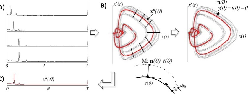
Fig. 1. A) Example of signals with phase shifts stems from chromatographic experiments carried out with High Performance Liquid Chromatography (HPLC) columns. Chromatograms of the same product demonstrate column-to-column, lot-to-lot and day-to-day variations in peak retention time [5]. B) The same set of chromatograms in phase space (x(t), x’(t) projection), the mean trajectory 𝐱𝐱0(𝜃𝜃), normal n(𝜃𝜃) and phase deviations γ(θ)= t(𝜃𝜃)- 𝜃𝜃. C) First coordinate 𝑥𝑥0(𝜃𝜃) of 𝐱𝐱0(𝜃𝜃) represents the mean signal in the temporal domain.
Instead of averaging other statistics can be applied, taking into account that ni(θ) and γi(θ) are characterized by an asymptotically Gaussian distribution in the case of uncorrelated noise F() [17]. As the observed cycles xi(t(θ)) are described as xi(θ+γ(θ))=x0(θ)+ni(θ), 0<θ ≤ T, the first coordinate x0(θ) of mean trajectory in phase space estimates the undisturbed signal in the temporal domain (Fig. 1).
To estimate the functions of the parameters N(θ) and
Θ(θ) the local coordinates (normal and phase deviations) are calculated. Firstly, 𝑡𝑡𝑖𝑖(𝜃𝜃�) are calculated for each i-th
cycle according to the phase. Then,
) ~ ( ~ )) ~ ( ( ) ~
(
θ
θ
0θ
x x
ni = i i −
t , and
γ
i(θ
~)= i(θ
~)−θ
~t ,
T ≤ <θ~
0 are the local coordinates. Interpolation can be used for regular partition in time. The functions of the parameters of (3) may be estimated using e.g. difference equations ) ( ) ( ~ ) ( )) 1 ( ~ ) 1 ( ~ )( 2 / 1 ( ) ( ) ( ~ ) ( )) 1 ( ~ ) 1 ( ~ )( 2 / 1 ( 2 1 θ ε θ θ θ γ θ γ θ ε θ θ θ θ + Θ = − − + + = − − + n n C n
n . (5)
Linear regression techniques can be applied. The training sample set consisted of normal and phase deviations for a given phase across the set of observed cycles [20].
2.3 Signal classification
To consider the problem of signal classification, let us assume that a set of signals/cycles
~
x
i(
t
)
=
x
i(
t
)
+
x
(
t
)
isobserved at discrete times t=0,1,...,𝑇𝑇𝑖𝑖and additive noise is a i.i.d sequence with zero mean and finite variance. Each xi(t), 0 < t≤ 𝑇𝑇𝑖𝑖 is assumed to belong to one of p of
the general populations Xj, 0 ≤ j ≤ p;
Xj={xi(t), 0 < t≤ 𝑇𝑇𝑖𝑖}. The signals from each general population Xj are assumed to be generated by the same ordinary differential equation with perturbation 𝐌𝐌𝑗𝑗=
�𝐱𝐱𝑗𝑗0(𝜃𝜃),𝐍𝐍𝑗𝑗(𝜃𝜃),Θ𝑗𝑗(𝜃𝜃)�.
While the entire triplet may be required (see, for example, [20]), the classification according to the limit cycle only may be applied to solve many problems [6, 18]. Let us firstly consider the problems of the supervised and unsupervised classification of signals with phase shift accordingly.
2.3.1 Supervised classification
The vectors of normal deviation 𝐧𝐧𝑖𝑖(𝜃𝜃) are characterized by an asymptotically Gaussian distribution for any 𝜃𝜃 in the case of uncorrelated noise F(). Thus, the problem of the classification of cycles xi(t(θ))=𝐱𝐱𝑗𝑗0(θ)+ni(θ), 0<θ ≤ T, can be reduced to the separation of a mixture of (asymptotically) normal distributions in the transformed feature space. Let us refer to the space RT of features presenting signal measurements x(ti), at time moments ti = 1,…,T as a standard feature space of dimension T. Then let us consider the space Rn×T, of dimension n×T, of features representing the signal and the derivatives, at time moments t(θi) θi = 1,…,T:
.(𝐱𝐱(𝑡𝑡(𝜃𝜃1)′|𝐱𝐱(𝑡𝑡(𝜃𝜃2))′| … |𝐱𝐱(𝑡𝑡(𝜃𝜃2))′)′,
𝐱𝐱�𝑡𝑡(𝜃𝜃𝑖𝑖)�= (𝑥𝑥1(𝑡𝑡(𝜃𝜃𝑖𝑖)), … ,𝑥𝑥𝑛𝑛(𝑡𝑡(𝜃𝜃𝑖𝑖)))′.
Here the partition of the interval of the signal observation becomes generally irregular in time, i.e.,
𝑡𝑡(𝜃𝜃𝑖𝑖+1)− 𝑡𝑡(𝜃𝜃𝑖𝑖)≠1 and is determined by phase
𝜃𝜃𝑖𝑖 = 1,…,T. Since the vectors of normal deviation
) ( ( ) ( ( )
(
θ
xj tθ
i x0 tθ
in = − have an asymptotically
normal distribution with mathematical expectation close to zero, we obtain p normally distributed classes in the new feature space Ω, with features x(t(θi)), 1 = θ1 <…< θT = T, ∆θ = 1, and Euclidean norm
( )
( )
2 / 1 2 1 0 =∑ ∑
− ≤ ≤ Ωi j n j j t dt x d θ θ
x . (6)
P(θ)
x0(θ)
) (t
x′ n(θ)
γ(θ) = t(θ) − θ ) (t x′ x(t) t T 0
x0(θ)
In the case of supervised classification the number of classes p and the function of belonging for the training set presenting signals from all general populations are known. Limit cycles 𝐱𝐱𝑗𝑗0(𝜃𝜃), 0 < θ ≤ T determine the centers of the classes Xj, and can be calculated for each
of the classes ~x0j(
θ
~), for example, by averaging. Let usremember that function ~x0(
θ
~) (the first component of)
~
(
~
0θ
x
) approximates the mean signal trajectory in the time domain (Fig.1). When the centers of classes are estimated, the classification of new sample is possible using conventional classification method. Using e.g. template matching, minimum distancesΩ
−
=
ip i p
d
(
x
0,
x
)
x
0x
are calculated for the analyzedsignal
x
i(⋅
)
and the centers of classesx
0p(
⋅
)
, p=1,...,m:) , ( min
arg 0 i
p p d
p= x x . (7)
The distance between the two cycles xi(t) and xj(t), 0<t≤T can be approximated by
𝑑𝑑2(𝐱𝐱𝑖𝑖,𝐱𝐱𝑗𝑗) =� 𝛿𝛿2(𝑡𝑡) 𝑇𝑇
𝑑𝑑=0
,
𝛿𝛿(𝑡𝑡) =𝜏𝜏∈(−𝜏𝜏min
𝑚𝑚𝑚𝑚𝑚𝑚,𝜏𝜏𝑚𝑚𝑚𝑚𝑚𝑚)�𝑥𝑥
𝑖𝑖(𝑡𝑡)− 𝑥𝑥𝑗𝑗(𝑡𝑡+𝜏𝜏)�
using an interpolation of the signals. Here τmax is a maximum of the phase deviation.
2.3.2 Unsupervised classification
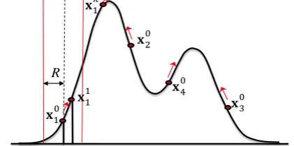
The problem of unsupervised classification of classes with Gaussian distribution is well studied. However, traditional statistical methods, generally, require the calculation of the position of each observation/sample in feature space. This requirement would demand the calculation of the synchronized signal trajectories, estimating t(θi), θi = 1,…,T, for each observed signal which is a problematic issue for unlabeled classes. The presented unsupervised learning algorithm scans a training set to estimate the number of classes and their centers by measuring the pairwise distances between the trajectories in phase space alone. In case of a Gaussian distribution the mathematical expectation corresponds to the maximum of the probability density. The mean trajectory is estimated by an iterative procedure that detects the sample with maximal probability density in its R-neighborhood.
Supposing that the training set T contains only one class trajectories. On the first step the initial estimation of the class center is an arbitrary sample 𝒙𝒙𝟎𝟎. Subset
𝑹𝑹𝟎𝟎 ⊂ 𝑻𝑻 is the R- neighborhood of 𝒙𝒙𝟎𝟎, 𝑹𝑹𝟎𝟎=
{𝒙𝒙 ∈ 𝑻𝑻:‖𝒙𝒙 − 𝒙𝒙𝟎𝟎‖
𝜴𝜴<𝑹𝑹}. The next estimation 𝒙𝒙𝟏𝟏 is the element minimizing the sum of distances between 𝑹𝑹𝟎𝟎 elements: 𝒙𝒙𝟏𝟏=𝒂𝒂𝒂𝒂𝒂𝒂𝒎𝒎𝒎𝒎𝒎𝒎𝒙𝒙∗∑𝒙𝒙∈𝑹𝑹𝟎𝟎‖𝒙𝒙∗− 𝒙𝒙‖𝜴𝜴 . On the next step 𝑹𝑹𝟏𝟏= {𝒙𝒙 ∈ 𝑻𝑻:‖𝒙𝒙 − 𝒙𝒙𝟏𝟏‖𝜴𝜴<𝑹𝑹} is considered, and so on. Due to the symmetry and unimodality, this
procedure converges to the mean value on any choice of the parameter R. However, a larger training set is required for smaller values of R. For the simultaneous search of centers of 𝒑𝒑 classes (𝒑𝒑 is unknown), we assumed that the classes are well separated enough to consider that the maxima of the density of joint distributions are near the centers of the classes. The maxima of the density are the stationary point of the iterative procedure described above. The initial estimates are calculated iteratively (Fig. 2) using the samples out of current set of class center R- neighborhoods. It is possible that from different first estimates the algorithm converges to the same stationary points.
Fig. 2. Iterative procedure for simultaneous search of centers of several classes.
The radii of classes can be estimated by considering the distribution of squares of the pairwise samples distances or squares of the distance of samples to the given center of the class [18, 23].
For classification of new sample conventional classifiers may be employed.
3 Examples of applications
Several real world problems were studied using IMOT approach. Real-time neuronal spikes sorting [15], and the suppression of artefacts of Deep Brain Stimulation (DBS) [24] from neurophysiological recordings [19, 20] are examples of application.
3.1 Unsupervised recognition of neuronal discharge waveforms
Multisite microelectrode recordings are widely used in animal research [25], and in clinical applications [24]. Quick analysis of the biological signals is often required. The extracellular microelectrode recordings register the activity of few neurons located near the microelectrode tip. Observed neurons generate action potentials–spikes. Spike sorting procedure is generally applied to recognize the sequence of spike of individual neurons. Under stationary recording conditions, it can be assumed that a neuron generates spikes with similar dynamics of the membrane potential and can be recognized accordingly.
The detection of the neuronal spikes in the raw signal is the first step of the spike sorting algorithm. The spikes are usually characterized by amplitudes significantly larger than the level of background noise and their occurrence may be detected by threshold crossing. The first and second derivatives of the raw signal were used
𝐱𝐱10
R
𝐱𝐱30 𝐱𝐱11
𝐱𝐱20
to detect the events in [15, 23]. Since the method of computing derivatives has a filtering effect [18], the derivatives are less affected by noise, in particular with
respect to lower frequency components that may be generated by muscles twitch or cardiac artefacts.
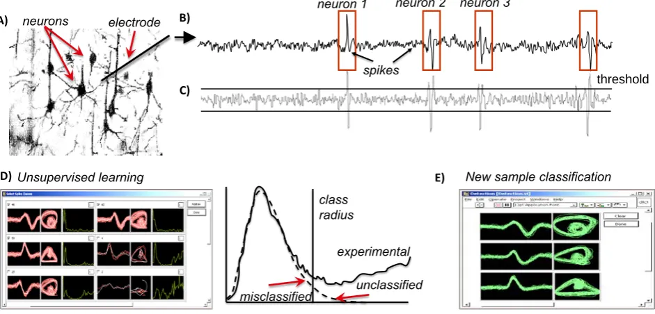
Fig. 3. A) The extracellular microelectrode recordings register the activity of few neurons located near the microelectrode tips. B) Action potential (spikes) of three different neurons registered with one electrode. C) Spike detection from signal derivative. D) Unsupervised learning procedure. The radii of classes is estimated taking into account that the distribution of squares of the distance of spike to the center of the class can be approximated by the χ2 function. The radius of each class is chosen to equalize the misclassified and unclassified errors. E) Classification of newly detected events.
Choosing an appropriate level of confidence, e.g. p=0.99, it is possible to find the threshold for spike detection by considering the distribution of neural signal (Fig 3).
The learning procedure based on iterative
computations is described above. Besides neuronal spikes, detected events may include outliers. The radii of classes were estimated to be used as upper bounds in a decision rule. Due to Gaussian distribution of normal deviation, the distribution of squares of the distance of spike to the center of the class can be efficiently approximated by the χ2 function. The deviation of the experimental distribution from the fitted χ2 provides an estimate of the errors of classification which, in turn, the radii of the classes to be set. In [18], the radius of each class was chosen to equalize the misclassified and unclassified errors (Fig. 3).
Finally, the spike sorting procedure is applied to the data stream [15]. The distances between a newly detected event to all templates are evaluated. In the case the shortest distance is smaller than the specific radius, the event is assigned to that template. For unbalanced classes the class probability may be taking into account using decision function 𝑑𝑑𝑖𝑖(𝐱𝐱) =𝑝𝑝𝑖𝑖𝑝𝑝(𝐱𝐱|𝑋𝑋𝑖𝑖), where 𝑝𝑝𝑖𝑖 is the class 𝑋𝑋𝑖𝑖 probability [23].
In the studies mentioned above, microelectrode distance was large enough to exclude multisite neuronal action potentials observation. Scalar model was consequently applied to each electrode recording.
3.2 Suppression of spurious signals in records of neural activity during Deep Brain Stimulation
High-frequency (100–300 Hz) DBS [24] is a surgical procedure for the treatment of a variety of disabling neurological symptoms, in particular those due to Parkinson’s disease, dystonia, major depression, essential tremor, chronic pain, etc. During the surgical intervention electrodes are implanted in the target zone of the brain to periodically deliver repeated electrical impulses. The optimal localization of DBS electrodes is a crucial problem in the DBS surgery procedure. To locate the most suitable position of the stimulation electrodes, the neuronal activity in the target zone is recorded with microelectrodes during the surgery.
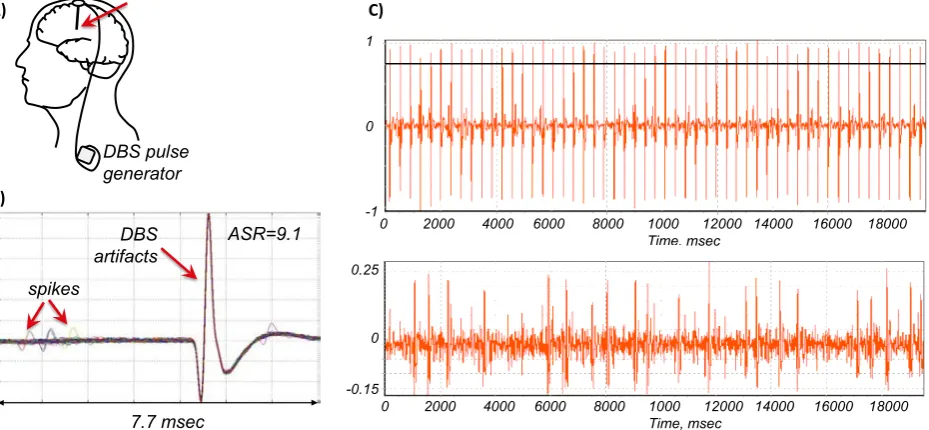
The appropriate signal of neuronal activity during the stimulation, namely the recording of action potentials (spikes), cannot be fully analyzed due to stimulation artifacts. The artifacts of stimulation have huge amplitude in comparison to the meaningful signal. The Artifact-to-Signal Ratio (ASR), the ratio of the amplitudes of the artifacts to the averaged amplitude of the spikes, varies between 3 and 50 (Fig.4). As DBS artifacts and spikes of neuronal activity are highly overlapped in frequency domains, subtraction techniques were developed. However, most of them suffer from an inability to adapt to the nonlinear dynamics of the artifacts, and hence yield large residuals. The conventional methods treat artifacts as signals with additive noise using several templates. Applying these
A
B
C)neurons electrode
A)
D) Unsupervised learning E) New sample classification
misclassified unclassified
experimental class
radius spikes
threshold
neuron 1 neuron 2 neuron 3
methods to the filtering of even moderate artifacts (ASR=5.1) results in signals which still contain residuals that are greater than the meaningful signal [26]. IMOT
approach was applied for stimulation artefacts
subtraction in [19, 20] (Fig.4) allowing explaining the variability in the stimulation artefacts.
Fig. 4. A) Deep Brain Stimulation (DBS): a medical device is surgically implanted to deliver electrical stimulation to targeted areas of the brain through electrodes. The extracellular microelectrode recordings of neuronal activity are registered in parallel to stimulation during DBS surgery. B) Signal of neuronal activity during DBS sliced into stimulation-period windows, ASR=9.1. C) Signal of neuronal activity during DBS before (up) and after (down) stimulation artifact filtering.
Mean artefact is subtracted from signal in phase space in [19]. Periods of stimulation can be easily collected. After averaging in phase space, local coordinates are calculated for each artefact. The normal deviations represent the signal after the filtering. Namely the first coordinates of the normal deviations is the meaningful signal. Interpolation is applied for regular partition in time. This algorithm provides efficient filtering with decreasing of artefact residuals 2-3 times compared to conventional time domain approach. The error rate is sufficiently low (< 3%) for ASR up to 10. Here inter-channel dependences in not taking into account
DBS artifact modelling in deviations is proposed in [20]. Similarly to [19], after the limit cycle is estimated, it is subtracted from the signal according to the synchronization. The resulting functions of normal deviation and phase deviation from the training set are used in order to identify the functions of the parameters for the model in deviations (3). After artifacts are sequentially estimated by numerical integration to be subtracted. The first coordinates of the residual normal deviations is the meaningful signal. In this approach, a key factor is the correct definition of the initial conditions for numerical integration. The initial set-up condition is based on inter-channel adjustment [20]. Hence, the DBS artifacts suppression in deviations can be applied for the multi-channel recordings only. For the data with ASRs equal to 4, and 7, multichannel algorithm gives 1.87% of error in the whole signal, and 20% of error in across the peak window (10% time window). While using the conventional method, 10% of
error in the whole signal is obtained, and the peak neighborhood are completely lost.
4 Perspectives
The studies were primarily directed at problems in biology and medicine. Nevertheless, the proposed methods can be applied in various fields, in particular, for modelling of oscillatory processes in economics. As variation in the described process is phase dependent [17], one of the perspectives may be the optimization of time measurement [27] for efficient observation.
The study was partially supported by NATO HTECH.LG, 972304, INTAS-Ukraine 95-0060, INTAS-OPEN 97-168, INTAS 97-0173, Swiss NSF SCOPES 7IP 62620 grants, and a Medtronic grant to INSERM U318.
References
1. I.V. Tetko, A.E.P. Villa, T.I. Aksenova,
W.L. Zielinski, J. Brouwer, E.R. Collantes, W.J. Welsh, J. Chem. Inf. Comp. Sci., 38, 660-668 (1998)
2. S.A. Vorob'ev, Automat. Rem. Contr., 46, 8(2), 1003-1006 (1986)
3. S.A. Vorob’ev, Theses of Doctor of Science, Tula State University, 328 pp. (2000) [in Russian].
4. G.D. Clifford, F. Azuaje, P.E. McSharry, Advanced Methods and Tools for ECG Data Analysis (Boston, Artech House 2006)
DBS pulse generator electrodes
spikes
7.7 msec
ASR=9.1 DBS
artifacts
0 2000 4000 6000 8000 1000 12000 14000 16000 18000 Time, msec
0 2000 4000 6000 8000 1000 12000 14000 16000 18000 Time, msec
1
0
-1
0.25
0
-0.15
A)
B)
5. W.J. Welsh, W. Lin, S.H. Tersigni, E. Collantes, R. Duta, M. Carey, W.L. Zielinski, J. Brower, J.A. Spencer, T.P. Layloff, Anal. Chem., 68, 3473-3482 (1996)
6. T.I. Aksenova, I.V. Tetko, A.G. Ivakhnenko,
A.E.P. Villa, W.J. Welsh, W.L. Zielinski, Anal. Chem., 71, 2423-2430 (1999)
7. E.R. Collantes, R. Duta, W.J. Welsh, Anal. Chem., 69, 1392–1397 (1997)
8. D. Rafiei, A. Mendelzon, FODO '98 Conference, Kobe, Japan, (1998)
9. D.J. Berndt, J. Clifford, KDD workshop, 10. 16 (1994)
10. F.O. Petitjean, A. Ketterlin, P. Gançarski, Pattern Recognit., 44, 3 (2011)
11. F.O. Petitjean, P. Gançarski, Theor. Comput. Sci., 414, 76–91 (2012)
12. H. Ding, G. Trajcevski, P. Scheuermann, X. Wang, E. Keogh, Proc. VLDB Endow, 1(2), 1542–1552 (2008)
13. A. Mueen, N. Chavoshi, N. Abu-El-Rub,
H. Hamooni, A. Minnich, J. MacCarthy, Knowl. Inf. Syst., 54(1), 237-263 (2018)
14. X. Wang, A. Mueen, H. Ding, G. Trajcevski,
P. Scheuermann, E. Keogh, Data Min. Knowl. Disc., 26(2), 275-309 (2013)
15. Y. Asai, T.I. Aksenova, A.E.P. Villa, LNCS, 3696, 109-114 (2005)
16. L.I. Gudzenko, Statistical method for processing of electrokymograms, Voprisy klinicheskoy biofiziki, Moscow, 33-54 (1966) [in Russian]
17. L.I. Gudzenko, Izv. Vyssh. Uchebn. Zaved., Radiofiz. (Sov. Radioph.), 5, 573-587 (1962) [in Russian]
18. T.I. Aksenova, O.K. Chibirova O.A. Dryga, I.V. Tetko, A.-L. Benabid, A.E.P. Villa, Methods, 30, 178-187 (2003)
19. T.I. Aksenova, D.V. Nowicki, A.-L. Benabid,
Neural Comput., 21, 2648–2666 (2009)
20. D.V. Nowicki, A.-L. Benabid, T.I. Aksenova, International Conference of Numerical Analysis and Applied Mathematics, AIP Conference Proceedings, 936, 382-386 (2007)
21. V.I. Arnold, Méthodes Mathématiques de la
Mécanique Classique, (MIR, Moscow, 1974. Zbl0385, 70001, 1965)
22. A.G. Chertoprud, L.I. Gudzenko, In Kinetics of Simple Models of Oscillating Theory. Moscow, Nauka (1976)
23. A.E.P. Villa, I.V. Tetko, B. Hyland, A. Najem, Proc. Natl. Acad. Sci. USA, 96, 1006–1011 (1999)
24. A.L. Benabid, P. Pollak, C. Gross, D. Hoffmann, A. Benazzouz, D.M. Gao, A. Laurent, M. Gentil, J. Perret, Stereotact. Funct. Neurosurg., 62, 76–84 (1994)
25. O.K., Chibirova, T.I. Aksenova, A.L. Benabid,
S. Chabardes, S. Larouche, J. Rouat, A.E. Villa, Biosystems, 79(1-3), 159-171 (2005)
26. T. Hashimoto, C.M. Elder, J.L. Vitek, J. Neurosci. Methods, 113, 181–186 (2002)