R E S E A R C H
Open Access
Three-Dimensional Position-Based
Adaptive Real-Time Routing Protocol for
wireless sensor networks
Fariborz Entezami
*and Christos Politis
Abstract
Devices for wireless sensor networks (WSN) are limited by power, and thus, routing protocols should be designed with this constraint in mind. WSNs are used in three-dimensional (3D) scenarios such as the surface of sea or lands with different levels of height. This paper presents and evaluates the Three-Dimensional Position-Based Adaptive Real-Time Routing Protocol (3DPBARP) as a novel, real-time, position-based and energy-efficient routing protocol for WSNs. 3DPBARP is a lightweight protocol that reduces the number of nodes which receive the radio frequency (RF) signal using a novel parent forwarding region (PFR) algorithm. 3DPBARP as a Geographical Routing Protocol (GRP) reduces the number of forwarding nodes and thus the traffic and packet collision in the network. A series of performance evaluations through MATLAB and Omnet++ simulations show significant improvements in network performance parameters and total energy consumption over the 3D Position-Based Routing Protocol (3DPBRP) and Directed Flooding Routing Protocol (DFRP).
Keywords: GRP; VNP; 3DPBRP; 3DPBARP; Rainbow; DFRP
1 Introduction
The main duty of a wireless sensor network (WSN) as a distributed computing network is collecting data from a large number of nodes that have the capacity to sense the environment and process data and also communi-cate over a short range. WSN applications collect data from wireless sensors, and an appropriate routing proto-col could help them achieve scalability and improve per-formance. In real-life WSN applications, wireless sensor nodes are deployed in three-dimensional coordinate sys-tem (3D) environments such as mountains or sea surfaces. Most of the position-based routing protocols consider the topology as a two-dimensional scenario. In this paper, deploying wireless sensors in 3D environments has been considered. Data collection protocols can form a planner or tree topology that could be in cluster or mixed data collection form. The Three-Dimensional Position-Based Adaptive Real-Time Routing Protocol (3DPBARP) is one of the many-to-one routing protocols which is based on
*Correspondence: [email protected]
Wireless Multimedia & Networking (WMN) Research Group, Faculty of Science, Engineering and Computing (SEC), Kingston University London, Penrhyn Road, Kingston Upon Thames KT1 2EE, England
the spanning tree method [1, 2]. 3DPBARP establishes at least one data collection tree with a sink as the root node in the topology. All data which are produced by sensors are forwarded to the root node. Each node is responsible not only for sending its own data but also for relaying other’s data, so that they cover more distance to the root node [3, 4]. The Trickle algorithm [5] optimizes the overhead cost and makes the routing protocols more flexible. The control protocol packets are sent based on changes in topology, and if there is no change in topol-ogy, the interval times (duration) between when updates are sent is increased with a resulting decrease in the num-ber of control packets. It also makes routing protocols react quickly and be adaptable to any changes in topology, and if any change in topology is sensed, then the interval time is reset to minimum in order to update the topology very quickly [6, 7]. 3DPBARP enhances greedy forwarding by considering congestion and packet delivery informa-tion when looking for the best path to the destinainforma-tion. 3DPBARP uses a mechanism for choosing a parent that it is based on the spherical distance (SD) value of each neighbour that chooses the best possible parent between existing qualified neighbours. 3DPBARP avoids occurring
a loop in topology by using some mechanism. It also uses the Rainbow mechanism that makes 3DPBARP be able to avoid dead end routes [8]. 3DPBARP uses a new mecha-nism to make it more energy efficient than other existing algorithms. The proposed protocol uses unique restricted parent forwarding regions (PFRs) based on the algorithm that limits the number of nodes that receive the packets. It decreases the radio frequency (RF) range to the minimum to cover the nodes’ parent only, and for this reason, other nodes do not consume energy to receive the signal and retransmit them. Geographical Routing Protocols (GRPs) make all nodes be able to learn more about their location and also the position of neighbours and the sink. GRPs could make decisions with better performance in real-time and dynamic scenarios. GRPs decrease the overhead of the protocols significantly and make them more effi-cient. The disadvantages of GRPs are the cost of additional hardware and also the accuracy of location determina-tion which depends on the mechanism and techniques whether the location of each node is calculated. Some techniques such as radio ranging have less accuracy, and some techniques such as the Global Positioning System (GPS) have more accuracy [9–11].
In this paper, 3DPBARP as a 3D, real-time and geo-graphical routing protocol has been proposed that pro-vides a soft real-time capability for an effective heuristic solution for void node problem or hole problem. The void node problem (VNP) or hole problem is called to a situ-ation when a packet arrives at a node that does not have any neighbour to forward the packet toward the sink. The Rainbow mechanism is used to avoid dead end routes. The proposed protocol also uses a unique restricted PFR-based algorithm that limits the number of nodes that receive the packet.
This paper is organized as follows: Section 2 describes previous works, and Section 3 shows the 3DPBARP design details and system model. Evaluation and results from simulations come in Section 5, and finally, the conclusion is provided in Section 6.
2 Related works
O-CTP [12] is based on investigation of WSN routing protocol behaviour in networks that are affected by inter-ference. O-CTP is a hybrid routing protocol that uses the high packet delivery ratio of opportunistic routing in error-prone networks, and it is also an energy-efficient routing protocol [13].
ICTP [14] uses both long path with good link quality and also short path with bad link quality. It may decrease the reliability, but it improves efficiency to avoid congestion. Li et al. have shown that the energy consumption in ICTP is less than that in the Collection Tree Protocol (CTP) in the same scenarios based on reducing the possibility of congestion.
BCTP [15] is a balanced version of CTP that enables the network to avoid the heavy traffic nodes. It uses average transmission rate as a metric. BCTP has been evaluated by a testbed, and the results show that the load in hot spot drops by 61.9 %. RAP [16] is a real-time GRP which uses the velocity of each packet as a gradient to deliver the packets. Each velocity is calculated based on the distance to the destination and its delivery deadline. The packets with higher velocities can be sent earlier than the pack-ets with lower velocities. However, this protocol does not provide any guarantee in end-to-end real-time delivery. EDF [17] provides a real-time decentralized scheduling that guarantees end-to-end delivery, but it needs a pri-ori defined schedule that is not feasible in most of WSN applications. SPEED [18] is a real-time GRP that uses neighbour information to estimate distance in a routing protocol. SPEED lets each node decide which neighbour would be the next hop forwarding node, and in case there is no suitable node existing in neighbours, the node with the lowest miss ratio is used for forwarding the pack-ets. MMSPEED [19] is an enhanced version of SPEED that focused on reliability levels and multiple timelines. It uses resources with better performance than SPEED. RTLD [17] is a real-time routing protocol with load bal-ancing based on link quality, packet delay and remaining power in the next-hop neighbours. All the abovemen-tioned protocols are based on 2D coordinate systems and need neighbour information to decide about the next hop to forward the packets. ALBA-R [20] is a 3D GRP that deals with VNP, and it restricts the packet forwarding to a cubical region only 3D greedy routing [21] is a 3D GRP that is based on density population of wireless nodes, and it also has an issue regarding VNP in low-density popu-lation nodes’ scenarios. 3DPBARP [10] is a 3D GRP that controls the number of forwarding nodes and delivers packets within a specific deadline. In this protocol, the forwarding decisions depend on the expected number of nodes toward the sink and also the queuing delay in the forwarding nodes [22].
3 Design
3.1 Motivation
transponder is based on the range of coverage by RF, the energy consumed in the transponder being proportional to the square of the RF range radius. Any reduction in RF transmission range could save significant energy in wireless nodes.
3.2 3DPBARP
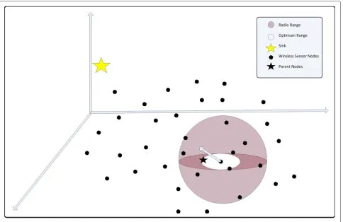
It is assumed that the nodes are deployed in a static sce-nario and in a uniform randomly distributed manner. All nodes are in the same spherical transmission range (Fig. 1) and are identical, and every node knows its own location. The location of each node is represented in a Cartesian coordinate system (X,Y,Z) which can be obtained from the GPS module. The GPS module calculates the posi-tion of each node, and it will be used only at the time of deployment; after that, it will be switched off to save energy [23]. The goal of the proposed protocols is to min-imize the RF range based on the parent location. Figure 1 is a graphical vision of 3DPBARP scenario and shows the parent selecting in this protocol. After parent selection in PFR, the position of the parents is sent to its entire chil-dren. The PFR technique in 3DPBARP uses the position’s data to minimize the RF range. The RF range is calcu-lated in location management phase, and the transponder of the node sets the transponder power to cover only the
minimized RF range that is calculated based on node and parent locations.
The location management phase is one of the key factors in 3DPBARP. The PFR is calculated in location manage-ment phase to ideally contain minimum forwarding nodes to limit the number of retransmitting nodes in a group of one-hop neighbours. In PFR, the parent location is denoted as (Xp,Yp,Zp), and the node location is denoted as (Xn,Yn,Zn).
The parent location information is provided to nodes during the parent selection mechanism. Then, the neigh-bours’ node calculates the distance from the node to its parent. In the forwarding management phase, to avoid redundant packet transmission in the network, the transponder power is set to cover only the minimum transmission distance (MTD).
MTD=
(Xp−Xn)2+(Yp−Yn)2+(Zp−Zn)2 (1)
where(Xp,Yp,Zp)denotes the position of the parent and (Xn,Yn,Zn)denotes the position of the node. Each node selects its parent from a group of qualified neighbours that have already advertised their minimum root distance (MRD) values. The neighbour that is selected as the node’s parent is the neighbour with the least MRD value. The
Fig. 2Rainbow colouring technique
second goal of the proposed protocols is to use the Rain-bow mechanism to solve VNP to enhance the reliability of the protocol and increase the packet delivery ratio. The proposed protocol has three main functionalities: parent selection that selects the best parent from the qualified neighbours of the node, location management that calcu-lates the position of each node and the minimum radius of RF range, and the VNP handling that avoids forwarding the packets toward the hole or dead end.
3.3 Parent selection in 3DPBARP
A few nodes in the network advertise themselves as sink. Other nodes in the network form a tree network
topology and send data toward these root nodes. Each node chooses the path to root by selecting the next hop based on a routing gradient [11]. 3DPBARP uses surface distance (SD) as its routing gradient. Each node is labelled as a MRD value. Root MRD value is 0, and others nodes’ value is calculated by formula 2:
Node(MRD)=Parent(MRD)+Link(SD) (2)
Link(SD)=
(Xp−X)2+(Yp−Y)2+(Zp−Z)2 (3)
where Link(SD) denotes the surface distance of the node,(Xp,Yp,Zp)denotes the position of the parent and (X,Y,Z) denotes the position of the node. Each node selects its parent from a group of qualified neighbours that have already advertised their MRD values. The neighbour that is selected as the node’s parent is the neighbour with the least MRD value.
3.3.1 Rainbow mechanism in 3DPBARP
In this section, the Rainbow mechanism has been consid-ered, and how it is used in 3DPBARP to avoid dead end routes is demonstrated.
The principle of Rainbow is to forward the packets toward the sink. In this mechanism, every node has a colour code based on how far it is from the sink. The order list of colour shows how, by selecting a node, the next relay node could travel toward the sink. LetCk(i)be the
colour code of nodei, and nodeiwill forward only to the next relay nodes with a colour code equal toCk−1orCk.
It will guarantee that the packets travel toward the sink and it avoids sending the packets toward dead end routes. Figure 2 shows how the nodes select their parents based
on the Rainbow mechanism. Each node selects its parents with its colour code or with a colour code in order to be close to the sink.
The colour code in each node is calculated based on a counter. The rainbow counter is the number of received packets from the sink. Any node with higher value of this
counter shows that it is closer to the sink than other nodes with lower value.
3.4 Loop avoidance in 3DPBARP
3DPBARP uses a detection mechanism during the data packet transmission to validate the routing path and topology. This mechanism makes 3DPBARP avoid loops by checking the previous N(l) nodes where a packet comes through. If the current node is in the list of N(l) last nodes, a network loop will occur and reconsidering the topology will be needed to put it in order.N(l)sets in the initiate stage.
4 Evaluation system model
System evaluation has been performed through massive simulations. Omnet++ has been used as a WSN simu-lator, and MATLAB has been used for simulating the energy model. Each scenario runs more than 20 times to collect the reliable results with confidence intervals of 0.95.
4.1 System channel model
The simulations run on a field area of 200×200×100 m, and the radio feature CC2420 has been used as radio module that is working on IEEE 802.15.4 standard [24]. Simulations have been run from 18 up to 3000 s. The vari-ety of radio channel has been set up by ‘Wireless Channel Sigma’ that is 0, 1, 3, and 5. Wireless Channel Sigma shows the standard deviation of the communication chan-nel diversity [25]. The received signal strength at a wireless node in real scenarios depends not only on distance from the transmitter but also on shadowing effects. The sigma parameters represent the random shadowing effects in the wireless channel parameters.
The Radio Collision Model has been selected as the one that puts more collision than normal.
4.2 Energy consumption model
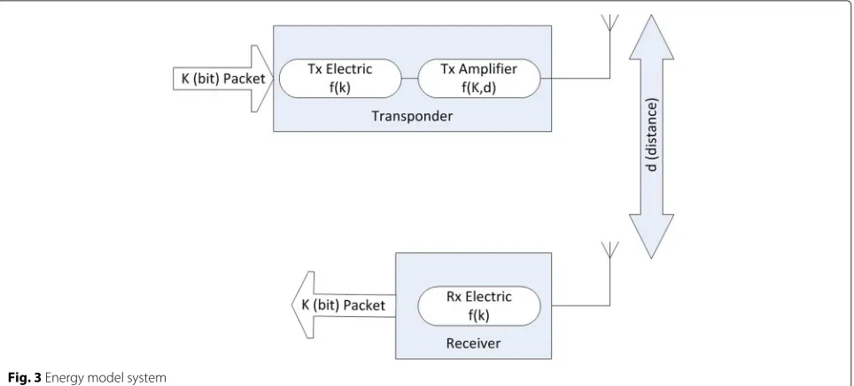
The energy consumption models are compared by a study in [26] that shows the components that consume energy in WSNs. In this paper, it has been assumed that the power energy that is consumed is mostly derived by the RF mod-ule for transmission signals which are involved in sending and receiving packets in wireless sensor nodes (Fig. 3).
Following the researches in [27–29], the mathemati-cal model for energy consumption by transmitting and receiving packets per bits of each sensor node is calculated as follows. The energy consumption in the RF module in the receiver is given as
ERx(k)=Eelec×k (4)
whereERxis the energy consumption in the receiver node,
Eelec is the energy required to process 1 bit in the elec-tronic modules andkis the length of the message (bit); the
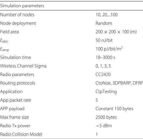
Table 1Omnet ++ simulation parameters
Simulation parameters
Number of nodes 10, 20,...100
Node deployment Random
Field area 200×200×100 (m)
Eelec 50 nJ/bit
Eamp 100 pJ/bit/m2
Simulation time 18–3000 s
Wireless Channel Sigma 0, 1, 3, 5
Radio parameters CC2420
Routing protocols CtoNoe, 3DPBARP, DFRP
Application CtpTesting
App packet rate 5
APP payload Constant 150 bytes
Max frame size 2500 bytes
Radio Tx power −5 dBm
Radio Collision Model 1
energy consumption in the transmitter RF module is given as
ETx(k,d)=Eelec×k+Eamp×k×d2 (5)
where ETx is the energy consumption in the transmit-ter node, Eamp is the energy required to transmit 1 bit in the RF module, k is the length of the message (bit) andddenotes the distance between the transmitter and receiver measured in metres. Figure 3 is a graphical vision of energy model system and shows the elements of this model.
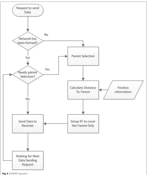
Figure 4 shows the flow chart of the 3DPBRP algorithm. It shows how each packet is sent, and it checks the sta-tus of the parent; if the protocol needs to go to the parent selection mechanism, then it selects a new parent and then sets the RF to a range that covers only this new parent.
Fig. 6Packet delivery ratio and Number of Nodes in 3DPBRP, 3DPBARP and DFRP
5 Performance evaluation
The results have been collected in different scenarios with different numbers of nodes in the field, RF range and the number of packets with confidence intervals of 0.95. In this experience, 3DPBRP as a 3D and position-based ver-sion of the CTP, 3DPBARP and Directed Flooding Routing Protocol (DFRP) have been compared. Table 1 shows the parameters of simulations. Omnet++ has been employed as a simulation to measure packet delivery ratio (PDR) and delay. End-to-end delay has been measured in all three routing protocols and also PDR. MATLAB has been used for simulating the energy model. The total energy, number of retransmitted messages and also numbers of received messages in different scenarios have been investigated in this research. The scenarios contain different wireless nodes in the field, different RF ranges and also different numbers of messages.
Fig. 7Number of retransmission messages and number of transmissions in 3DPBRP, 3DPBARP and DFRP
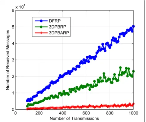
Fig. 8Number of received messages and number of transmissions in 3DPBRP, 3DPBARP and DFRP
The application layer measures the level of packet latency (in ms). Figure 5 shows the packet delivery delay level in three routing protocols: 3DPBRP, 3DPBARP and DFRP. The results show that 3DPBARP has better perfor-mance than 3DPBRP and also DFRP in terms of packet delivery delay. 3DPBARP has delivered on average about 35 % of packets in less than 20 ms compared to 3DPBRP which delivered about 26 %. It is obvious that 3DPBARP has better performance than 3DPBRP in terms of packet delivery delay time.
The application layer also measures the percentage of packet delivery ratio showing the amount of packets that were successfully received in their destinations. Figure 6 shows the packet delivery ratio in three routing proto-cols. The results show that 3DPBRP and 3DPBARP have
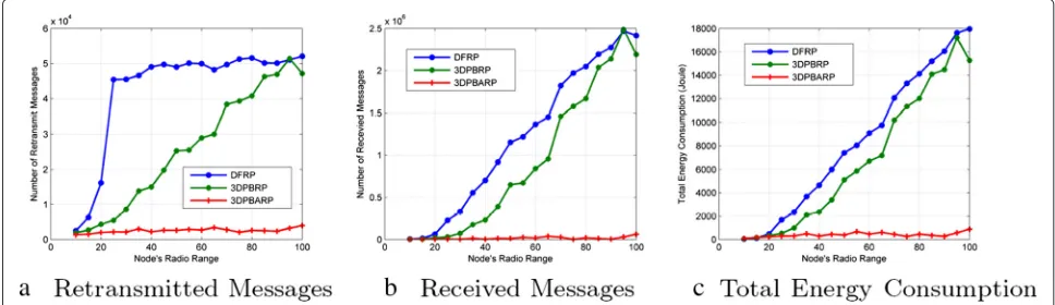
Fig. 103DPBARP, 3DPBRP and DFRP in scenarios with different numbers of nodes.aRetransmitted messages,breceive messages andctotal energy consumption
the same result in terms of packet delivery ratio in sce-narios that wireless nodes are less than 70 nodes. When the number of nodes in the fields increases to 70 nodes, it is obvious that 3DPBARP could deliver more packets than 3DPBRP. In a scenario with 100 nodes in the fields, packet delivery ratio in 3DPBARP is 55 % and 3DPBRP could manage to deliver around 47 % of the packets. Figure 7 shows the number of retransmitted messages in different numbers of message scenarios. On average, the 3DPBARP retransmits messages 82 % less than DFRP and 48 % less than 3DPBRP. Figure 8 shows the num-ber of received messages in different numnum-bers of message scenarios. On average, the 3DPBARP retransmits mes-sages 88 % less than DFRP and 66 % less than 3DPBRP. Figure 9 shows the total energy consumption in differ-ent numbers of message scenarios. On average, 3DPBARP consumed energy 87 % less than DFRP and 61 % less than 3DPBRP.
Figure 10 shows the number of received and retrans-mitted messages and also the total energy consumption in different numbers of nodes in the field. Figure 11 shows the number of received and retransmitted messages
and also the total energy consumption in different radio frequency ranges in the field.
6 Conclusions
This paper proposed 3DPBARP as an Energy Efficient Rainbow Collection Routing Protocol. 3DPBARP has shown a performance improvement in packet delivery parameters. 3DPBARP performs with more accuracy by using a new parent selection and Rainbow mechanisms to choose the parents with more accuracy. It also employs techniques to avoid loops in the topology. 3DPBARP as a GRP decreases the RF range in each node by reduc-ing the number of nodes which receive the signal, usreduc-ing a new PFR technique. Nodes reduce the RF range to cover their parents only and not any nodes with further distance in the location management phase and PFR. A massive simulation on 3DPBARP shows a significant improvement in performance regarding energy consumption compared to 3DPBRP and DFRP in different scenarios. 3DPBARP shows that it could save more than 80 % of the total energy consumption in the network by using the special tech-nique in PFR. It also provides better performance in busy
and noisy environments in terms of packet delivery time and the ratio of successful packet delivery.
Competing interests
The authors declare that they have no competing interests.
Received: 4 March 2015 Accepted: 4 June 2015
References
1. Y Song, Y Chai, F Ye, W Xu, inKnowledge Engineering and Management. A novel Tinyos 2.x Routing Protocol with load balance named CTP-TICN (Springer, 2012), pp. 3–9
2. W Yi-Zhi, Q Dong-Ping, H Han-guang, inGLOBECOM Workshops (GC
Wkshps), 2011 IEEE. Pareto Optimal Collection Tree Protocol for industrial
monitoring WSNs (IEEE, 2011), pp. 508–512
3. J Zhao, L Wang, W Yue, Z Qin, M Zhu, inMobile Ad-hoc and Sensor Networks
(MSN), 2011 Seventh International, Conference on. Load migrating for the
hot spots in wireless sensor networks using CTP (IEEE, 2011), pp. 167–173 4. F Entezami, C Politis, An analysis of routing protocol metrics in wireless
mesh networks. J. Commun. Netw. IEEE.4(12), 15–36 (2014)
5. PA Levis, N Patel, D Culler, S Shenker,Trickle: A Self-Regulating Algorithm for Code Propagation and Maintenance in Wireless Sensor Networks
6. O Gnawali, Fonseca R, K Jamieson, D Moss, P Levis, inProceedings of the
7th ACM Conference on Embedded Networked Sensor Systems. Collection
Tree Protocol (ACM, 2009), pp. 1–14
7. N Chilamkurti, S Zeadally, A Vasilakos, V Sharma, Cross-layer support for energy efficient routing in wireless sensor networks. J. Sensors.2009 (2009). Hindawi Publishing Corporation
8. Y Zeng, K Xiang, D Li, AV Vasilakos, Directional routing and scheduling for green vehicular delay tolerant networks. Wireless Netw.19(2), 161–173 (2013)
9. C Petrioli, M Nati, P Casari, M Zorzi, S Basagni,ALBA-R: load-balancing
geographic routing around connectivity holes in wireless sensor networks.
(IEEE)
10. S Al Rubeaai, B Singh, M Abd, K Tepe, inSENSORS, 2013 IEEE. Region based three dimensional real-timel routing protocol for wireless sensor networks, (Nov 2013), pp. 1–4. ISSN 1930–0395
11. M Li, Z Li, AV Vasilakos, A survey on topology control in wireless sensor networks: taxonomy, comparative study, and open issues. Proc. IEEE. 101(12), 2538–2557 (2013)
12. J Flathagen, E Larsen, PE Engelstad, O Kure, inLocal Computer Networks
Workshops (LCN Workshops), 2012 IEEE 37th Conference on. O-CTP: hybrid
opportunistic collection tree protocol for wireless sensor networks (IEEE, 2012), pp. 943–951
13. F Entezami, M Tunicliffe, C Politis, Find the weakest link statistical analysis on wireless sensor network link-quality metrics. Veh. Technol. Mag. IEEE. 9(3), 28–38 (2014)
14. Y Li, H Chen, R He, R Xie, S Zou, inWireless Communications and Signal
Processing (WCSP), 2010 International Conference on. ICTP: an improved
data collection protocol based OnCTP (IEEE, 2010), pp. 1–5
15. J Zhao, L Wang, W Yue, Z Qin, M Zhu, inMobile Ad-hoc and Sensor Networks
(MSN) 2011 Seventh International Conference on. Load migrating for the
hot spots in wireless sensor networks using CTP, (2011), pp. 167–173 16. O Chipara, Z He, G Xing, Q Chen, X Wang, C Lu, J Stankovic, T Abdelzaher,
inQuality of Service, 2006. IWQoS 2006. 14th IEEE International Workshop on.
Real-time power-aware routing in sensor networks, (2006), pp. 83–92. doi:10.1109/IWQOS.2006.250454, ISSN 1548–615X
17. F Cadger, K Curran, J Santos, S Moffett, A survey of geographical routing in wireless ad-hoc networks. Commun. Surv. Tutorials IEEE.15(2), 621–653 (2013)
18. T He, J Stankovic, T Abdelzaher, C Lu, A spatiotemporal communication protocol for wireless sensor networks. Parallel Distributed Syst IEEE Trans. 16(10), 995–1006 (2005)
19. E Felemban, C-G Lee, E Ekici, MMSPEED: multipath multi-speed protocol for QoS guarantee of reliability and timeliness in wireless sensor networks. Mobile Comput. IEEE Trans.5(6), 738–754 (2006)
20. A Ahmed, N Fisal, A real-time routing protocol with load distribution in wireless sensor networks. Comput. Commun.31(14), 3190–3203 (2008)
21. G Kao, T Fevens, J Opatrny, inWireless Pervasive Computing, 2007. ISWPC
’07. 2nd International Symposium on. 3-D localized position-based routing
with nearly certain delivery in mobile ad hoc networks, (Feb. 2007). doi:10.1109/ISWPC.2007.342627
22. P Li, S Guo, S Yu, AV Vasilakos, inINFOCOM, 2012 Proceedings IEEE. CodePipe: an opportunistic feeding and routing protocol for reliable multicast with pipelined network coding (IEEE, 2012), pp. 100–108 23. F Entezami, TA Ramrekha, C Politis, inComputer Aided Modeling and
Design of Communication Links and Networks (CAMAD), 2012 IEEE 17th
International Workshop on. An enhanced routing metric for ad hoc
networks based on real time testbed (IEEE, 2012), pp. 173–175 24. JT Adams, inAerospace Conference, 2006 IEEE. An introduction to IEEE STD
802.15.4, (2006), p. 8
25. F Entezami, C Politis, inWireless Communications and Networking
Conference Workshops (WCNCW), 2014, IEEE. Deploying parameters of
wireless sensor networks in test bed environment, (April 2014), pp. 145–149
26. MC Liu, H Chen, inProc Conf. Dependable Computing, Yichang, China. A survey of wireless sensor networks, vol. 2, (Jan. 2000), p. 10.
doi:10.1109/HICSS.2000.926982
27. Y Li, G Xiao, G Singh, R Gupta, Algorithms for finding best locations of cluster heads for minimizing energy consumption in wireless sensor networks. Clustering Algorithms; Energy Efficiency; Free-Space Model; Multipath Model; Wireless Sensor Networks. Wireless Netw.19, 1755–1768 (2013)
28. S Lindsey, C Raghavendra, K Sivalingam, Data gathering algorithms in sensor networks using energy metrics. Parallel Distributed Syst. IEEE Trans. 13(9), 924–935 (2002)
29. W Heinzelman, A Chandrakasan, H Balakrishnan, inSystem Sciences, 2000.
Proceedings of the 33rd Annual Hawaii International Conference on.
Energy-efficient communication protocol for wireless microsensor networks, vol. 2, (Jan. 2000), p. 10. doi:10.1109/HICSS.2000.926982
Submit your manuscript to a
journal and benefi t from:
7Convenient online submission 7Rigorous peer review
7Immediate publication on acceptance 7Open access: articles freely available online 7High visibility within the fi eld
7Retaining the copyright to your article