Distributed stochastic power control in ad hoc networks: a nonconvex optimization case

(1)

R E S E A R C H

Open Access

Distributed stochastic power control in ad hoc

networks: a nonconvex optimization case

Lei Yang

1*

, Yalin E Sagduyu

2

, Junshan Zhang

1

and Jason H Li

2

Abstract

Signal-to-interference-plus-noise-based power allocation in wireless ad hoc networks is inherently a nonconvex optimization problem because of the global coupling induced by the co-channel interference. To tackle this challenge, we ﬁrst show that the globally optimal point lies on the boundary of the feasible region. This property is utilized to transform the utility maximization problem into an equivalent max–min problem with more structure. By using extended duality theory, penalty multipliers are introduced for penalizing the constraint violations, and the minimum weighted utility maximization problem is then decomposed into subproblems for individual users to devise a distributed stochastic power control algorithm, where each user stochastically adjusts its target utility to improve the total utility by simulated annealing (SA). The proposed distributed power control algorithm can guarantee global optimality at the cost of slower convergence due to SA involved in the global optimization. The geometric cooling scheme with suitable choice of penalty parameters is then used to improve the convergence rate. Next, by

integrating the stochastic power control approach with the back-pressure algorithm, we develop a joint scheduling and power allocation policy to stabilize the queueing systems under random packet traﬃc. Finally, we generalize the above distributed power control algorithms to multicast communications, and show their global optimality for multicast traﬃc.

Keywords: Distributed power control, Nonconvex optimization, Extended duality theory, Simulated annealing, Queue stability, Unicast communications, Multicast communications

Introduction

The broadcast nature of wireless transmissions makes wireless networks susceptible to interference, which dete-riorates quality of service (QoS) provisioning. Power con-trol is considered as a promising technique to mitigate interference. One primary objective of power control is to maximize the system utility that can achieve a variety of fairness objectives among users [1-4]. However, maxi-mizing the system utility, under the physical interference model, often involves nonconvex optimization and it is known to be NP-hard, due to the complicated coupling among users through mutual interference eﬀects [5].

Due to the nonconvex nature of the power control prob-lem, it is challenging to ﬁnd the globally optimal power allocation in a distributed manner. Notably, the authors of

*Correspondence: [email protected]

1School of ECEE, Arizona State University, Tempe, AZ 85287, USA Full list of author information is available at the end of the article

[6-9] devised distributed power control algorithms to find power allocations that can only satisfy the local optimality conditions, but global optimality could not be guaran-teed in general, except for some special convexifiable cases (e.g., with strictly increasing log-concave utility func-tions). Another thread of work applied game-theoretic approaches to power control by treating it as a non-cooperative game among transmitters [10,11]. However, distributed solutions that converge to a Nash equilibrium may be suboptimal in terms of maximizing the total sys-tem utility. Different from these approaches, the authors of [12] transformed the power control problem into a DC (difference of convex functions) optimization prob-lem [13]. Then, the global optimal solution can be solved in a centralized manner with the branch-and-bound algo-rithm. Recent study [14] proposed a globally optimal power control scheme, named MAPEL, by exploiting the monotonic nature of the underlying optimization prob-lem. However, the complexity and the centralized nature

(2)

of MAPEL hinder its applicability in practical scenarios, and thus it can be treated rather as a benchmark for performance evaluation in distributed networks.

To ﬁnd the globally optimal power allocation in a distributed setting, recent study [15] has proposed the SEER algorithm based on Gibbs sampling [16], which can approach the globally optimal solution in an asymptotic sense when the control parameter in Gibbs sampling tends to inﬁnity. Notably, for each iteration in the SEER algo-rithm, each user utilizes Gibbs sampling to compute its transition probability distribution for updating its trans-mission power, where the requirement for message pass-ing and computpass-ing the transition probability distribution in each iteration can be demanding when applied to ad hoc communications without centralized control.

A challenging task in distributed power control in ad hoc networks is to reduce the amount of message pass-ing while preservpass-ing the global optimality. To tackle this challenge, we ﬁrst show that the globally optimal point lies on the boundary of the feasible region. This property is utilized to transform the utility maximization problem into an equivalent max–min problem with more struc-ture, which can be solved by combining recent advances in extended duality theory (EDT) [17] with simulated annealing (SA) [18]. Compared with the classical dual-ity theory with nonzero dualdual-ity gap for nonconvex opti-mization problems, EDT can guarantee zero duality gap between the primal and dual problems by utilizing non-linear Lagrangian functions. This property allows for

solv-ing the nonconvex problem by its extended dual while

preserving the global optimality with distributed imple-mentation. Furthermore, as will be shown in Section “Power control for unicast communications”, for the sub-problem of each individual user, the extended dual can then be solved through stochastic search with SA. In particular, we ﬁrst transform the original utility maxi-mization problem into an equivalent max–min problem. This step is based on the key observation that in the case with continuous and strictly increasing utility functions,

the globally optimal solution is always on the boundary

of the feasible (utility) region. Then, appealing to EDT and SA, we develop a distributed stochastic power con-trol (DSPC) algorithm that stochastically searches for the optimal power allocation in the neighborhood of the fea-sible region’s boundary, instead of bouncing around in the entire feasible region.

Speciﬁcally, we ﬁrst show that DSPC can achieve the global optimality in the underlying nonconvex optimiza-tion problem, although the convergence rate can be slow (but this is clearly due to the slow convergence nature of SA with logarithmic cooling schedule). Then, to improve the convergence rate of DSPC, we propose an enhanced DSPC (EDSPC) algorithm that employs the geometric cooling schedule [19] and performs a careful selection

of penalty parameters. As a benchmark for performance evaluation, we also develop a centralized algorithm to search for the globally optimal solution over simplices that cover the feasible region. The performance gain is further veriﬁed by comparing our distributed algorithms with MAPEL [14], SEER [15], and ADP [6] algorithms. Worth noting is that the proposed DSPC and EDSPC algorithms do not require any knowledge of channel gains, which is typically needed in existing algorithms, and instead they need only the standard feedback of signal-to-interference-plus-noise (SINR) for adaptation.

Next, we integrate the proposed distributed power con-trol approach with the back-pressure algorithm [20] and devise a joint scheduling and power allocation policy for improving the queue stability in the presence of dynamic packet arrivals and departures. This policy fits into the dynamic back-pressure and resource allocation frame-work and enables distributed utility maximization under stochastic packet traffic [21,22]. Then, we generalize the study to consider multicast communications, where a sin-gle transmission may simultaneously deliver packets to multiple recipients [23,24]. Specifically, we extend DSPC and EDSPC algorithms to multicast communications with distributed implementation, and show that these algo-rithms can also achieve the global optimality in terms of jointly maximizing the minimum rates on bottleneck links in different multicast groups.

The rest of the article is organized as follows. In the following section, we ﬁrst introduce the system model, establish the equivalence between the utility maximiza-tion problem and its max–min form, and then develop both centralized and distributed algorithms for the max– min problem. Next, building on these power control algo-rithms, we develop in Section “Joint scheduling and power control for stability of queueing systems” a joint schedul-ing and power allocation policy to stabilize queueschedul-ing sys-tems. The generalization to multicast communications is presented in Section “Power control for multicast com-munications”. We conclude the article in “Conclusion” Section.

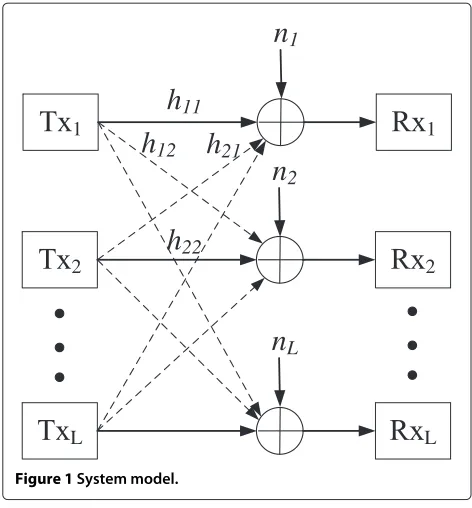
Power control for unicast communications System model

We consider an ad hoc wireless network with a setL =

{1,. . .,L} of links, where the channel is

interference-limited, and all L links treat interference as noise, as

(3)

1 1

2 2

L L

n

1

n

₂

n

L

h

11

h

12

h

₂₂

h

₂₁

Figure 1System model.

γ_l(p)= hllpl nl+

k=l hklpk

, (1)

wherep = (p1,. . .,pL)is a vector of the users’ transmis-sion powers andnlis the noise power. Accordingly, thelth user receives the utilityUl(γl), whereUl(·)is continuous and strictly increasing. We assume that each userl’s utility is zero whenγl =0, i.e.,Ul(0)=0. For ease of reference, the key notation of this article is listed in Table 1.b

Table 1 Summary of the notations and deﬁnitions

Notation Deﬁnition

L Set of links

L Total number of links

hlk Channel gain from linkl’s transmitter to linkk’s receiver

H Link gain matrix

pl(in vectorp) Transmission power of linkl

nl(in vectorn) Noise power for linkl

γl SINR of linkl

γl(·) SINR function of linkl

Ul(·) Utility function of linkl

xl(in vectorx) Ratio of linkl’s utility to the total network utility

rl(in vectorr) Transmission rate of linkl

rl(·) Transmission rate function of linkl

α,β Penalty multipliers

Network utility maximization

We seek to ﬁnd the optimal power allocationp∗that max-imizes the overall system utility subject to the individual power constraints, given by the following optimization problemc:

maximize

l∈LUl

(γ_l(p))

subject to 0≤pl≤Pmax_l ,∀l∈L variables {p}.

(2)

In general, (2) is a nonconvex optimization problem.d In particular, if the utility function is the Shannon rate achievable over Gaussian ﬂat fading channels, namely

Ul(γl(p)) = wllog(1+γl(p)), wherewl > 0 is a weight associated with userl, (2) boils down to the weighted sum rate maximization problem, which is known to be non-convex and NP-hard [5]. Note that the weights in (2) can serve as the fairness measures [25] for diﬀerent scenar-ios. In particular, in queueing systems, packet queues for arrival rates within the stability region can be stabilized by solving this weighted sum rate maximization prob-lem, where the instantaneous queue lengths are chosen as the weights. In Section “Joint scheduling and power control for stability of queueing systems”, we will discuss how to stabilize the packet queues by integrating our dis-tributed power control algorithms with the back-pressure algorithm.

LetF denote the feasible utility region, where for each pointU = (U1,. . .,UL)in F, there exists a power vec-torpsuch thatUl = Ul(γl(p))for alll ∈ L. The feasible utility regionFis nonconvex, and in general, ﬁnding the globally optimal solution to (2) inFis challenging. In the following example, we illustrate the geometry ofFfor the utility functionUl(γl(p))=wllog(1+γl(p))and evaluate the solutions to (2) given by some existing power control approaches discussed in Section “Introduction”.

Example.For the case with two links, Figure 2 illustrates the nonconvex feasible utility regionF for diﬀerent sys-tem parameters. We compare the performance of the existing approaches [3,6,14,15] in Table 2.

Remarks.The solutions to (2) given by the authors of [3,6,14] are either distributed but suboptimal or optimal but centralized. In particular, Chiang et al. [3] solve (2) by using geometric programming (GP) under the high-SINR assumption, which yields a suboptimal solution to (2) when this assumption does not hold (e.g., this is the case in the example above). The ADP algorithm [6] can

guarantee only local optimalitye in a distributed

(4)

0 1 2 3 4 5

Figure 2The feasible utility region_F.Case (I): the channel gains are given byh11=0.73,h12=0.04,h21=0.03, andh22=0.89, and the maximum power arePmax

1 =20,Pmax2 =100; Case (II): the channel gains are given byh11=0.30,h12=0.50,h21=0.03, and

h22=0.80, and the maximum power arePmax1 =1,Pmax2 =2. In both cases, the noise power is 0.1 for each link, and the weights are w1=0.57,w2=0.43.

the SEER algorithm [15] can guarantee global optimality in a distributed manner but message passing needed in each iteration can be demanding, i.e., each link needs the knowledge of the channel gains, the receiver SINR and the signal power of all the other links. It is worth noting that the performance of SEER hinges heavily on the control parameter that can be challenging to choose on the ﬂy.

From network utility maximization to minimum weighted utility maximization

In order to devise low-complexity distributed algorithms that can guarantee global optimality, we ﬁrst study the basic properties for the solutions to (2), before transform-ing (2) into a more structured max–min problem.

Lemma 1.The optimal solution to (2) is on the boundary of the feasible utility regionF.

Table 2 The performance of the existing approaches for Case I and II

Approach Case I Case II

Power Sum rate Power Sum rate

GP [20, 7.68] 3.02 [1, 0.61] 0.98

ADP [20, 6.46] 3.10 [1, 2] 1.16

MAPEL [20, 6.79] 3.10 [0, 2] 1.22

SEER [20, 6.90] 3.10 [0, 2] 1.22

Proof. Let U∗ denote a globally optimal solution to (2)

overF, andγ∗denote the corresponding SINR that

sup-portsU∗. SinceUl(·)is continuous and strictly increasing, proving thatU∗is on the boundary ofF is equivalent to

showing thatγ∗is on the boundary of the feasible SINR

region. Suppose thatγ∗is not on the boundary of the fea-sible SINR region, which indicates that there exists some pointγˆ such thatγˆl ≥ γ_l∗for alll ∈ Landγˆl > γ_l∗ for

somel ∈ L. SinceUl(·)for anyl ∈ Lis strictly increas-ing in γ_l, we have Ul(γˆl) ≥ Ul(γ_l∗) for all l ∈ L and Ul(γˆl) > Ul(γ_l∗)for somel ∈ L, which contradicts the

fact thatγ∗is a globally optimal solution. Hence, Lemma 1 follows.

Based on Lemma 1, if we can characterize the boundary ofF, then it is possible to solve (2) eﬃciently. Thus moti-vated, we ﬁrst establish, by introducing a “contribution weight” for each user, the equivalence between (2) and the minimum weighted utility maximization problem.

Lemma 2.Problem (2) is equivalent to the following minimum weighted utility maximization:

xl . Therefore, (4) can be treated as the

hypograph form of (3), i.e., (4) and (3) are equivalent [26], thereby concluding the proof.

(5)

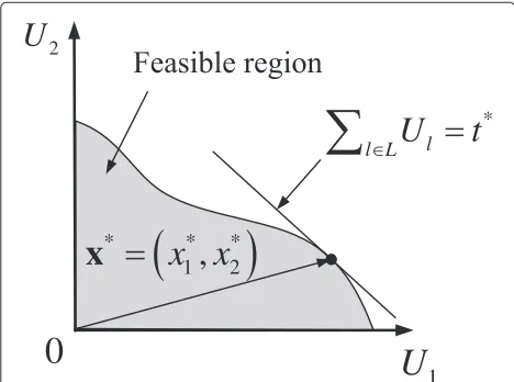
optimalx∗, given which we can efficiently obtain a globally optimal solution, i.e., the tangent point of the hyperplane andF, as illustrated in Figure 3. Intuitively speaking, x represents a search direction. Once we find the best search directionx∗,p∗ can be obtained efficiently by searching along the direction ofx∗. Actually, for givenx, (3) is quasi-convex.fBy introducing an auxiliary variablet, we obtain the following equivalent formulation:

maximize t

subject to U_l−1(txl)(nl+ k=l

hklpk)≤hllpl

0≤pl ≤Pmax_l ,∀l∈L, 0≤t variables {p,t},

(5)

which can be solved in polynomial time through binary

search ont [26]. However, the optimal search direction

x∗ is diﬃcult to ﬁnd due to the nonconvex nature of the

problem. In the following section, we study how to ﬁnd the globally optimal search directionx∗.

Centralized versus distributed algorithms

In this section, we study algorithms achieving global opti-mality for (3). First, we propose a centralized algorithm for (3), which will serve as a benchmark for performance comparison. Then, by using EDT and SA, we propose a distributed algorithm, DSPC, for the problem (3). Build-ing on this, we propose an EDSPC algorithm to improve the convergence rate of DSPC.

A centralized algorithm

Based on Lemmas 1 and 2, we develop a centralized algo-rithm (Algoalgo-rithm 1) to solve the max–min optimization problem (3) under consideration. Roughly speaking, by dividing the simplexS= {x|_l_∈_Lxl=1, 0≤xl ≤1,∀l∈

L}into many small simplices, the algorithm can ﬁnd the

optimal point on the boundary ofF. Figure 4 illustrates

0

2

U

1

U

* l

l L

U

t

* * *

1

,

2

x x

x

Figure 3An illustration of the max–min problem for the case with two links.

If

S

c

v

S

1 S

S

₂

Figure 4An illustration of the simplex cutting for the case with three links.

how the simplex cutting is performed for the case with three links. Compared with the MAPEL algorithm [14], Algorithm 1 directly computes the points on the bound-ary, instead of constructing a series of polyblocks to approximate the boundary of the feasible region.

Algorithm 1

Initialization: Choose the approximation factor > 0,

and construct the initial simplex S with the vertex set

V = {v1,. . .,vL}, where vl = el and el is the lth unit coordinate vector. Letvc = 1_Ll∈Lvlbe the center ofS. Computep∗by solving (5) at the point x = vc. Denote

δ(S)=maxv∈V|vc−v|as the diameter ofS. Repeat

1. Divide each simplexSiby usingbisection method, which chooses the midpoint of one of the longest edges of the simplexSi, i.e.,vm= ₂1(vr+vs), where vrandvsare the end points of a longest edge of the simplex. In this case, the simplexSiis subdivided into two simplicesSi1andSi2.

2. For each new simplexSij, compute the diameter

δ(Sij)andp∗by solving (5) atxgiven by the center point of the simplex.

3. Find the current best solution to (3) and the maximal diameterδmin these new subdivided simplices.

Untilδm< .

Proposition 1.Algorithm 1 converges monotonically to the globally optimal solution to (3) as the approximation factorapproaches zero.

(6)

Letd()denote the maximum distance between the opti-mal solutionx∗and the center point of the simplex that

contains x∗. Obviously, d() is bounded by δm. Since

δm decreases with the decreasing of , therefore d()

decreases monotonically with the decreasing of, i.e., the solution given by Algorithm 1 monotonically converges

to x∗. As approaches zero, Algorithm 1 exhaustively

searches every point in the simplexS, thereby concluding the proof.

Remarks. Algorithm 1 can be used to obtain an-optimal solution with |x−x∗| ≤ . That is to say, by

control-ling , one can strike a balance between the optimality

and the computation time. Since ﬁnding the globally opti-mal solution requires centralized implementation, Algo-rithm 1 will be used only as a benchmark for performance evaluation of distributed algorithms.

DSPC algorithm

Next, we devise a DSPC algorithm based on EDT [17] and SA [18]. Compared to the classical duality theory with nonzero duality gap for nonconvex optimization prob-lems, EDT can guarantee zero duality gap between the pri-mal and dual problems by utilizing nonlinear Lagrangian functions. This property allows for solving the nonconvex

problem by itsextended dualwhile preserving the global

optimality in distributed implementation. To this end, we ﬁrst introduce auxiliary variables and use EDT to trans-form (3) with the auxiliary variables into an unconstrained problem. Then, we solve the unconstrained problem by

using the SA mechanism. Speciﬁcally, we deﬁne tl =

Ul(γl(p))

xl and rewrite (3) as

minimize −min

Next, we use EDT to write the Lagrangian function for (6) as

the penalty multipliers for penalizing the constraint vio-lations. Based on EDT [17], there exist ﬁniteα∗ ≥ 0 and

β_l∗ ≥ 0, for alll ∈ L, such that, for anyα > α∗ and

β_l > β_l∗, ∀l ∈ L, the solution to (7) is the same as (6).

Note that (7) does not include the constraints ofpl,xl, and tl for each user, and there will be no constraint violation when each user updates these variables locally. Therefore, the minimization of (7) with respect to the primal vari-ables (p,x, andt) can be carried out individually by each user in a distributed fashion.

The next key step is to perform a stochastic local search by each user based on SA. Lettl,xl, andpldenote the pri-mal values of the lth user, andt_l andx_l denote the new values randomly chosen by thelth user. Accordingly,t_lx_l

can be treated as a new target utility for thelth user. To achieve this target utility, thelth user updatesp_lby

p_l =min

where γ_l is the current SINR measured at thelth user’s receiver. Note that (8) does not need any information of channel gains, except the feedback of SINR γ_l. Since (8) corresponds to the distributed power control algo-rithm of standard form as described in [27],git converges geometrically fast to the target utility. Thus, we assume

that each user l updates pl at a faster time-scale than

tl and xl such that pl always converges before the next update of tl and xl. Next, we use SA to update tl and

xl in a stochastic operation. By using the analogy with

annealing in metallurgy, SA was proposed in [18] to mimic the behavior of the microscopic constituents in heating and controlled cooling of a material. By allow-ing occasional uphill moves, SA is able to escape from

the local optimal points. In particular, let denote

the diﬀerence between L(pl,xl,tl|p−l,x−l,t−l,α,β) and L(p_l,x_l,t_l|p₋_l,x−l,t−l,α,β), where y−l is the vector y without thelth user’s variable. If≥ 0, i.e.,t_l,x_landp_l

reduce Lagrangian (7), then they are accepted with prob-ability 1; otherwise, they are accepted with probprob-ability

exp_T, whereT is a control parameter and sometimes

it is called temperature. Note that, as T decreases, the

acceptance of uphill move becomes less and less probable, and therefore a ﬁne-grained search is needed. It has been

shown that, asT approaches 0 according to alogarithmic

cooling schedule, SA converges to a globally optimal point [16,19]. To computelocally by each userl, userlneeds to broadcast the terms tl, xl and βl(tlxl − Ul(γl(p)))+, whenever any of these terms changes.

(7)

continue to transmit at maximum power [1]. If some tar-get utility is not feasible asTtends to 0, based on EDT, the current values ofαandβdo not satisfyα > α∗orβl> β_l∗ for alll∈L. Therefore, each userlalso needs to updateα

andβl. In particular, if any constraint is violated,αandβl are updated as follows:

α ← α+σ|

l∈L xl−1|,

β_l ← β_l+ _l(tlxl−Ul(γl))+, ∀l∈L, (9) whereσ and lare used to control the rate of updatingα andβ_l. A detailed description of DSPC algorithm is given in Algorithm 2.

Remarks:

(1) In Algorithm 2, each user randomly picks

t_l∈[U_lmax,U_totmax], whereU_lmaxdenotes the maximum utility of the userl when the user l transmits at the maximum power while the other users do not transmit, andU_totmax=_l_∈_LU_lmax. Note thatU_lmaxcan be computed by each user locally. Further, we assume that each user broadcastsU_lmax

before running the algorithm so thatU_totmaxis also known by each user.

(2) In practice, after initialization,αandβ_lincrease in proportion to the violation of the corresponding constraint, which may lead to excessively large penalty values. Since it is beneﬁcial to periodically scale down the penalty values to ease the

unconstrained optimization,αandβlare scaled down by multiplying with a random value (it can be chosen between 0.7 and 0.95 according to [17]), if the penalty decrease condition is satisﬁed, i.e., the maximum violation of constraints is not decreased after consecutively running Step 1 in Algorithm 2 several times, e.g., ﬁve times in [17].

(3) In Algorithm 2, each user requires the knowledge ofT and time epochs{τ₁,τ₂,. . .}to updatetlandxl, which can be determined and informed to each user oﬄine.

Algorithm 2 DSPC

Initialization: Choose >0. Letα =0,β_l =0,∀l ∈L,

and randomly choosep,xandt.

Step 1: update primal variables

Set T = T0, and select a sequence of time epochs

{τ1,τ2,. . .}in continuous time. Repeat for each userl

1. Randomly pickt_l∈[U_lmax,U_totmax]andx_l ∈[ 0, 1], and

updatep_laccording to (8).

2. Keep sensing the change ofβ_l(tlxl−Ul(γl(p)))+ broadcast by other users.

3. Compute, and acceptt_l,x_l, andp_lwith probability 1, if≥0, or with probabilityexp(_T), otherwise. 4. Broadcastt_landx_l, ift_landx_lare updated. 5. For each time epochτi, updateT=T0/log(i+1).

UntilT< .

Step 2: update penalty variables For each userl,

1. Updateαandβlaccording to (9), and scale downα andβ_l, if the penalty decrease condition is satisﬁed. 2. Go to Step 1 until no constraint is violated.

Proposition 2.The DSPC algorithm (Algorithm 2) con-verges almost surely to a globally optimal solution to (3), as temperature T in SA decreases to zero.

Proof.To show that Algorithm 2 converges almost surely to a globally optimal solution to (3), we only need to show that when α > α∗ and β_l > β_l∗ for all l ∈ L, Algo-rithm 2 can converge almost surely to a globally optimal solution to (6), since (3) is equivalent to (6), and if the solution does not satisfy the constraints of (6),α andβl will increase in proportion to the violation of the corre-sponding constraint. Since Algorithm 2 uses SA with the logarithmic cooling schedule, based on [16,19] it can con-verge almost surely to a globally optimal solution to (7), which is also a globally optimal solution to (6) based on EDT whenα > α∗andβ_l > β_l∗for alll∈ L[17]. Hence, Proposition 2 follows.

Remarks.The DSPC algorithm can guarantee global

optimality in a distributed manner without the need of channel information. In particular, it needs the informa-tion oftl andxl, and can adapt to channel variations by utilizing the SINR feedback. However, the convergence rate of DSPC is slow due to the use of logarithmic cooling schedule.

EDSPC algorithm

It can be seen from Algorithm 2 that it is critical to

ﬁnd the optimal penalty variablesαandβfor computing

(7). Moreover, a logarithmic cooling schedule is used to ensure convergence to a global optimum. To improve the convergence rate, we propose next an EDSPC algorithm by empirically choosing the initial penalty valuesα0and β₀and employing ageometric cooling schedule[18], which reduces the temperatureTin SA byT =ξT, 0< ξ <1, at each time epoch. Compared with the logarithmic

cool-ing schedule, T converges to 0 much faster under the

(8)

We note that although EDSPC converges much faster than DSPC, it may yield only near-optimal solutions. Based on EDT, we chooseα0> α∗andβ0l > β_l∗, ∀l∈L, to satisfy the optimality conditions for penalty variables. Obviously, by choosing largeα0andβ0l, these conditions can be always satisﬁed. Nevertheless, very large penalties introduce heavy costs for constraint violations such that EDSPC may end up with a feasible but suboptimal solu-tion. Therefore, the selection of initial penalty values plays a critical role in the performance of EDSPC and deserves more attention in future work. In practice, we can choose the initial penalties based on the maximum value of the constraint that is associated with each of the penalty vari-ables. This choice performs well in the simulations. For example, we can choose β₀_l = U_lmax for the constraint

tlxl≤Ul(γl(p)).

Algorithm 3 EDSPC

Initialization: Choose > 0. Let α = α0, βl = β0l, ∀l∈L, and randomly choosep,xandt.

1. Randomly pickt_l∈[U_lmax,U_totmax]andx_l∈[ 0, 1], and

updatep_laccording to (8).

2. Keep sensing the change ofβl(tlxl−Ul(γl(p)))+ broadcast by other users.

3. Compute, and acceptt_l,x_l, andp_lwith probability 1, if≥0, or with probabilityexp(_T), otherwise. 4. Broadcastt_landx_l, ift_landx_lare updated. 5. For each time epochτi, updateT =ξT.

UntilT < .

Performance evaluation

In this section, we evaluate the utility and convergence

performance of Algorithms 2 and 3 (DSPChand EDSPC).

We consider a wireless network with six links randomly

distributed on a 10-by-10 m2 square area. The channel

gainshlk are equal tod_lk−4, wheredlk represents the dis-tance between the transmitter of userland the receiver of userk. We assumeUl(γl(p)) = log(1+γl(p)),Pmaxl = 1 andnl = 10−4for alll ∈ L, and consider one randomly generated realization of channel gains given by

H=

⎡ ⎢ ⎢ ⎢ ⎢ ⎢ ⎢ ⎣

0.3318 0.0049 0.0141 0.0021 0.0016 0.0007 0.0031 0.9554 0.0063 0.0140 0.0012 0.0025 0.0155 0.0042 0.6166 0.0046 0.0108 0.0018 0.0017 0.2188 0.0340 0.6754 0.0062 0.0215 0.0020 0.0017 0.2216 0.0042 0.2955 0.0028 0.0007 0.0079 0.0254 0.2553 0.0404 0.3025

⎤ ⎥ ⎥ ⎥ ⎥ ⎥ ⎥ ⎦

.

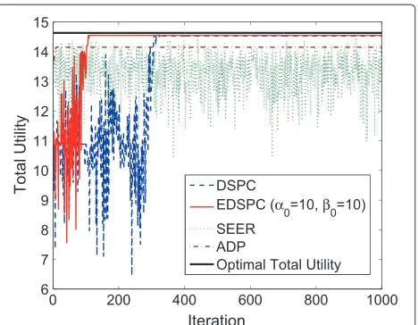
Figure 5 shows how the total utility in the EDSPC algo-rithm converges over time, when we choose all the initial

Figure 5Convergence performance of DSPC, EDSPC, SEER, and ADP.

penalty values equal to 10. Also, we chooseξ =0.9,ρ=1,

and = 1, and use Algorithm 1 as a benchmark to

eval-uate the optimal performance. As shown in Figure 5, the EDSPC algorithm approaches the optimal utility, when the initial penalty values are carefully chosen. Moreover, the convergence rate of the EDSPC algorithm is much faster than DSPC, since DSPC continues updating the penalty values even after the optimal solution is found for the current penalty values. Figure 6 illustrates the average performance (with conﬁdence interval) of DSPC, EDSPC, SEER, and ADP under 100 random initializations, with the same system parameters as used in Figure 5. As shown in Figure 6, both DSPC and EDSPC are robust against the variations of initial values.

Figures 5 and 6 compare the proposed algorithms with the SEER and ADP. As mentioned in Section “Introduc-tion”, ADP can only guarantee local optimality. There-fore, for nonconvex problems (e.g., in this example), ADP may converge to a suboptimal solution. As noted in [15], the performance of SEER heavily hinges on the control parameter that can be challenging to choose in online

DSPC EDSPC SEER ADP

0 5 10 15 20

Total Utility

(9)

operation. In contrast, DSPC can approach the glob-ally optimal solution regardless of the initial parameter selection, but the convergence rate may be slower. Fur-thermore, EDSPC improves the convergence rate, but in this case the initial penalty values would impact how close it can approach the optimal point. In terms of message passing, our algorithms do not require individual links to know the channel gains (including its own channel gain), the receiver SINR of the other links and the signal power of the other links, which are all needed in the SEER algorithm.

Joint scheduling and power control for stability of queueing systems

In Section “Power control for unicast communications”, we studied the distributed power allocation, by using DSPC and EDSPC, for utility maximization in the sat-urated case with uninterrupted packet traﬃc. In this section, we generalize the study by considering a queue-ing system with dynamic packet arrivals and departures. Speciﬁcally, we develop a joint scheduling and power allo-cation policy to stabilize packet queues by integrating our power control algorithms with the celebrated back-pressure algorithm [20].

Stability region and throughput optimal power allocation policy

Consider the same wireless network model withL links

as in Section “Power control for unicast communications”.

We assume that there are S classes of users in the

sys-tem, and that the traﬃc brought by users of classsfollows {Asl(t)}∞t=1, which arei.i.d.sequences of random variables for alll =1,. . .,Lands =1,. . .,S, whereAsl(t)denotes

the amount of traﬃc generated by users of class s that

enters the link l in slot t. We assume that the second

moments of the arrival process{Asl(t)}∞t=1are ﬁnite. Let

Qs_T₍_l₎(t) andQs_R₍_l₎(t) denote the current backlog in the queue of classsin slotton the transmitter and receiver sides of link l, respectively. The queue length Qs_T₍_l₎(t)

evolves over time as

Qs_T₍_l₎(t+1)=max(Qs_T₍_l₎(t)−rs_l(t), 0)+Asl(t)

+

{m|T(l)=R(m),m∈L}

rs_m(t), (10)

wherers_l(t)denotes the transmission rate of linklfor users of classs. The third term in (10) denotes the traﬃc from the other links. The queue length process {Qs_T₍_l₎(t)}∞_t₌₁

forms a Markov chain.

Letψs denote the ﬁrst moment of {Asl(t)}∞t=1, i.e., the load brought by users of classs. As is standard [20,21,28], the stability region is deﬁned as follows.

Deﬁnition 1.The stability region is the closure of the set of all{ψs}S_s₌₁for which there exists some feasible power allocation policy under which the system is stable, i.e., = _p_∈_P(p), where(p) = {{ψs}S_s₌1|

S

s=1Eslψs < rl(p),∀l}, P denotes the set of feasible power allocation, rl(p) denotes the rate of link l under power allocationp, and Esl=1is the indicator that the path of users of class s uses link l, and Esl=0, otherwise.

For the sake of comparison, the throughput regioniFof the corresponding saturated case is deﬁned as the set of all feasible link rates, i.e.,F = {r|rl = rl(p),p ∈ P}. In

general, the throughput regionF may be diﬀerent from

the stability region, except for some special cases (e.g., in slotted ALOHA systems the throughput region and the stability region are the same [29] for two links and in a multiple-access channel the information theoretic capac-ity region is equivalent to its stabilcapac-ity region under speciﬁc feedback assumptions [30]).

The queueing system is stable if the arrival rates of packet queues are less than the service rates such that the queue lengths do not grow to inﬁnity [31]. In order to stabilize packet queues, it is critical to ﬁnd the optimal scheduling and power allocation policy that maximizes the weighted sum rate given by (11). By integrating our power control algorithms with the back-pressure algo-rithm, we propose a joint scheduling and power allocation policy presented in Algorithm 4 to stabilize the queueing system.

Proposition 3.The joint scheduling and power allocation policy (Algorithm 4) can stabilize the system such that

lim sup_t_→∞1_tt_τ−₌1₀_l_,_sE{Qs_l(τ )} < ∞, when the traﬃc load{ψs}S_s₌₁is strictly interior to the stability region, i.e., there exists some >0such that{ψs+}S_s₌₁∈.

The proof is similar to that in [21,32], and is omitted for brevity.

Note that Algorithm 4 can be viewed as a dynamic back-pressure and resource allocation policy [32], crafted towards solving the weighted sum rate maximization problem (11). Speciﬁcally, by using the DSPC algorithm, Algorithm 4 can be implemented distributively to ﬁnd the globally optimal resource allocation. We should caution that EDSPC can be applied to improve the convergence rate of Stage 2 in Algorithm 4 but it may render a subop-timal schedule (i.e., it can not stabilize all possible{ψs}S_s₌₁

within), due to the fact that EDSPC may not always ﬁnd

the global optimal power allocation.

(10)

Algorithm 4 Joint scheduling and power allocation policy Stage 1: For each linkl, select a link weight according to wl(t) = max

s=1,...,SD s

l(t), where the diﬀerence of queue lengths of class sisDs_l(t) = max(Qs_T₍_l₎(t)−Qs_R₍_l₎(t), 0), if the receiver of linkl is not the destination of classs’s traﬃc, andDs_l(t)=Qs_T₍_l₎, otherwise.

Stage 2: Compute the optimal power allocation p∗ in

each slott by solving the following problem with DSPC

algorithm

p∗=arg max p

L

l=1

wl(t)rl(p). (11)

Thus, the transmission rate of linklin slottis given by

rl(p∗)=log(1+γl(p∗)). Stage 3:Lets∗_l =arg max

s=1,...,SDsl(t)denote the class sched-uled in slott; if multiple classes satisfy this condition, then

s∗_l is randomly chosen as one of these classes. Then, sched-ule these classes according to the solution given by Stage 2.

In this section, we present numerical results to illustrate the use of Algorithm 4 for stabilizing a queueing system. We consider a one-hop network (i.e.,E= {Esl}is the iden-tity matrix) with two users (classes), where the channel gains areh11 =0.3,h12=0.5,h21 =0.03, andh22= 0.8, and the noise power is 0.1 for each link. The maximum transmission power is set to 1 and 2 for links 1 and 2, respectively. Besides, we assume that the users of classs

arrive at the network according to a Poisson process with rateλs, and that the size of packet batch for users of class s follows an exponential distribution with meanν_s. The load brought by users of classsis thenψ_s=λ_sν_s. Figure 7

Figure 7Comparison of the stability region and the throughput region.

shows the stability region and compares it with the

throughput regionFof the corresponding saturated case.

The stability region follows from the union of link rates that are conditioned on whether the other link is back-logged or not [29,30]. First, we derive the stability region for the given power allocation. Then, we vary power allo-cation in the feasible region, and by taking the envelope of these regions, we obtain the overall stability region shown in Figure 7. However, diﬀerent from the previous cases, where the throughput region is the same as the stability region, e.g., in a slotted ALOHA system with two links [29] and in a multiple-access channel [30], the

through-put region F under the SINR model is strictly smaller

than the stability region (due to the underlying noncon-vex optimization problem), as observed from Figure 7, which is the convex hull ofF, i.e.,Co(F), achievable by timesharing across diﬀerent transmission modes.j

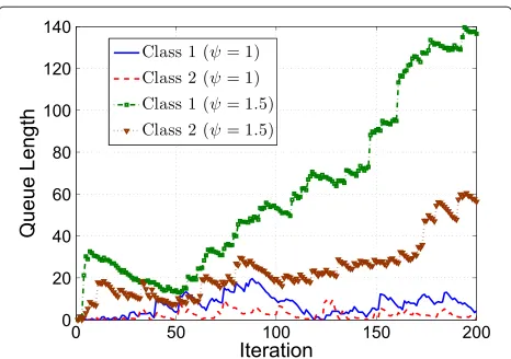
Then, we vary the arrival rateλand the average batch

sizeν to change the traﬃc intensityψ = λν. Assuming

that the arrival rate and the average batch size of each user are the same, we compare in Figure 8 the sample paths

of each user’s queue length forψ = 1 (λ = 1,ν = 1)

with ψ = 1.5 (λ = 1.5, ν = 1). Whenψ = 1, which

falls in the stability region shown in Figure 7, the system is stabilized by using Algorithm 4. On the other hand, the

system becomes unstable whenψ =1.5, which is outside

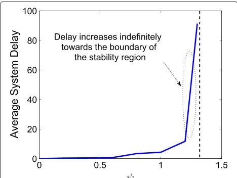
the stability region. Figure 9 illustrates the average delay of the system as a function of the arrival rates. The delay is ﬁnite for small loads and grows unbounded when the loads are outside the stability region.

Power control for multicast communications Due to wireless multicast advantage [23], multicasting enables eﬃcient data delivery to multiple recipients with a single transmission. In this section, we extend the DSPC

(11)

Figure 9Average delay of the system versus system loads .

algorithms in Section “Power control for unicast commu-nications” to support multicast communications.

System model

Beyond the model described in Section “Power control for unicast communications”, we consider that each user

lhas one transmitter and a setMlof receivers. The

cor-responding transmission rate, rl, is determined by the

bottleneck link among these transmitter–receiver pairs, i.e.,rl= min

m∈Mlrlm, whererlmdenotes the link rate between the transmitter of userland its receiverm, and it is calcu-lated from the Shannon rate log(1+γ_lm(p))for Gaussian, ﬂat fading channels. Here, we do not consider the general broadcast capacity region but rather focus on maximizing the bottleneck link rates.

Network utility maximization

We seek to ﬁnd the optimal power allocation p∗ that

maximizes the overall system utility subject to the power constraints in multicast communications, as follows:

maximize

l∈L Ul(rl)

subject to rl= min

m∈Mlrlm,∀l∈L

rlm=log(1+γlm(p)),∀l∈L,m∈Ml 0≤pl ≤Pmax_l ,∀l∈L

variables {p,{rl},{rlm}}.

(12)

Similar to (2), (12) is nonconvex due to the complicated interference coupling between individual links. Diﬀerent from the techniques used in Section “Power control for

unicast communications”, we relaxrl = min

m∈Mlrlm in (12) asrl ≤ log(1+γlm(p)),∀l ∈ L,m ∈ Ml, in order to

devise distributed algorithms solving (12). Thus, (12) can be rewritten as

maximize

l∈L Ul(rl)

subject to rl≤log(1+γlm(p)),∀l∈L,m∈Ml 0≤pl≤Pmax_l ,∀l∈L

variables {p,r}.

(13)

Distributed global optimization algorithms

We develop next distributed algorithms that can ﬁnd the globally optimal solutions to (13) based on EDT and SA. To this end, we ﬁrst rewrite the optimization problem (13) as

minimize −

l∈L Ul(rl)

subject to rl ≤log(1+γlm(p)),∀l∈L,m∈Ml 0≤pl≤Pmax_l ,∀l∈L

variables {p,r}.

(14)

Next, we use EDT to write the Lagrangian function for (14) as

L(p,r,{α_lm})= −

l∈L Ul(rl)

+

l∈L,m∈Ml

α_lm(rl−log(1+γlm(p)))+, (15)

where α_lm ∈ Rare the penalty multipliers. From EDT,

there exist ﬁniteα_lm∗ ≥0 for alll∈L,m∈Mlsuch that, for anyα_lm> α∗_lm,∀l∈L,m∈Ml, the solution to (15) is the same as (14) [17]. Note that (15) does not include the constraint ofpl for each user. Therefore, there will be no constraint violation when each user updates the transmis-sion power locally, while minimizing (15) in a distributed operation.

As in Section “Power control for unicast communica-tions”, the key step is to let each user perform a local stochastic search based on SA. Letrl andpl denote the primal values of thelth user, andr_ldenote the new value randomly chosen by thelth user, which is treated as a new target transmission rate for thelth user. Diﬀerent from the unicast communications case, thelth user updatesp_lby

p_l=min

⎛ ⎝ er

l−₁

min m∈Mlγlm

pl,Pmaxl ⎞

⎠, (16)

whereγ_lm is the current SINR measured at the receiver

mof user l. Note that (16) does not need any

(12)

γ_lmfrom the intended receivers. Since (16) is in standard form as described in [27], it converges geometrically fast to the target transmission rate. The steps to updaterland

αlm are similar to DSPC Algorithm 2 in Section “Power

control for unicast communications”. Note that the tar-get transmission raterlmay not be feasible, i.e., the target utility cannot be achieved even though the user trans-mits at the maximum power. In this case, it can be shown that the power of those users with feasible target trans-mission rates will converge to a feasible solution, whereas the other users that cannot achieve the target transmis-sion rate will continue to transmit at maximum power [1]. A detailed description of DSPC algorithm for multicast communications is presented in Algorithm 5.

Remarks. In Algorithm 5, each user randomly picksr_l ∈

[ 0,r_lmax], wherer_lmax = min m∈Mlr

max

lm , andrmaxlm is the

max-imum link rate between the transmitter of the userland

its receiverm, when the userltransmits at the maximum power while the other users do not transmit.

Proposition 4. The DSPC algorithm for multicast com-munications (Algorithm 5) converges almost surely to a globally optimal solution to (13), as temperature T in SA approaches zero.

Proof. The proof is based on EDT and SA arguments, and follows similar steps used in the proof of Proposition 2, and it is omitted here for brevity.

To improve the convergence rate, we also propose an enhanced algorithm for Algorithm 5 by empirically choos-ing the initial penalty values and employchoos-ing a geometric cooling schedule. The resulting algorithm is given in Algo-rithm 6. Similar to the unicast case, AlgoAlgo-rithms 5 and 6 do not need any knowledge of channel information (or the bottleneck link) and they are dynamically updated by the SINR feedback from the intended receivers.

Algorithm 5 DSPC for multicast communications

Initialization: Choose >0. Letα_lm = 0,∀l ∈ L,m ∈

Mland randomly chooserandp.

Step 1: update primal variables

1. Randomly pickr_l∈[ 0,rmax_l ], and updatep_laccording to (16).

2. Keep sensing the change of

m∈Mlαlm(rl−log(1+γlm(p)))

+_{broadcast by other}

users.

3. Letbe the diﬀerence betweenL(p,rl|r−l,{αlm}) andL(p,r_l|r−l,{αlm}), and acceptrlandplwith probability 1, if≥0, or with probabilityexp(_T), otherwise.

4. BroadcastUl(rl), ifrlis accepted.

5. For each time epochτi, updateT =T0/log(i+1).

UntilT < .

Step 2: update penalty variables For each userl,

1. Updateα_lm←α_lm+ _lm(rl−log(1+γlm(p)))+, and scale downα_lm, if the condition of penalty decrease is satisﬁed.

2. Go to Step 1 until no constraint is violated.

Algorithm 6 EDSPC for multicast communications

Initialization: Choose >0. Letαlm=α_lm0 ,∀l∈L,m∈

Mland randomly chooserandp.

{τ₁,τ₂,. . .}in continuous time.

Repeat for each userl

1. Randomly pickr_l∈[ 0,rmax_l ], and updatep_laccording to (16).

2. Keep sensing the change of

m∈Ml

α_lm(rl−log(1+γlm(p)))+broadcast by other users.

3. Letbe the diﬀerence betweenL(p,rl|r−l,{αlm}) andL(p,r_l|r−l,{αlm}), and acceptr_landp_lwith probability 1, if≥0, or with probabilityexp(_T), otherwise.

4. BroadcastUl(r_l), ifr_lis accepted. 5. For each time epochτ_i, updateT =ξT.

UntilT < .

In this section, we evaluate the performance of Algo-rithms 5 and 6 for multicast communications. We con-sider a wireless network with four transmitters and each transmitter has two receivers. These transmitters and

receivers are randomly placed on a 10-by-10 m2 square

area. The channel gainshlm are equal tod−_lm4, wheredlm represents the distance between the transmitterland the receiverm. The channel gainshlmare equal tod−_lm4, where dlmrepresents the distance between the transmitterland the receiver m. We assumeUl(rl) = rl,Pmax_l = 1, and nlm=10−4for alll∈Landm∈Ml. Figure 10 illustrates the fast convergence performance of Algorithms 5 and 6

in multicast communications.k Besides, we examine the

(13)

0 100 200 300 400 500 2

4 6 8 10

Iteration

Total Utility

DSPC for Multicast EDSPC for Multicast

Figure 10Convergence performance of DSPC and EDSPC for multicast communications, whereα0_lm=20,_∀l_∈_L,m_∈_Ml.

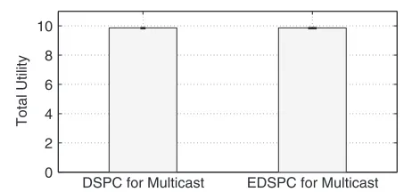
the case shown in Figure 10. As illustrated in Figure 11, both Algorithms 5 and 6 are robust against the initial value variations.

Conclusion

We studied the distributed power control problem of optimizing the system utility as a function of the achiev-able rates in wireless ad hoc networks. Based on the observation that the global optimum lies on the bound-ary of the feasible region for unicast communications, we focused on the equivalent but more structured prob-lem in the form of maximizing the minimum weighted utility. Appealing to EDT, we decomposed the minimum weighted utility maximization problem into subproblems by using penalty multipliers for constraint violations. We then proposed a DSPC algorithm to seek a globally opti-mal solution, where each user stochastically announces its target utility to improve the total system utility via SA. In spite of the nonconvexity of the underlying problem, the DSPC algorithm can guarantee global optimality, but only with a slow convergence rate. Therefore, we proposed an EDSPC to improve the convergence rate with geomet-ric cooling schedule in SA. We then compared DSPC and

DSPC for Multicast EDSPC for Multicast 0

2 4 6 8 10

Total Utility

Figure 11Comparison of average performance (with conﬁdence interval) of DSPC and EDSPC for multicast.

EDSPC with the existing power control algorithms and veriﬁed the optimality and complexity reduction.

Next, we proposed the joint scheduling and power allocation policy for queueing systems by integrating our distributed power control algorithms with the back-pressure algorithm. The stability region was evaluated, which is shown to be strictly greater than the throughput region in the corresponding saturated case. Beyond uni-cast communications, we generalized our power control algorithms to multicast communications by jointly maxi-mizing the minimum rates on bottleneck links in diﬀerent multicast groups. Our DSPC approach guarantees global optimality without the need of channel information, while reducing the computation complexity, in general systems with unicast and multicast communications, and applies to both backlogged and random traﬃc patterns.

Endnotes

a _{We use the terms “user” and “link” interchangeably}

throughout the article.

b_{We use bold symbols (e.g.,}_{p) to denote vectors and}

cal-ligraphic symbols (e.g.,L) to denote sets.

c_{The QoS constraint for each link can be incorporated in}

(2), and the proposed algorithms in the following section can easily be adapted to this case at the cost of added nota-tional complexity.

d_{For some special utility functions}_U

l(·), (2) can be trans-formed into a convex problem [3]. In this article, we focus on the nonconvex case that cannot be transformed to a convex problem by change of variables.

e _{The local optimal solution found by ADP matches the}

globally optimal solution only in one of the cases that are illustrated in Table 2.

f _{By deﬁnition, a function}_f _: _Rn _→ _R_{is quasi-convex,}

if its domaindomf and all its sublevel sets Sc = {x ∈ domf|f(x)≤c}, forc∈R, are convex [26].

g _{A power control algorithm is of standard form, if the}

interference function (the eﬀective interference each link must overcome) is positive, monotonic and scalable in power allocation [27].

h_{The geometric cooling schedule is employed to}

acceler-ate the convergence racceler-ate of DSPC in the simulation. DSPC updates penalty values until they satisfy the threshold-based optimality condition.

i _{Note that the feasible utility region} _F _{deﬁned in}

Section “Power control for unicast communications” is the throughput region, when the utility function is the same as the rate function.

j _{The transmission mode is deﬁned as the transmission}

rate pair within the throughput regionF.

k _{The other existing algorithms have speciﬁcally been}

(14)

Competing interests

The authors declare that they have no competing interests.

Acknowledgements

This study was supported in part by the DoD MURI Project FA9550-09-1-0643 and the AFOSR grants FA9550-10-C-0026 and FA9550-11-C-0006.

Author details

1_{School of ECEE, Arizona State University, Tempe, AZ 85287, USA.}2_Intelligent

Automation, Inc., Rockville, MD 20855, USA.

Received: 15 February 2012 Accepted: 4 July 2012 Published: 24 July 2012

References

1. M Chiang, P Hande, T Lan, CW Tan, Power control in wireless cellular networks. Found. Trends Netw.2(4), 381–553 (2008)

2. D Julian, M Chiang, D O’Neill, S Boyd, Qos and fairness constrained convex optimization of resource allocation for wireless cellular and ad hoc networks. inProc. IEEE INFOCOM,vol. 2 (New York, USA, 2002), pp. 477–486 3. M Chiang, CW Tan, D Palomar, D O’Neill, D Julian, Power control by

geometric programming. IEEE Trans. Wirel. Commun.1(7), 2640–2651 (2007)

4. M Xiao, NB Shroﬀ, EKP Chong, A utility-based power control scheme in wireless cellular systems. IEEE/ACM Trans. Netw.11(2), 210–221 (2003) 5. Z-Q Luo, S Zhang, Dynamic spectrum management: complexity and

duality. IEEE J. Sel. Topics Signal Process.2(1), 57–73 (2008) 6. J Huang, R Berry, M Honig, Distributed interference compensation for

wireless networks. IEEE J. Sel. Areas Commun.24(5), 1074–1084 (2006) 7. P Hande, S Rangan, M Chiang, X Wu, Distributed uplink power control for

optimal SIR assignment in celluar data networks. IEEE/ACM Trans. Netw.

16(6), 1420–1433 (2008)

8. J Papandriopoulos, S Dey, J Evans, Optimal and distributed protocols for cross-layer design of physical and transport layers in MANETs. IEEE/ACM Trans. Netw.16(6), 1392–1405 (2008)

9. J Papandriopoulos, JS Evans, SCALE: a low-complexity distributed protocol for spectrum balancing in multiuser DSL networks. IEEE Trans. Inf. Theory.55(8), 3711–3724 (2009)

10. CU Saraydar, NB Mandayam, DJ Goodman, Eﬃcient power control via pricing in wireless data networks. IEEE Trans. Commun.50(2), 291–303 (2002)

11. T Alpcan, T Basar, R Srikant, E Altman, Wirel. Netw.8(6), 659–670 (2002) 12. Y Xu, T Le-Ngoc, S Panigrahi, Global concave minimization for optimal

spectrum balancing in multi-user DSL networks. IEEE Trans. Signal Process.56(7), 2875–2885 (2008)

13. R Horst, H Tuy,Global Optimization—Deterministic Approaches(Springer, New York, 2006)

14. L Qian, YJ Zhang, J Huang, MAPEL: achieving global optimality for a non-convex power control problem. IEEE Trans. Wirel. Commun.8(3), 1553–1563 (2009)

15. L Qian, YJ Zhang, M Chiang, Globally optimal distributed power control for nonconcave utility maximization. inProc. IEEE GLOBECOM(Miami, USA, 2010), pp. 1–6

16. S Geman, D Geman, Stochastic relaxation, Gibbs distributions, and the Bayesian restoration of images. IEEE Trans. Pattern Anal. Mach. Intell.6(6), 721–741 (1984)

17. Y Chen, M Chen, Extended duality for nonlinear programming. Comput. Optim. Appl.47(1), 33–59 (2010)

18. S Kirkpatrick, CD Gelatt, JMP Vecchi, Optimization by simulated annealing. Science.220(4598), 671–680 (1983)

19. B Hajek, Cooling schedules for optimal annealing. Math. Oper. Res.13(2), 311–329 (1988)

20. L Tassiulas, A Ephremides, Stability properties of constrained queueing systems and scheduling policies for maximum throughput in multihop radio networks. IEEE Trans. Autom. Control.37(12), 1936–1948 (1992) 21. MJ Neely, E Modiano, CE Rohrs, Dynamic power allocation and routing for

time varying wireless networks. IEEE J. Sel. Areas Commun.23(1), 89–103 (2005)

22. H-W Lee, E Modiano, LB Le, Distributed throughput maximization in wireless networks via random power allocation. IEEE Trans. Mob. Comput.

11(4), 577–590 (2011)

23. JE Wieselthier, GD Nguyen, A Ephremides, On construction of energy-eﬃcient broadcast and multicast trees in wireless networks. in Proc. IEEE INFOCOM,vol. 2 (Tel Aviv, Israel, 2000), pp. 585–594 24. K Wang, CF Chiasserini, JG Proakis, RR Rao, Joint scheduling and power

control supporting multicasting in wireless ad hoc networks.4(4), 532–546 (2006). Ad Hoc Netw

25. J Mo, J Walrand, Fair end-to-end window-based congestion control. IEEE/ACM Trans. Netw.8(5), 556–567 (2000)

26. S Boyd, L Vandenberghe,Convex Optimization(Cambridge University Press, Cambridge, UK, 2004)

27. RD Yates, A framework for uplink power control in cellular radio systems. IEEE J. Sel. Areas Commun.13(7), 1341–1347 (1995)

28. X Lin, NB Shroﬀ, R Srikant, On the connection-level stability of congestion-controlled communication networks. IEEE Trans. Inf. Theory.

54(5), 2317–2338 (2008)

29. R Rao, A Ephremides, On the stability of interacting queues in a multiple-access system. IEEE Trans. Inf. Theory.34(5), 918–930 (1988) 30. A ParandehGheibi, M Medard, A Ozdaglar, A Eryilmaz, Information theory

vs. queueing theory for resource allocation in multiple access channels. in Proc. IEEE Pers. Ind. Mob. Radio Commun(Nice, France, 2008), pp. 1–5 31. R Loynes, The stability of a queue with non-interdependent inter-arrival

and service times. Proc. Camb. Philos. Soc.58, 497–520 (1962) 32. L Georgiadis, MJ Neely, L Tassiulas, Resource allocation and cross-layer

control in wireless networks. Found. Trends Netw.1(1), 1–149 (2006) 33. P Chaporkar, S Sarkar, Stable scheduling policies for maximizing

throughput in generalized constrained queueing systems. IEEE Trans. Autom. Control.53(8), 1913–1931 (2008)

34. Y Yi, J Zhang, M Chiang, Delay and eﬀective throughput of wireless scheduling in heavy traﬃc regimes: vacation model for complexity. in Proc. ACM Mobihoc(New York, USA, 2009), pp. 55–64

doi:10.1186/1687-1499-2012-231

Cite this article as:Yanget al.:Distributed stochastic power control in ad hoc networks: a nonconvex optimization case.EURASIP Journal on Wireless Communications and Networking20122012:231.

Submit your manuscript to a

journal and beneﬁ t from:

7Convenient online submission 7Rigorous peer review

7Immediate publication on acceptance 7Open access: articles freely available online 7High visibility within the ﬁ eld

7Retaining the copyright to your article