Rate of convergence of solutions of rational difference equation of second order

DIFFERENCE EQUATION OF SECOND ORDER

Received 13 August 2003 and in revised form 7 October 2003

We investigate the rate of convergence of solutions of some special cases of the equation xn+1=(α+βxn+γxn−1)/(A+Bxn+Cxn−1), n=0, 1,..., with positive parameters and nonnegative initial conditions. We give precise results about the rate of convergence of the solutions that converge to the equilibrium or period-two solution by using Poincar´e’s theorem and an improvement of Perron’s theorem.

1. Introduction and preliminaries

We investigate the rate of convergence of solutions of some special types of the second-order rational difference equation

xn+1= α+βxn+γxn−1

A+Bxn+Cxn−1, n=0, 1,..., (1.1)

where the parametersα,β,γ,A,B, andCare positive real numbers and the initial condi-tionsx−1,x0are arbitrary nonnegative real numbers.

Related nonlinear second-order rational difference equations were investigated in [2, 5,6,7,8,9,10]. The study of these equations is quite challenging and is in rapid devel-opment.

In this paper, we will demonstrate the use of Poincar´e’s theorem and an improvement of Perron’s theorem to determine the precise asymptotics of solutions that converge to the equilibrium.

We will concentrate on three special cases of (1.1), namely, forn=0, 1,...,

xn+1= B xn+

C

xn−1, (1.2)

xn+1= pxn+xn−1

qxn+xn−1, (1.3)

xn+1= pxn+xn−1

q+xn−1 , (1.4)

where all the parameters are assumed to be positive and the initial conditionsx−1,x0are arbitrary positive real numbers.

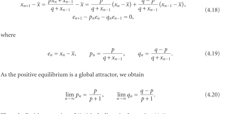
In [7], the second author and Ladas obtained both local and global stability results for (1.2), (1.3), and (1.4) and found the region in the space of parameters where the equilib-rium solution is globally asymptotically stable. In this paper, we will precisely determine the rate of convergence of all solutions in this region by using Poincar´e’s theorem and an improvement of Perron’s theorem.

We will show that the asymptotics of solutions that converge to the equilibrium de-pends on the character of the roots of the characteristic equation of the linearized equa-tion evaluated at the equilibrium. The results on asymptotics of (1.2), (1.3), and (1.4) will show all the complexity of the asymptotics of the general equation (1.1).

Here we give some necessary definitions and results that we will use later.

LetIbe an interval of real numbers and letf ∈C1_{[I×I,I]. Let ¯x∈Ibe an equilibrium} point of the difference equation

xn+1= fxn,xn−1

, n=0, 1,..., (1.5)

that is, ¯x= f( ¯x, ¯x). Let

s=∂ f

∂u( ¯x, ¯x), t= ∂ f

∂v( ¯x, ¯x) (1.6)

denote the partial derivatives of f(u,v) evaluated at an equilibrium ¯xof (1.5). Then the equation

yn+1=syn+tyn−1, n=0, 1,..., (1.7)

is called thelinearized equationassociated with (1.5) about the equilibrium point ¯x.

Theorem1.1 (linearized stability). (a)If both roots of the quadratic equation

λ2_{−sλ−t=0 (1.8)}

lie in the open unit disk|λ|<1, then the equilibrium x¯ of (1.5) is locally asymptotically stable.

(b)If at least one of the roots of (1.8) has an absolute value greater than one, then the equilibriumx¯of (1.5) is unstable.

(c)A necessary and sufficient condition for both roots of (1.8) to lie in the open unit disk |λ|<1is

|s|<1−t <2. (1.9)

In this case, the locally asymptotically stable equilibriumx¯is also called a sink.

(d)A necessary and sufficient condition for both roots of (1.8) to have absolute values greater than one is

|t|>1, |s|<|1−t|. (1.10)

(e)A necessary and sufficient condition for one root of (1.8) to have an absolute value greater than one and for the other to have an absolute value less than one is

s2_{+ 4t >0, |s|>|1−t|. (1.11)}

In this case, the unstable equilibriumx¯is called a saddle point.

The set of points whose orbits converge to an attracting equilibrium point or, periodic point is called the “basin of attraction,” see [1, page 128].

Definition 1.2. LetTbe a map onR2_{and letpbe an equilibrium point or a periodic point} forT. Thebasin of attractionofp, denoted byᏮp, is the set of pointsx∈R2_{such that} |Tk_(x)−Tk_{(p)| →0, ask→ ∞, that is,}

Ꮾp=x∈R2_:Tk_(x)−Tk_{(p)−→0, ask−→ ∞, (1.12)}

where| · |denotes any norm inR2_.

We now give the definitions of positive and negative semicycles of a solution of (1.5) relative to an equilibrium point ¯x.

A positive semicycle of a solution{xn} of (1.5) consists of a “string” of terms{xl, xl+1,...,xm}, all greater than or equal to the equilibriumx, withl≥ −1 andm≤ ∞and such that eitherl= −1 orl >−1,xl−1< x, and eitherm= ∞orm <∞,xm+1< x.A neg-ative semicycleof a solution{xn}of (1.5) consists of a string of terms{xl,xl+1,...,xm}, all less than the equilibriumx, withl≥ −1 andm≤ ∞and such that eitherl= −1 orl > −1,xl−1≥x, and eitherm= ∞orm <∞,xm+1≥x.

The next theorem is a slight modification of the result obtained in [7,9].

Theorem1.3. Assume that

f : [0,∞)×[0,∞)−→[0,∞) (1.13)

is a continuous function satisfying the following properties:

(a)there existLandU,0< L < U, such that

f(L,L)≥L, f(U,U)≤U, (1.14)

and f(x,y)is nondecreasing inxandyin[L,U]; (b)the equation

f(x,x)=x (1.15)

has a unique positive solution in[L,U].

Proof. Set

m0=L, M0=U, (1.16)

and fori=1, 2,..., set

Mi=f

Mi−1,Mi−1

, mi=f

mi−1,mi−1

. (1.17)

Now observe that for eachi≥0,

m0≤m1≤ ··· ≤mi≤ ··· ≤Mi≤ ··· ≤M1≤M0,

mi≤xk≤Mi fork≥2i+ 1. (1.18)

Now the proof follows as the proof of [7, Theorem 1.4.8].

The next two theorems give precise information about the asymptotics of linear non-autonomous difference equations. Consider the scalarkth-order linear difference equa-tion

x(n+k) +p1(n)x(n+k−1) +···+pk(n)x(n)=0, (1.19)

wherekis a positive integer andpi:Z+_{→Cfori=1,...,k. Assume that}

qi=lim

k→∞pi(n), i=1,...,k, (1.20)

exist inC. Consider thelimiting equationof (1.19):

x(n+k) +q1x(n+k−1) +···+qkx(n)=0. (1.21)

Then the following results describe the asymptotics of solutions of (1.19). See [4,3, 11].

Theorem1.4 (Poincar´e’s theorem). Consider (1.19) subject to condition (1.20). Letλ1,..., λkbe the roots of the characteristic equation

λk+q1λk−1+···+qk=0 (1.22)

of the limiting equation (1.21), and suppose that

_{λi=λj fori=j. (1.23)}

Ifx(n)is a solution of (1.19), then eitherx(n)=0for all largenor there exists an index j∈ {1,...,k}such that

lim n→∞

x(n+ 1)

The related results were obtained by Perron, and one of Perron’s results was improved by Pituk, see [11].

Theorem1.5. Suppose that (1.20) holds. Ifx(n)is a solution of (1.19), then eitherx(n)=0 eventually or

lim sup n→∞

_xj(n)1/n₌

λj, (1.25)

whereλ1,...,λkare the (not necessarily distinct) roots of the characteristic equation (1.22).

2. Rate of convergence ofxn+1=(B/xn) + (C/xn−1)

Equation (1.2) has a unique equilibrium pointx=√B+C.The linearized equation asso-ciated with (1.2) aboutxis

zn+1+ B B+Czn+

C

B+Czn−1=0, n=0, 1,.... (2.1) This equation was considered in [7], where the method of full limiting sequences was used to prove that the equilibrium is globally asymptotically stable for all values of param-etersBandC. Here, we want to establish the rate of this convergence. The characteristic equation

λ2+ B B+Cλ+

C

B+C =0, n=0, 1,..., (2.2)

that corresponds to (2.1) has roots

λ±=−B±

B2_−4C(B+C)

2(B+C) . (2.3)

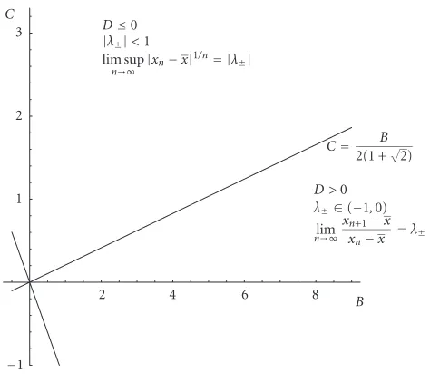
Theorem 2.1. All solutions of (1.2) which are eventually different from the equilibrium satisfy the following.

(i)If the condition

C < B

21 +√2 (2.4)

holds, then

lim n→∞

xn+1−x

xn−x =λ+ or nlim→∞

xn+1−x

xn−x =λ−, (2.5)

whereλ±are the real roots given by (2.3).

In particular, all solutions of (1.2) oscillate. (ii)If the condition

C= B

holds, then

Since the equilibrium is a global attractor, we obtain

lim

Thus, the limiting equation of (1.2) is the linearized equation (2.1) whose characteristic equation is (2.2). The discriminant of this equation is given by

D=B2_{−4C(B+C)=B−2C(B+C) B+ 2C(B+C) . (2.14)}

Conditions (2.4), (2.6), and (2.8) are the conditions forD >0,D=0, andD <0, respec-tively.

Now, statement (i) follows as an immediate consequence of Poincar´e’s theorem and statements (ii) and (iii) follow as the consequences ofTheorem 1.5. Finally, the statement on oscillatory solutions follows from the asymptotic estimate (2.5) and the fact that in

−1 1 2 3

C

2 4 6 8

B D≤0

|λ±|<1 lim sup

n→∞ |xn−x| 1/n_{= |λ±|}

C=_{2(1 +}B√ 2)

D >0

λ±∈(−1,0) lim

n→∞ xn+1−x

xn−x =λ±

Figure 2.1. Regions for the different asymptotic behavior of solutions of (1.2).

Figure 2.1visualizes the regions for the different asymptotic behavior of solutions of (1.2).

3. Rate of convergence ofxn+1=(pxn+xn−1)/(qxn+xn−1)

Equation (1.3) was studied in detail in [7,10], where we have found the region of param-eters for which the equilibrium is globally asymptotically stable and the region where the equation has a unique period-two solution which is locally asymptotically stable.

3.1. Rate of convergence of the equilibrium. Equation (1.3) has a unique equilibrium point

x= p+ 1

q+ 1. (3.1)

To avoid the trivial case, we assume thatp=q.

The linearized equation associated with (1.3) aboutxis

zn+1− p−q

(p+ 1)(q+ 1)zn+

p−q

(p+ 1)(q+ 1)zn−1=0, n=0, 1,.... (3.2)

The characteristic equation

λ2₋ p−q (p+ 1)(q+ 1)λ+

p−q

has the roots

λ±=

p−q±(q−p)(4pq+ 3p+ 5q+ 4)

2(p+ 1)(q+ 1) . (3.4)

This equation was considered in detail in [7,10], where it was proved that the equilib-rium is globally asymptotically stable for values of parameterspandqthat satisfy

p < q <3p+ 1

1−p (3.5)

or

p−1

p+ 3< q < p. (3.6)

Here, we want to establish the rate of convergence.

Theorem 3.1. All solutions of (1.3) which are eventually different from the equilibrium satisfy the following.

(i)If condition (3.5) holds, then (2.5) follows, whereλ±are given by (3.4).

(ii)If condition (3.6) holds, then

lim sup

As the equilibrium is a global attractor, we obtain

lim

Thus, the limiting equation of (1.3) is the linearized equation (3.2).

Now, statement (i) follows as an immediate consequence of Poincar´e’s theorem and

−1

Figure 3.1. Regions for the asymptotic behavior of solutions of (1.3).

Figure 3.1visualizes the regions for the different asymptotic behavior of solutions of (1.3).

3.2. Rate of convergence of period-two solutions. Assume that

q >1 + 3p+pq, (3.12)

The following lemma is now a direct consequence of (3.14).

Lemma3.2. Assume that condition (3.12) holds. Let{yn}∞

n=−1be a solution of (1.3). Then the following statements are true.

(iii)Every solution{yn}∞n=−1of (1.3) with initial conditions that satisfy

y−1>Ψ, y0<Φ or y−1<Φ, y0>Ψ (3.15)

oscillates with semicycles of length one. More precisely, such a solution oscillates about the strip[Φ,Ψ]with semicycles of length one.

Proof. (i) The proof follows from

yN+1−Ψ>(q−p)Φ yN−1−Ψ yN−1+qyN

(Ψ+qΦ). (3.16)

(ii) Similarly, the proof is an immediate consequence of

yN+1−Φ<(q−p)Ψ yN−1−Φ yN−1+qyN

(Φ+qΨ). (3.17)

(iii) The proof follows from (i) and (ii).

Now, we will combine our results for semicycles to identify solutions which converge to the period-two solution.

Theorem3.3. Assume that condition (3.12) holds. Then every solution of (1.3) with initial conditions

y−1>1, y0< p

q (3.18)

or

y−1< p

q, y0>1 (3.19)

converges to the period-two solution...,Φ,Ψ,Φ,Ψ,...,whereΦ<Ψare the roots of

t2−(1−p)t+ p(1−p)

q−1 =0. (3.20)

Proof. We will prove the statements in the case (3.18). The proof of the second case is similar.

It is known that forq > p, which holds in view of (3.12), the interval [p/q, 1] is an invariant and attracting interval for (1.3), and thatyn∈[p/q, 1],n≥1, for every solution {yn}of (1.3), see [7,10]. In particular,p/q <Φ<Ψ<1. ThenLemma 3.2implies that

y2k+1>Ψ, y2k+2<Φ, k=0, 1,.... (3.21)

Further, by using the identity

yn+1−yn−1= yn−1

1−yn−1

+qynp/q−yn−1

yn−1+qyn

we obtain

By using induction, we obtain

···< y5< y3< y1, y2< y4< y6<···. (3.25)

In view of the uniqueness of the prime period-two solution, we have

L=Ψ, l=Φ, (3.28)

which completes the proof of the theorem.

The last theorem gives us information about the basin of attraction of the prime period-two solutions, which we denote byB2. We have shown that

Now, we will combine our results for convergence to period-two solution of (1.3) to obtain the rate of convergence.

By using identities (3.14) andTheorem 3.3, we obtain

where

Bk=(Φ+qΨ)y2k−2+qy2k−1

. (3.33)

By using (3.32), identity (3.30) implies

y2k+2−Φ=(q−p)Φ

Thus, the limiting equation of (3.36) is

ek+1−(1 + 2p+pq)(q−1)(1−p) +p(q−p) (1−p)(q−p)(q−1) ek+

p

(q−1)(1−p)ek−1=0. (3.39)

The characteristic equation of (3.39) is

λ2₋(1 + 2p+pq)(q−1)(1−p) +p(q−p) (1−p)(q−p)(q−1) λ+

p

(q−1)(1−p)=0. (3.40)

The discriminant of (3.40) is

If condition (3.12) holds, thenDcan be greater or less than zero. By using (3.32), we obtain

ek+1−akek+bkek−1=0, k=0, 1,..., (3.42)

Thus, the limiting equation of (3.42) is (3.39). Using Poincar´e’s theorem andTheorem 1.5, we obtain the following result which describes the precise asymptotics of convergence to a period-two solution.

Theorem3.4. Assume that condition (3.13) holds. Then every solution{xn}∞

n=−1of (1.3), which is eventually different from a period-two solution, that converges to a period-two so-lution satisfies one of the following two asymptotic relations:

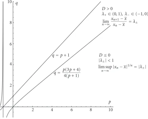
4. Rate of convergence ofxn+1=(pxn+xn−1)/(q+xn−1)

Equation (1.4) was investigated in detail in [7,9]. Here, we assume that p and q are positive parameters.

Equation (1.4) has two equilibrium pointsx=0 andx=p+ 1−qifp+ 1> q. The linearized equation of (1.4) at the zero equilibrium is

zn+1−p

The solutions of (4.2) are

λ±=

p±p2_{+ 4q}

2q . (4.3)

The linearized equation of (1.4) at the positive equilibriumxis

zn+1− p

The solutions of (4.5) are

λ±=₂₍ 1

p+ 1)

p±4q(p+ 1)−p(3p+ 4) . (4.6)

Now, we give two results that describe precisely the asymptotics of the solutions that converge to either zero or the positive equilibrium.

Theorem4.1. Assume thatp+ 1≤q. Then the zero equilibrium of (1.4) is globally asymp-totically stable and

for every solutionxnof (1.4) which is eventually different from the zero equilibrium. Here, λ±are given by (4.6).

Proof. Global asymptotic stability was established in [7,9]. Now, we can represent (1.4) in the form

xn+1=pxn +xn−1

where

an= p

q+xn−1, bn= 1

q+xn−1, (4.9)

with

lim n→∞an=

p

q, nlim→∞bn=

1

q. (4.10)

Thus, the limiting equation is exactly the linearized equation (4.1), and an application of

Poincar´e’s theorem completes the proof of the theorem.

Now, we assume thatp+ 1> q.

Theorem4.2. Assume that p+ 1> q andx−1+x0>0. Then the positive equilibrium of (1.4) is globally asymptotically stable and the solutions exhibit one of the following two types of asymptotic behavior.

(i)Suppose that the condition

q > p(3p+ 4)

4(p+ 1) (4.11)

is satisfied. Then every solution{xn}of (1.4) which is eventually different from the equilibrium satisfies one of the following two limit relations:

lim n→∞

xn+1−x

xn−x =λ+ or nlim→∞

xn+1−x

xn−x =λ−, (4.12)

whereλ±are the real roots given by (4.6).

Ifp=q, then every solution{xn}of (1.4) which is eventually different from the equilibrium satisfies one of the following two limit relations:

lim n→∞

xn+1−x

xn−x =λ±, (4.13)

whereλ±is either0orp/(p+ 1).

(ii)Suppose that the condition

q≤ p(3p+ 4)

4(p+ 1) (4.14)

is satisfied. Then every solution{xn}of (1.4) which is eventually different from the equilibrium satisfies

lim sup n→∞

_xn−x1/n₌

λ±, (4.15)

Proof. The proof of global asymptotic stability was given in [7,9]. Here, we want to cor-rect the proof in the case wherep < q. As we have shown in [7,9], in this case, the interval (0, 1) is invariant and attracting in the sense that every positive solution eventually enters and remains in the interval (0, 1). Now, in the interval (0, 1), the function

f(u,v)= pu+v

q+v (4.16)

is increasing in both arguments and it has a unique equilibrium. Now, we check condi-tion (a) ofTheorem 1.3. We try to determineL,U, 0< L < p+ 1−q < U, that satisfy the (1.4) converges to the positive equilibrium, and since this equilibrium is locally asymp-totically stable, it is also globally asympasymp-totically stable.

Now, we will establish results on the rate of convergence to the positive equilibrium. We have

As the positive equilibrium is a global attractor, we obtain

lim

Thus, the limiting equation of (1.4) is the linearized equation (4.4).

Now, statement (i) follows as an immediate consequence of Poincar´e’s theorem and statement (ii) follows as a consequence ofTheorem 1.5. Conditions (4.11) and (4.14) are actually conditions for the characteristic equation (4.5) to have two real distinct roots and

to have double or complex conjugate roots, respectively.

2 4 6 8 10

p

2 4 6 8 10 _q

q=p(3p+ 4) 4(p+ 1)

q=p+ 1 D≤0 |λ±|<1 lim sup

n→∞ |xn−x| 1/n_{= |λ±|} D >0

λ+∈(0,1), λ−∈(−1,0)

lim

n→∞ xn+1−x

xn−x =λ±

Figure 4.1. Regions for the asymptotic behavior of solutions of (1.4).

5. Rate of convergence of (1.1)

Consider (1.1) where the parametersα,β,γ,A,B, andCare nonnegative real numbers and the initial conditionsx−1andx−2are arbitrary nonnegative real numbers such that

A+Bxn+Cxn−1>0 ∀n≥0. (5.1)

The equilibrium point of (1.1) is

¯

x= α+ ¯x(β+γ)

A+ ¯x(B+C). (5.2)

Then we have

xn+1−x¯=anxn−x¯+bnxn−1−x¯, n=0, 1,..., (5.3)

where

an= βA−αB+x(βC−γB) A+Bxn+Cxn−1

A+ ¯x(B+C),

bn= γA−αC+x(γB−βC) A+Bxn+Cxn−1

A+ ¯x(B+C).

(5.4)

Setxn−x¯=en.Then (5.3) becomes

where

The limiting equation associated with (5.5) is

en+1−βA−αB+x(βC−γB) A+ ¯x(B+C)2 en−

γA−αC+x(γB−βC)

A+ ¯x(B+C)2 en−1=0, n=0, 1,.... (5.7)

The characteristic equation of (5.7) is

λ2₋βA−αB+x(βC−γB)

which is exactly the characteristic equation of the linearized equation of (1.1) evaluated at the positive equilibrium ¯x.

Using Poincar´e’s theorem andTheorem 1.5, we obtain the following result which de-scribes the precise asymptotic behavior of solutions converging to the positive equilib-rium.

Theorem5.1. (i)If the discriminant of (5.8) is positive, then every solution{xn}of (1.1) which is eventually different from the equilibrium satisfies one of the two limit relations in (4.12), whereλ±are the real roots of (5.8).

In particular, (1.1) has all oscillatory solutions if both rootsλ±are negative, and has all

solutions nonoscillatory if both rootsλ±are positive.

(ii)If the discriminant of (5.8) is nonpositive, then every solution{xn}of (1.1) which is eventually different from the equilibrium satisfies (3.7), whereλ±are the complex roots of

(5.8).

Acknowledgments

The authors are grateful to the referees for numerous comments that improved the quality of the paper. The first author is on research leave from the Department of Mathematics, University of Sarajevo, Sarajevo, Bosnia and Herzegovina.

References

[1] K. T. Alligood, T. D. Sauer, and J. A. Yorke,Chaos. An Introduction to Dynamical Systems, Text-books in Mathematical Sciences, Springer-Verlag, New York, 1997.

[2] H. El-Metwally, E. A. Grove, and G. Ladas,A global convergence result with applications to peri-odic solutions, J. Math. Anal. Appl.245(2000), no. 1, 161–170.

[3] S. N. Elaydi,An Introduction to Difference Equations, 2nd ed., Undergraduate Texts in Mathe-matics, Springer-Verlag, New York, 1999.

[4] ,Recent developments in the asymptotics of difference equations, New Developments in Difference Equations and Applications (Taipei, 1997), Gordon and Breach, Amsterdam, 1999, pp. 161–181.

[5] C. H. Gibbons, M. R. S. Kulenovi´c, and G. Ladas, On the recursive sequence xn+1=(α+

[6] V. L. Koci´c and G. Ladas,Global Behavior of Nonlinear Difference Equations of Higher Order with Applications, Mathematics and Its Applications, vol. 256, Kluwer Academic Publishers, Dordrecht, 1993.

[7] M. R. S. Kulenovi´c and G. Ladas,Dynamics of Second Order Rational Difference Equations, Open Problems and Conjectures, Chapman & Hall/CRC, Florida, 2002.

[8] M. R. S. Kulenovi´c, G. Ladas, and N. R. Prokup,On the recursive sequence xn+1=(αxn+

βxn−1)/(A+xn), J. Differ. Equations Appl.6(2000), no. 5, 563–576.

[9] ,A rational difference equation, Comput. Math. Appl.41(2001), no. 5-6, 671–678. [10] M. R. S. Kulenovi´c, G. Ladas, and W. S. Sizer, On the recursive sequence xn+1=(αxn+

βxn−1)/(γxn+δxn−1), Math. Sci. Res. Hot-Line2(1998), no. 5, 1–16.

[11] M. Pituk,More on Poincar´e’s and Perron’s theorems for difference equations, J. Difference Equ.

Appl.8(2002), no. 3, 201–216.

S. Kalabuˇsi´c: Department of Mathematics, University of Rhode Island, Kingston, RI 02881-0816, USA

E-mail address:[email protected]

M. R. S. Kulenovi´c: Department of Mathematics, University of Rhode Island, Kingston, RI 02881-0816, USA