Minimum Delay POIs Coverage in mobile wireless sensor networks

(1)

R E S E A R C H

Open Access

Minimum-Delay POIs Coverage in mobile

wireless sensor networks

Wenping Chen

*

, Si Chen and Deying Li

Abstract

In some mobile wireless sensor network applications, it is not necessary to monitor the entire field all the time, and only a number of critical points or points of interest (POIs) need to be monitored periodically. In this paper, we address theminimum-delay POIs coverageinmobile wireless sensor networksproblem with cost restriction, which is how to schedule the limited number of mobile sensors monitoring to minimize the service delay of POIs. We study two scenarios of the problem. In the first scenario, the start positions of mobile sensors are determined in advance, we propose theSSRalgorithm to address this problem. In the second scenario, without pre-defined start positions, we propose two algorithms, theTSP-Sand theSSNOR. By the comprehensive simulations, we evaluate the performance of the proposed algorithms. The simulation results show the efficiency of our algorithms.

Keywords: Sweep coverage; POIs; Mobile sensor; TSP

1 Introduction

Wireless sensor networks(WSNs)have been widely stud-ied in recent years. Coverage is one of the most important issues in WSNs. There have been a great number of works on area coverage, target coverage and barrier cover-age. Most of them require the targets or monitoring area is covered continuously. However, in some applications, such as patrol inspection, only some critical points are needed to be detected periodically. Employing continuous coverage in such application is undoubtedly wasteful.

To satisfy the demands of the above applications with low system cost, another type of coverage called sweep coverage is proposed [1]. The sweep coverage has been applied to practical application, such as GreenOrbs [1], which is a sustainable and large-scale wireless sensor network system in the forest. GreenOrbs provide all-year-round ecological surveillance in the forest in Tianmu Mountain, collecting various sensory data, such as tem-perature, humidity, illumination, and content of carbon dioxide. In sweep coverage, a set of Points of Interests (POIs) in the monitoring area are periodically detected instead of being continuously monitored. To achieve sweep coverage, a downsized number of mobile sensors are employed to sweep the POIs at regular intervals.

*Correspondence: chenwenping@ruc.edu.cn

School of Information, Renmin University of China, Beijing, China

There have been some efforts on the sweep coverage problem [1,2]. These works focus on how to schedule min-imum number of mobile sensors to achieve the sweep cov-erage within specified sweep period. The existing works assumed that they have enough mobile sensors. However, in real applications, there may have been restrictions on the number of mobile sensors due to the system cost.

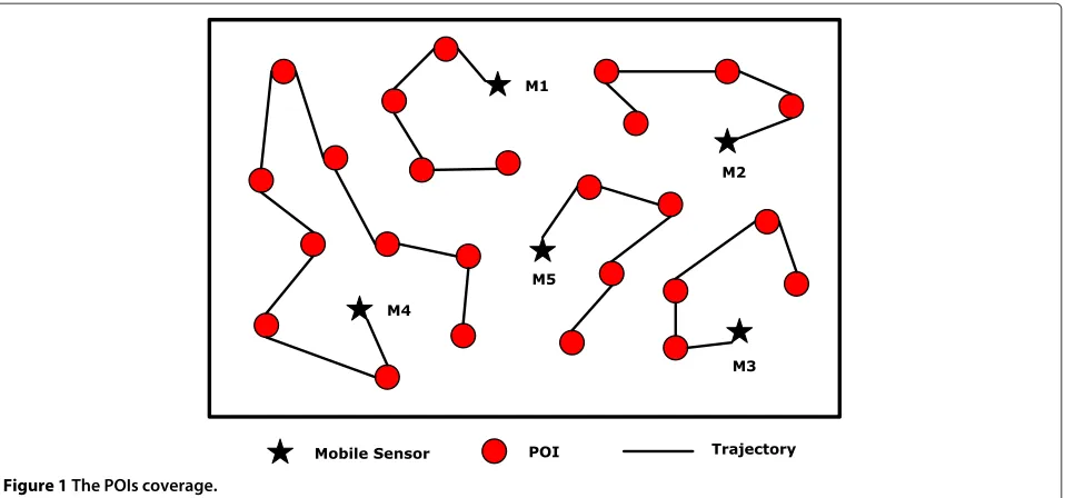
In this paper, we investigate POI coverage under the restriction on the number of mobile sensors. We address how to schedule the mobile sensors to minimize the sweep delay of POIs. As shown in Figure 1, there are five mobile sensors in the area. Each mobile sensor scans specific POIs in its trajectory, respectively. The delay of the sweep is defined as the time interval from sensors starting to sweep to all the sensors finishing their mon-itoring task. Suppose the moving speed of each mobile sensor is the same; since M4 has the longest trajectory,

the delay of sweep is decided by M4 which is several

times longer than that ofM1,M2,M3, andM5. We study two scenarios of the problem. In the first scenario, the energy of sensors may not be enough to sustain for a long time, such that the sensors must be recharged periodi-cally. Thus, the start positions of mobile sensors located at the recharging places are determined. We present a greedy-based algorithm namedSSR. For each mobile sen-sor’s determined start position, we always choose the POI that can minimize the length difference between

(2)

Figure 1The POIs coverage.

the maximal and minimal trajectories of mobile sen-sors. The procedure continues until all the POIs have been added to the trajectories of mobile sensors. In the second scenario, the energy of sensor is enough to sus-tain for a long time, such that the sensors need not return back frequently. Compared with the long sweep-ing time, the time that the mobile sensor moves from start position to the the first POI to be swept can be ignored. We propose two algorithms. One is construct-ing a travelconstruct-ing salesman problem (TSP) ring using the

polynomial-time approximation scheme (PTAS) for the

TSP [3], then divide the ring into k trajectories and let every mobile sensor move along with a trajectory, respec-tively. The second algorithm is derived from the SSR algorithm.

The rest of this paper is organized as follows: Section 2 reviews the existing works. In Section 3, we introduce

the network model and the definition ofMinimum-Delay

POIs Coverage in mobile wireless sensor networks prob-lem. In Section 4, we propose the Stretched Searching SSR algorithm for the Minimum-Delay POIs Coverage problem with restriction on start positions of mobile

sensors. The TSP-S algorithm and the SSNOR

algo-rithm are presented for the the Minimum-Delay POIs Coverage problem without restriction on start positions of mobile sensors in Section 5. We evaluate the per-formance of our algorithms through extensive simula-tions in Section 6. Finally, we conclude the paper in Section 7.

2 Related work

The coverage problem is one of the fundamental issues in wireless sensor networks, evidenced by many works

contribute to this field in recent years. It can be classified into three categories: full coverage, barrier coverage, and sweep coverage.

Many efforts have been made on full coverage prob-lem (including point coverage [4-8], area coverage [9-18]), and barrier coverage problem [19-26]. Full coverage and barrier coverage often require that target or area is cov-ered all the time. To achieve full coverage or barrier coverage, a majority of works studied the static coverage under the requirement of continuous coverage. Although it can achieve the best coverage, the system cost is pro-hibitive. To improve the coverage quality efficiently, a type of mixed network infrastructure called hybrid network is adopted in some applications, which is composed of mobile sensors as well as static sensors [27-30]. Wang et al. studied the optimized movement of mobile sensors

to provide k-coverage in both mobile sensor networks

and hybrid sensor networks [27]. They also presented a distributed relocation algorithm, such that each mobile sensor can achieve optimal relocation with the local information.

(3)

Du et al. [2] proposed two algorithms for different situa-tions. In the first algorithm, they gradually deploy mobile sensors and schedule the mobile sensors to move on the same trajectory in each period. In the second algorithm, named OSWEEP algorithm, the mobile sensors are not required to follow the same trajectory in each period, all the mobile sensors are scheduled to move along the TSP ring which consists of POIs towards the same direction. The OSWEEP algorithm has better performance than CSWEEP.

Both of the works assumed that they can obtain enough mobile sensors. However, in many practical applications, due to high energy consumptions and resource con-straints, there may not be enough mobile sensors to accomplish monitoring.

In this paper, we consider the situation that the number of mobile sensors is given. We discuss two scenarios for the problem: (1) the start positions of mobile sensors are determined in advance; (2) the start positions of mobile sensors are not determined, and we ignore the time that mobile sensor moves from start position to the first POI to be swept.

3 Minimum-Delay POIs Coverage in mobile wireless sensor networks problem

3.1 Network model

Suppose there arek given mobile sensors to monitor m

POIs deployed in a region R. Each POI has a globally

unique ID and a fixed position. We denote the set of mobile sensors asS = {s1,. . .,sk} and the set of POIs asP = {p1,. . .,pm}. Let d(pi,pj) be the Euclidean dis-tance between pointspiandpj. There are two scenarios. In the first one, all mobile sensors start from the determined positions to scan specific POIs along different trajecto-ries and go back to the start position to recharge after a period. In the second one, the mobile sensors have enough energy to sweep POIs for quite a long time, therefore, the distance from recharging place to start position of each mobile sensor is ignored. We assume that all the mobile sensors move at a constant speedvin the region. In fact, if the moving speed of mobile sensor is not the same when generating trajectory for each mobile sensor, we will take its speed as a ratio to compute the distance of the trajectory. We also assume the sensing range of all mobile sensors is very small such that the POIs can be covered only when the mobile sensors pass the position of the POIs.

In this paper, we study the minimum-delay POIs cov-erage in mobile wireless sensor networks. We aim to schedulekmobile sensors to scan those POIs such that the delay of the mobile wireless sensors network(MWSN)is minimized and each POI can be scanned exactly one time in a period.

3.2 Problem definition

Before formalizing the Minimum-Delay POIs Coverage in mobile wireless sensor networks problem, we first intro-duce a few of definitions as follows:

Definition 1. POIs Coverage (PC): If all POIs are swept by some mobile sensors, we call it POIs Coverage.

Definition 2. The Delay of POIs Coverage: The delay of POIs Coverage is the time interval from the mobile sensors starting to sweep to all POIs having been swept.

Definition 3. Minimum-Delay POIs Coverage in mobile wireless sensor networks problem: Given k mobile sensors and the deployments of m POIs, the Minimum-Delay POIs Coverage problem is to schedule k mobile sensors to scan POIs along different trajectories such that the delay of the POIs coverage is minimized.

If there is no restriction on the start positions of mobile sensors, given the deployment of POIs, an undirected complete graphG=(V,E,W)is derived from the mobile wireless sensor network, where V is the set of all POIs. For any two POIspi,pj, there is an edge betweenpi and

pj (i.e., (pi,pj) ∈ E), and w(e) = d(pi,pj). If there is restriction on start positions of mobile sensor, given the deployment of POIs, an undirected weight graphGstart=

(V,Vstart,Estart,W) is derived, whereV is the set of all POIs andVstartis the set of start positions of mobile sen-sors. For any two POIspi,pj, there is an edge betweenpi andpj (i.e.,(pi,pj) ∈ Estart), and w((pi,pj)) = d(pi,pj); for any start position of mobile sensor si and any POI

pj, there must be an edge (si,pj)betweensi andpj (i.e., (si,pj)∈Estart), andw((si,pj))=d(si,pj).

Based on the given Euclidean distance between any two points, finding a coverage scheme for the Minimum-Delay POIs Coverage problem is equivalent to finding a set of trajectories which can pass by all the POIs.

Apparently, the Minimum-Delay POIs Coverage prob-lem can be transformed to the probprob-lem of minimizing the maximal trajectory of mobile sensors: givenkmobile sensors, find a set ofktrajectories to pass all POIs such

that the maximum length among all k trajectories is

minimized.

It is easy to know that the problem with no restriction on the start positions of mobile sensors is NP-hard. This

is because whenk = 1, this problem becomes the

mini-mum length Hamilton Path problem which is well known NP-hard.

4 Algorithm for the Minimum-Delay POIs Coverage with restriction

(4)

of mobile sensors, and propose an algorithm for the prob-lem. To minimize the network delay which is decided by the longest monitoring period among all the mobile sen-sors, we aim to make the sweeping time of each mobile sensor be close to each other.

We first give the following definitions:

Definition 4. Max-min difference for a set of k trajec-tories (2MDkT): Given k trajectories, max-min difference is the length difference between the longest trajectory and the shortest trajectory.

Definition 5. Minimum max-min trajectory schedule: Among the feasible monitoring schedules of k mobile sen-sors, each of which can be represented as a set of the k mobile sensors’ trajectories, minimum max-min trajectory schedule is the one with minimum 2MDkT.

It is easy to know that the Minimum-Delay POIs Cover-age problem is equivalent to the minimum max-min tra-jectory schedule problem. In this section, we propose an effective algorithm, the SSR algorithm for the Minimum-Delay POIs Coverage problem with the restriction on the start positions of mobile sensors.

The main idea of the SSR algorithm is as follows: in every step, we always choose the pair of POI and trajectory such that the 2MDkT of the current MWSN is minimized. Before introducing the SSR algorithm, we give some notations used in the algorithm.

We denote C as the current selected trajectories for mobile sensors. C= {c1,c2,. . .,ck},ci is the ith mobile

sensor’s trajectory. Initially, we may set C= ∅. We

use T to represent the set of POIs which have not

been covered by C. There are k mobile sensors and

n POIs in the region. The input of the algorithm is

Gstart=(V,Vstart,Estart,W). The output of the algorithm is a set C= {c1,c2,. . .,ck} of trajectories which con-tains all vertices in V and Vstart. For the convenience

to describe the algorithm, we let L denote 2MDkT,

Lmin denote the current minimal L in the MWSN.

In the following, we present the SSR algorithm in details.

(1) SetC= ∅and set all POIs to beuncovered. (2) Select the shortest edgees_tinG where s is the start

position of a mobile sensor andt is a POI. Then add t to the trajectory of mobile sensors. Set t to be covered.

(3) As for thePOI i which has not been covered, we tentatively add thePOI to the trajectory of every mobile sensorj(j=[1,. . .,k])and compute theLj_i

respectively.Lj_iis the 2MDkT, that if the POIi is added to the the trajectory of mobile sensorj. Thus, Li= {L1i,L2i,. . .,Lki}.

(4) SetLcur= {L1,L2,. . .,Lm}, wherem is the number of uncovered POIs. Find the minimal element Lj_iinLcurand add the POIi to the trajectory of

mobile sensorj. Then set the POI i to be covered. (5) Repeat steps (3) to (4) until the trajectories inC

contain all vertexes ofV.

(6) Check the trajectory of each mobile sensor, if the trajectory intersects with other trajectories and the distance from start position to the point of intersection is the same, there will be collision between mobile sensors. Adjust the depart time of one of the mobile sensors slightly to avoid collision.

The pseudocode of the SSR algorithm is presented in Algorithm 1.

(5)

a

b

c

d

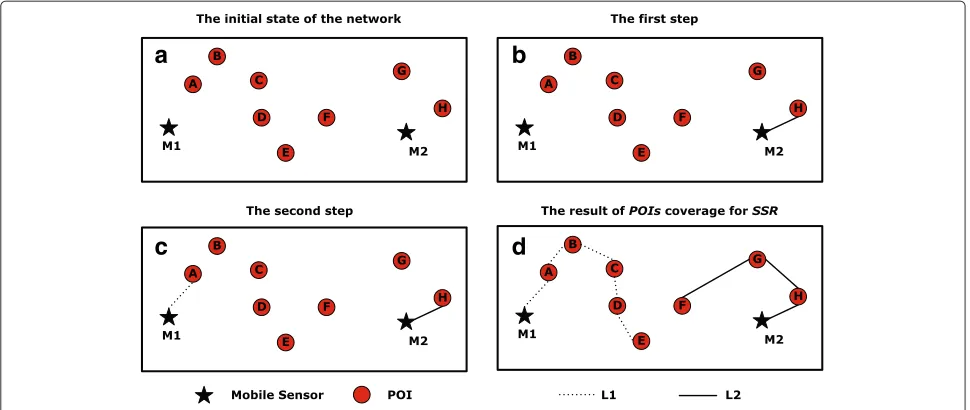
Figure 2An example of POIs coverage for SSR.(a)There are two mobile sensors and eight POIs in the region.(b)POIHis added to the trajectory ofM2.(c)POIAis added to the trajectory ofM1.(d)The trajectories ofM1 andM2 is constructed after the rest of the POIs are added one by one.

To better describe the SSR algorithm, we give an exam-ple as follows: in Figure 2a, there are two mobile sensors and eight POIs in the rectangle region. The weight of edge, which is the distance between two points in the area is illustrated in Table 1. We setv = 100 m/min for each mobile sensor. Firstly, as M2H is the smallest edge

connected to the mobile sensors, we add POI H to the

trajectory of mobile sensor M2 as shown in Figure 2b. Secondly, for each of the rest uncovered POIs, we tenta-tively add these seven POIs to the trajectories of mobile

sensorsM1 andM2. Meanwhile, we compute the 2MDkT

in the current mobile sensor network after tentatively adding each of the rest uncovered POIs, as shown in

Table 2. We find that when we try to add POIA to the

trajectory of mobile sensorM1, the 2MDkT in the cur-rent mobile sensor network is the smallest compared with

adding other POIs. Thus, we add POI A to the

trajec-tory of mobile sensorM1 as shown in Figure 2c. Similarly, we add the rest POIs one by one until all the POIs are

covered, and the result of the POIs coverage is shown in Figure 2d.

We set M1 and M2 to move on L1 and L2,

respec-tively. The length ofL1 is 1, 324 m and the length ofL2 is 1, 300 m. So the difference betweenL1 andL2 in SSR is 24 m. Thus, the end time of one round of monitor-ing for M1 and M2 is almost the same. This is mainly because in every step of SSR algorithm, when choosing the next POI to join one of the mobile sensors’ trajectory, we always guarantee that the 2MDkT of current schedule is always minimized after this POI is added. It means that the current delay of schedule in every step is minimized. Therefore, those features can effectively achieve the goal of our work.

Theorem 1. The time complexity of SSR algorithm is O(k|V|2), where k is the number of mobile sensors and|V| is the number of the POIs.

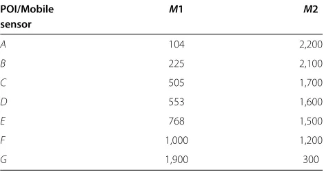
Table 1 The weight of edges

M1 M2 A B C D E F G H

M1 0 2,900 204 325 605 653 868 1,100 2,000 2,200

M2 2,900 0 2,050 2,000 1,600 1,500 1,400 1,100 313 100

A 204 2,050 0 120 463 595 821 1,000 1,900 2,100

B 325 2,000 120 0 400 586 831 976 1,800 2,000

C 605 1,600 463 400 0 300 507 585 1,400 1,600

D 653 1,500 595 586 300 0 300 440 1,400 1,500

E 868 1,400 821 831 507 300 0 290 1,300 1,400

F 1,100 1,100 1,000 976 585 440 290 0 1,000 1,100

G 2,000 313 1,900 1,800 1,400 1,400 1,300 1,000 0 200

(6)

Table 2 The 2MDkT after tentatively add every uncovered

Proof. According to SSR algorithm, firstly, there are|V| POIs needed to be added and only one POI can be added in each iteration. Secondly, after tentatively adding each POI to all the trajectories, the calculation of length dif-ference between the maximal and minimal trajectories in current mobile sensor network costsO(k|V|)time. There-fore, the computational complexity of the SSR algorithm isO(k|V|2₎_{. The proof finishes.}

5 Algorithms for the Minimum-Delay POIs Coverage problem without restriction

In this section, we will propose two algorithms for the Minimum-Delay POIs Coverage problem to deal with the scenario that the mobile sensors are not restricted to start sweeping from the determined positions, which is more flexible in practical applications.

5.1 TSP-based searching algorithm for the

Minimum-Delay POIs Coverage without restriction

In this subsection, we propose a TSP-based searching algorithm (TSP-Salgorithm). The main idea of the TSP-S algorithm is as follows: firstly, we create a weighted completed graph G = (V,E,W) shown as Section 3.2. Secondly, we use the TSP algorithm in [3] to find a TSP ring on G. Thirdly, we divide the TSP ring into k tra-jectories. Finally, each mobile sensor moves along one trajectory back and forth.

Similar as the notations defined in Section 4, we denote Cas a set of trajectories,C = {c1,c2,. . .,ck},ciis theith trajectory. Initially, setC= ∅.Trepresents the set of POIs which have not been covered byC. The input of the algo-rithm isG= (V,E,W). The output of the algorithm is a setC = {c1,c2,. . .,ck} of trajectories which contains all vertexes inV. Next, we present the TSP-S algorithm in details.

(1) SetC= ∅and set all POIs to be uncovered.

(2) InputG into the PTAS algorithm for TSP, and get an approximate TSP ring. The length of the TSP ring is|L|.

(3) Remove the current longest edgelmaxin the TSP

ring. We denote the left curve of the TSP ring aslcur,

|lcur|=|Lj|−|lmax|. Then we obtain a boundl,l= |lcur|/k,

k is the number of trajectories we aim to find. (4) Select one of the ends oflcur, and make it as the start

of establishing the current trajectoryj.

(5) Add POIs inlcurto the current trajectoryj in sequence

until the length ofj is larger than l, remove the last added POIi from j. Thus, we obtain the trajectory j and add it toC. And set the POIs in j to be covered. (6) Remove the edge between the POIi and the last POI

in trajectoryj, which is denoted asldel. Therefore,

of establishing the next trajectory and calculate the boundl again.

(7) Repeat steps (5) to (6) until the trajectories inC contains all POIs.

(8) When all POIs have been covered and the number of trajectories that have been found are less thank, then we will adjust the trajectories. We always choose the longest trajectoryw in C and split it into two trajectories evenly until we have obtainedk trajectories.

The pseudocode of the TSP-S algorithm is presented in Algorithm 2 and Algorithm 3.

Algorithm 2TSP-S(V,E,W,k,C) 1: SetC=φ;

2: ring←TSP(); 3: t=k,tcur=1; 4: lcur =ring.length; 5: lmax=max edge in ring; 6: lcur = |lcur| − |lmax|;

7: vcur=POI on the max edge in ring; 8: ctcur= {vcur},ltcur =0,C=C∪ctcur; 9: for(i=0 to ring.size()−1)do 10: vnext=ring.next();

11: if|ltcur| + |vcur,vnext|<= |lcur|/tthen 25: clongest←FindLongestTraj(); 26: cnew←SplitTraj(clongest);

27: C=C∪cnew;

(7)

Algorithm 3SplitTraj(clongest)

1: Letllongestdenote the longest trajectory inC. 2: h= |llongest|/2;

3: vcur =clongest.get(); 4: cnew=vcur; 5: lnew=0;

6: clongest=clongest− {vcur}; 7: whilelnew <hdo 8: vnext=clongest.next();

9: llongest= |llongest| − |vcur,vnext|; 10: clongest=clongest− {vnext}; 11: cnew=cnew∪vnext; 12: lnew=lnew+ |vcur,vnext|; 13: vcur =vnext;

14: end while

15: vnext=clongest.next();

16: llongest= |llongest| − |vcur,vnext|; 17: Returncnew;

In the following, we explain the TSP-S algorithm by two examples. In the first example, there are three mobile sen-sors and a set of POIs. Firstly, as shown in Figure 3a, we obtain a TSP ring and calculate the boundl. Secondly, as shown in Figure 3b, we remove the longest edge AJ in the ring and choose POIAas the start location to establish the first trajectory. We add POIB,C,D, andEto the trajec-tory in sequence. However, when adding POIEto the first trajectory, we find that the length of current trajectory is

larger than the boundl. Then, remove POIEfrom the tra-jectory and delete the edge DE from the ring as shown in Figure 3b. Thus, the first trajectory isL1 = {A,B,C,D}. Then, we calculate the boundlagain and start from POI E to repeat the above steps to establish the next trajec-tory. The next removed edge is GH as shown in Figure 3c. At last, three trajectories are generated, the second and third trajectories areL2= {E,F,G}andL3 = {H,I,J}as illustrated in Figure 3d. Let the three mobile sensors move along with the three trajectories, respectively.

Another example is shown in Figure 4 which is a spe-cial case for the TSP-S algorithm. There are four mobile sensors. However, when searching the third trajectory, all POIs in the region have been covered.

To solve this problem, we have to adjust the trajecto-ries as shown in Figure 4a. We choose the longest oneL1 among the three trajectories, and splitL1 into two parts L11 andL12. After the adjustment, as shown in Figure 4b, there are four trajectories for four mobile sensors at last.

Theorem 2. The time complexity of the TSP-S algorithm is O(|V|2), where|V|is the number of the POIs.

Proof.According to the TSP-S algorithm, firstly, creat-ing an approximateTSPring takesO(|V|2₎_{time. Secondly,} it costsO(|V|)to divide and adjust the TSP ring into k trajectories. Therefore, the time complexity of the TSP-S algorithm isO(|V|2). The proof finishes.

a

b

c

d

(8)

a

b

Figure 4A special case of POIs coverage for TSP-S.(a)Remove the edge BC from the longest trajectoryL1.(b)The longest trajectoryL1is splitted into two trajectoriesL11andL12, so there are four trajectories now.

5.2 Modified stretched searching algorithm for the Minimum-Delay POIs Coverage problem without restriction

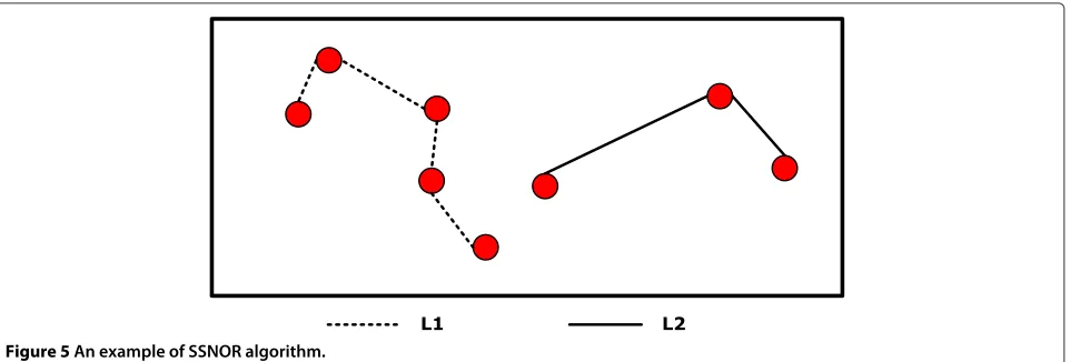
In this subsection, we modify the SSR algorithm to apply to the scenario that the start-positions of mobile sen-sors are not restricted. We propose an algorithm named SSNORfor this scenario.

In the following, we introduce the difference between the SSNOR and the SSR algorithms. In the SSR algorithm, the start locations of establishing trajectories are

deter-mined. In the SSNOR algorithm, there are only nPOIs

deployed in the region but no start positions of mobile sensors. We randomly selectkPOIs as the start locations of establishingktrajectories, we denote thesekrandomly selected POIs asPs = {ps1,. . .,psk}and set these POIs to covered.

After that, the rest operations are the same as that of in the SSR algorithm. We always choose the POI which minimizes the 2MDkT and add it to the trajectory. The procedure continues until all of the POIs have been added to the trajectories.

As shown in Figure 5, since the number of the mobile sensors is given, we generate two trajectories in the area. Apparently, the two mobile sensors can start sweeping

at arbitrary positions in their trajectories which is more flexible in practical applications.

6 Performance evaluation

In this section, we will evaluate the performance of the proposed algorithms by extensive simulations. We test two important metrics: the delay and the max-min dif-ference (2MDkT) of POIs Coverage schemes. The goal of the Minimum-Delay POIs Coverage problem is schedul-ing the given number of mobile sensors to monitor all POIs in the region and minimizing the delay. Since the length of each sensor’s trajectory is various, the time of sweeping is different from each other. Although a mobile sensor finishes sweeping, it cannot start the next round of sweeping immediately until all sensors finish sweeping. The max-min difference affects the monitoring efficiency. In Figures 6 and 7, we discuss the performance of our algorithms for two scenarios, respectively.

6.1 Simulation setup

In our simulations, the POIs and mobile sensors are ran-domly deployed in a 3,000 m×3,000 m square area. The moving velocityvof each mobile sensor is the same, which is 80 m/min. LetSdenote the number of mobile sensors,P

(9)

0

500 600 700 800 900 1000 1100 500 600 700 800 900 1000 1100

Th

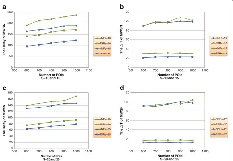
Figure 6The performance for the scenario with determined start positions.(a)The delay of the NNF and SSR algorithms whereS= 10 and 15. (b)TheTof the NNF and SSR algorithms whereS= 10 and 15.(c)The delay of the NNF and SSR algorithms whereS= 20 and 25.(d)TheTof the NNF and SSR algorithms whereS= 20 and 25.

denote the number of POIs. The positions of all POIs are known in advance.

Since the moving velocity v of mobile sensors is the same, the 2MDkT of the minimum POIs coverage is equivalence to theT, which is defined as the time inter-val from the first sensor accomplishing the sweeping to the last sensor finishing sweeping (T = 2MDkT/v). As far as we know, none of the previous works about POIs coverage considered the restriction on the num-ber of mobile sensors and the start position restriction; therefore, we compare the SSR algorithm with a greedy algorithm called Nearest Neighbor First (NNF) algorithm. In the NNF algorithm, a nearest neighboring POI of each mobile sensor is always selected to add to the correspond-ing trajectory. In the second scenario, without the deter-mined start positions, a Nearest Neighbor Prior algorithm

(UNNP) is compared with TSP-S and SSNOR algorithms.

Furthermore, we compare our TSP-S algorithm with the existing OSWEEP [2] algorithm.

For each simulation setting, we run 100 times and take the average value as the final results.

6.2 The performance of the SSR algorithm

To evaluate the performance of the SSR algorithm, we change the number of POIs and measure the delay andT with the given number of mobile sensors. We setS= 10, 15, 20, and 25 in Figure 6a,b,c,d, respectively. Firstly, we can observe that increasing the number of mobile sensors can improve the performance of the SSR algorithm signif-icantly. This is because the number of POIs assigned to each mobile sensor is decreased with more mobile sen-sors sweeping. However, the performance of NNF largely depends on the deployment of POIs, increasing the num-ber of mobile sensors can not ensure the performance is improved.

(10)

0

500 600 700 800 900 1000 1100 500 600 700 800 900 1000 1100

500 600 700 800 900 1000 1100

UNNP

Figure 7The performance for the scenario with undetermined start positions.(a)The delay of the UNNP, SSNOR, and TSP-S algorithms where S= 10.(b)TheTof the UNNP, SSNOR, and TSP-S algorithms whereS= 10.(c)The delay of the UNNP, SSNOR, and TSP-S algorithms whereS= 15. (d)TheTof the UNNP, SSNOR, and TSP-S algorithms whereS= 15.(e)The delay of the UNNP, SSNOR, and TSP-S algorithms whereS= 20.(f)The

(11)

a

b

c

d

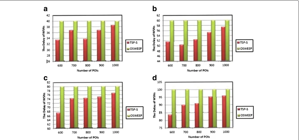
Figure 8The comparison between the TSP-S algorithm and the OSWEEP algorithm.(a)The delay limitation of OSWEEP is set as 40 min.(b)The delay limitation of OSWEEP is set as 60 min.(c)The delay limitation of OSWEEP is set as 80 min.(d)The delay limitation of OSWEEP is set as 100 min.

equal, but it can not ensure that the length of sweeping trajectories is approximately equal.

Thirdly, since the size of region is fixed, when the num-ber of POIs increasing, the length of each trajectory does not change too much. As shown in Figure 6, the fluctu-ation of the delay and T is slight. Therefore, we can

conclude that the delay and T of the SSR algorithm

change little when the number of POIs increasing.

6.3 The performance of the TSP-S algorithm and the SSNOR algorithm

We compare the delay andTof TSP-S and SSNOR with

UNNP. We employ 10, 15, 20, and 25 mobile sensors. As shown in Figure 7, it is obvious that the TSP-S and SSNOR outperform the UNNP. Furthermore, the TSP-S algorithm has better performance than the SSNOR algorithm. It is because SSNOR algorithm only considers local efficiency, while the TSP-S algorithm considers global efficiency.

We can also observe that with the increasing ofS, the

delay andT of TSP-S and SSNOR decrease. When the

number of POIs increases, the delay andTof the TSP-S and SSNOR have slight change because the length of each trajectory changes a little.

6.4 The comparison between the TSP-S algorithm and the OSWEEP algorithm

We compare our TSP-S algorithm with the existing algo-rithm OSWEEP [2]. Since the OSWEEP addressed the Minimum Mobile sensor problem under the sweep delay limitation, which is different from ours, we first set the sweep delay as 40, 60, 80, and 100 min under the different

number of POIs for OSWEEP, respectively, and obtain the corresponding minimum number of mobile nodes, named S, by the OSWEEP algorithm. Then we set the number of mobile nodes for our algorithm asSto com pare the sweep delay of the two algorithms. As shown in Figure 8, we can observe that the sweep delay of our TSP-S algorithm is always lower than the OSWEEP’s. The delay difference of the two algorithms is 17% at most and 9% averagely. It is because the TSP-S algorithm remove the longer edge from the TSP ring when generating the trajectory of each mobile sensor which reduces the sweep distance and time.

7 Conclusion

(12)

Competing interests

The authors declare that they have no competing interests.

Authors’ contributions

WPC and SC surveyed the literature and prepared the draft. DYL provided guidelines for the review. All authors read and approved the final manuscript.

Acknowledgements

This research was jointly supported in part by the National Natural Science Foundation of China under grants 61070191 and 91124001 and the Research Fund for the Doctoral Program of Higher Education of China under grant 20100004110001.

Received: 28 December 2012 Accepted: 22 October 2013 Published: 11 November 2013

References

1. M Li, W-F Cheng, K Liu, Y Liu, X-Y Li, X Liao, Sweep coverage with mobile sensors. IEEE Trans. Mob. Comput.10(11), 1534–1545 (2011)

2. J Du, Y Li, H Liu, K Sha, inICPADS. On sweep coverage with minimum mobile sensors (Shanghai, 8-10 Dec 2010)

3. G Nicosia, Worst-case analysis of a new heuristic for the travelling salesman problem. Technical Report 388, Graduate School of Industrial Administration, Carnegie Mellon University, (1976)

4. M Cardei, D-Z Du, Improving wireless sensor network lifetime through power aware organization. Wireless Netw.11(3), 333–340 (2005) 5. M Cardei, MT Thai, Y Li, W Wu, inINFOCOM. Energy-efficient target

coverage in wireless sensor networks (Miami, 13–17 March 2005) 6. H Liu, W Chen, H Ma, D Li, inWASA. Energy-efficient algorithm for the

target q-coverage problem in wireless sensor networks (Beijing, 15–17 Aug 2010)

7. H Liu, P-J Wan, C-W Yi, X Jia, SAM Makki, N Pissinou, inINFOCOM. Maximal lifetime scheduling in sensor surveillance networks (Miami, 13–17 March 2005)

8. M Chaudhary, AK Pujari, inICDCN. Q-coverage problem in wireless sensor networks (Hyderabad, 3–6 January 2009)

9. M Cardei, D MacCallum, MX Cheng, M Min, X Jia, D Li, D-Z Du, Wireless sensor networks with energy efficient organization. J. Interconnection Netw.3(3–4), 213–229 (2002)

10. S Slijepcevic, M Potkonjak, inICC. Power efficient organization of wireless sensor networks (Helsinki, 11-14 June 2001)

11. X Bai, D Xuan, Z Yun, T-H Lai, W Jia, inMobiHoc. Complete optimal deployment patterns for full-coverage and k-connectivity (k<=6) wireless sensor networks (Hong Kong, 27–30 May 2008) 12. S Kumar, T-H Lai, J Balogh, inMOBICOM. On k-coverage in a mostly

sleeping sensor network (Philadelphia, 26 September - 1 October 2004) 13. X Wang, G Xing, Y Zhang, C Lu, R Pless, CD Gill, inSenSys. Integrated

coverage and connectivity configuration in wireless sensor networks (Los Angeles, 5–7 November 2003)

14. B Liu, P Brass, O Dousse, P Nain, DF Towsley, inMobiHoc. Mobility improves coverage of sensor networks (Urbana-Champaign, 25–28 May 2005) 15. Z Zhou, SR Das, H Gupta, inICCCN. Connected k-coverage problem in

sensor networks (Chicago, 11–13 October 2004)

16. M Hefeeda, M Bagheri, inINFOCOM. Randomized k-coverage algorithms for dense sensor networks (Anchorage, 6–12 May 2007)

17. Y Wang, G Cao, inINFOCOM. On full-view coverage in camera sensor networks (Shanghai, 10–15 April 2011)

18. X Bai, S Kumar, D Xuan, Z Yun, T-H Lai, inMobiHoc. Deploying wireless sensors to achieve both coverage and connectivity (Florence, 22–25 May 2006)

19. S Kumar, T-H Lai, A Arora, inMOBICOM. Barrier coverage with wireless sensors (Cologne, 26 August - 2 September 2005)

20. A Chen, S Kumar, T-H Lai, inMOBICOM. Designing localized algorithms for barrier coverage (Montreal, 9–14 September 2007)

21. P Balister, B Bollobás, A Sarkar, S Kumar, inMOBICOM. Reliable density estimates for coverage and connectivity in thin strips of finite length (Montreal, 9–14 September 2007)

22. H Yang, D Li, Q Zhu, W Chen, Y Hong, inWASA. Minimum energy cost k-barrier coverage in wireless sensor networks (Beijing, 15–17 August 2010)

23. K-F Ssu, W-T Wang, F-K Wu, T-T Wu, K-barrier coverage with a directional sensing model. Smart Sensing Intell. Syst.2(1), 75–93 (2009)

24. A Saipulla, C Westphal, B Liu, J Wang, inINFOCOM. Barrier coverage of line-based deployed wireless sensor networks (Rio de Janeiro, 19–25 April 2009)

25. B Liu, O Dousse, J Wang, A Saipulla, inMobiHoc. Strong barrier coverage of wireless sensor networks (Hong Kong, 26–30 May 2008)

26. S He, J Chen, X Li, X Shen, Y Sun, inINFOCOM. Cost-effective barrier coverage by mobile sensor networks (Orlando, 25–30 March 2012) 27. W Wang, V Srinivasan, KC Chua, inMOBICOM. Trade-offs between mobility

and density for coverage in wireless sensor networks (Montreal, 9–14 September 2007)

28. D Wang, J Liu, Q Zhang, inIEEE IWQoS. Probabilistic field coverage using a hybrid network of static and mobile sensors (Evanston, 21–22 June 2007) 29. E Ekici, Y Gu, D Bozdag, Mobility-based communication in wireless sensor

networks. IEEE Commun. Mag.44(7), 56–62 (2006)

30. S Chellappan, W Gu, X Bai, D Xuan, B Ma, K Zhang, Deploying wireless sensor networks under limited mobility constraints. IEEE Trans. Mob. Comput.6(10), 1142–1157 (2007)

31. S Arora, inFOCS. Polynomial time approximation schemes for Euclidean TSP and other geometric problems (Burlington, 14–16 October 1996)

doi:10.1186/1687-1499-2013-262

Cite this article as:Chenet al.:Minimum-Delay POIs Coverage in mobile

wireless sensor networks.EURASIP Journal on Wireless Communications and

Networking20132013:262.