Threshold dynamics of a delayed predator–prey model with impulse via the basic reproduction number

(1)

R E S E A R C H

Open Access

Threshold dynamics of a delayed

predator–prey model with impulse via the

basic reproduction number

Xiangsen Liu

1*

_{and Binxiang Dai}

2

*_{Correspondence:}

[email protected]

1_{Department of Mathematics,}

North University of China, Taiyuan, P.R. China

Full list of author information is available at the end of the article

Abstract

In this paper, we study a delayed predator–prey model with impulse and, in particular, the existence of the predator-free periodic solution. We employ the approach and techniques coming from epidemiology and calculate the basic reproduction number for the predator. Using the basic reproduction number, we consider the global attraction of the predator-free periodic solution and uniform persistence of the predator. Our results improve the results by Li and Liu (Adv. Diﬀer. Equ. 2016:42,2016), where they left the open problem of ﬁnding a threshold value that determines the eradication and uniform persistence of the predator. Furthermore, we give some numerical simulations to illustrate our results.

Keywords: Predator–prey model; Delay; Impulse; Basic reproduction number

1 Introduction

In the natural world, many species usually pass through a number of stages during their life cycle. So it is practical to introduce time delay into models of theoretical ecology. In par-ticular, it is often important to take into account the processes of gestation and maturation to make an abstract model more biologically realistic [2–4]. The characteristic property of population models with time delay is their oscillatory behavior: for a sufficiently large mat-uration period, an initially stable equilibrium becomes unstable, and the system exhibits sustained oscillations [2,5]. Additionally, impulsive differential equations have been ex-tensively used as models in biology, physics, chemistry, engineering, and other sciences with particular emphasis on population dynamics [6–9]. In [9] the authors discussed an impulsive predator–prey system with stage structure and generalized functional response. Sufficient conditions are established for the existence of a predator-free positive periodic solution and the permanence of the system. Numerical simulation shows that impulses and functional response affect the dynamics of the system.

(2)

authors considered the following delayed model with impulse:

wherex(t) andy(t) denote the population densities of prey and predator at timet, respec-tively,r,K,α,β,k,dare positive,ris the intrinsic rate of increase of the prey,Kis the carrying capacity of the prey,αis the predation coeﬃcient of the predator, which reﬂects the size of the predator’s ability, β is the predation regulation factor (saturation factor) of the predator, dis the death rate of the predator,k(0 <k< 1) is the rate of convers-ing prey into predator,τ > 0 denotes a time delay due to the gestation of the predator,

x(t) =x(t+_{) –}_x₍_t_),_y₍_t_{) =}_y₍_t+_{) –}_y₍_t_),_T _{is the impulsive period,}_n_∈_N

+={1, 2, . . .}, and

p> 0 is the proportionality constant, which represents the rate of mortality due to the applied pesticide. The initial conditions for system (1.1) are

φ1(s),φ2(s)

∈C [–τ, 0],R2₊, φi(0) > 0 (i= 1, 2). (1.2)

In [1], suﬃcient conditions for the global attraction of a predator-free periodic solu-tion are obtained by the theory of impulsive diﬀerential equasolu-tions, that is,T <T₁∗. The conditions for the permanence of the system are investigated, that is,T>T₂∗. Note that

T₁∗<T₂∗always holds. It is obvious that ifT∈(T₁∗,T₂∗), then we cannot determine whether the predator can persist or not. In the present paper, we give a thorough global dynam-ics of (1.1), which completely solves the question left in [1]. To do this, we employ the approach coming from epidemiology [13]. As far as we know, there are no papers em-ploying this approach in ecology. Throughout the present paper, roughly speaking, the basic reproduction numberR0 may be thought as the number of predators one preda-tor gives rise during its life, when introduced in a prey population [14]. A similar thresh-old value for the coexistence of a predator–prey system has previously been formulated and explained by Pielou [15], among others but, to the best of our knowledge, has not been termed a “basic reproduction number.” In ecology, many authors have investigated the autonomous predator–prey systems using the basic reproduction number [16,17]. For example, in [16] the authors considered a stage-structured predator–prey model with nonlinear predation rate. They discussed the stability of the system using the basic re-production number of the predator population. In contrast, there have been few papers discussing the nonautonomous, delayed, or impulsive predator–prey systems using the basic reproduction number (except for [18]). In [18] the authors considered an ecoepi-demiological model with Holling type-III functional response and time delay. They used the ecological and disease basic reproduction numbers to determine the persistence of the system. In this paper, using the basic reproduction number of the predator population and approach in [13], we wish to ﬁnd a threshold value to determine whether the predator can exist or not.

(3)

we employ the approach coming from epidemiology and calculate the basic reproduction number for the predator. In Sect.4, using the basic reproduction number, we consider the global attraction of the predator-free periodic solution and persistence of the predator in (1.1). In Sect.5, we give some numerical simulations to illustrate our results. Finally, we give some concluding remarks.

2 The existence of a predator-free periodic solution and boundedness of system (1.1)

In this section, we investigate the existence of a predator-free periodic solution of system (1.1). In this case, the predator population is entirely absent from the population perma-nently, that is,y(t) = 0,t≥0. System (1.1) yields

⎧ ⎨ ⎩

x(t) =rx(t)(1 –x_K(t)), t=nT,

x(t) = –px(t), t=nT.

(2.1)

For system (2.1), we have the following result.

Lemma 2.1([1]) If(1 –p)erT_{> 1,}_{then system}₍_2.1₎_{has the unique positive periodic solution}

x∗(t) = x

∗

0

(1 –x∗₀/K)e–r(t–nT)₊_x∗ 0/K

, t∈ nT, (n+ 1)T, (2.2)

which is globally asymptotically stable,where

x∗₀=K((1 –p)e

rT_{– 1)}

erT_{– 1} . (2.3)

According to Lemma2.1, we obtain the following result.

Theorem 2.1 If (1 –p)erT _{> 1,}_{then system} ₍_1.1₎_{has a predator-free periodic solution}

(x∗(t), 0),where x∗(t)is shown in(2.2).

Next, we will show that all solutions of (1.1) are uniformly upper bounded.

Theorem 2.2 If(1 –p)erT_{> 1,}_{then all solutions of}₍_1.1₎_{are uniformly upper bounded}_. Proof From the ﬁrst and third equations of (1.1) we have

⎧ ⎨ ⎩

x(t)≤rx(t)(1 –x_K(t)), t=nT,

Consider the following impulsive comparison system:

⎧ ⎨ ⎩

z₁(t) =rz1(t)(1 –z1_K(t)), t=nT,

z1(t) = –pz1(t), t=nT.

(2.4)

(4)

for given0> 0, there existsT1> 0 such that, fort>T1,

x(t)≤z1(t)≤x∗(t) +0≤

x∗₀

(1 –x∗₀/K)e–rT₊_x∗

0/K

+0M1. (2.5)

LetV(t) =kx(t–τ) +y(t). Then, fort>T1+τ, we have

V(t) =krx(t–τ)

1 –x(t–τ)

K

–dy(t)

≤krx(t–τ) –dy(t)

= (kr+kd)x(t–τ) –d kx(t–τ) +y(t)

≤k(r+d)M1–dV(t)

and

V (nT+τ)+=kxnT++y (nT+τ)+

=k(1 –p)x(nT) +y(nT+τ)

≤kx(nT) +y(nT+τ)

=V(nT+τ).

⎧ ⎨ ⎩

V₁(t) =k(r+d)M1–dV1(t), t=nT+τ,

V1(t) = 0, t=nT+τ.

It is clear that

lim

t→+∞V1(t) =

k(r+d)M1

d .

By the comparison principle, for0> 0, there existsT2>T1+τ such that, fort>T2, we get

V(t)≤V1(t)≤

k(r+d)M1

d +0M2. (2.6)

The proof is completed.

Thus the dynamics of system (1.1) can be analyzed in the following bounded feasible region:

Γ = x(t),y(t)|0≤x(t)≤M1, 0≤y(t)≤M2

,

(5)

3 The basic reproduction number of the predator

In this section, we introduce the basic reproduction numberR0of the predator for system (1.1) using the next generation operators approach in [19]. We linearize system (1.1) at (x∗(t), 0) and get

y(t) = kαx

∗2₍_t_–_τ₎

1 +βx∗2₍_t_–_τ₎y(t–τ) –dy(t)

=g(t)y(t–τ) –dy(t), (3.1)

where

g(t) = kαx

∗2₍_t_–_τ₎

1 +βx∗2₍_t_–_τ₎. (3.2)

From (3.1) we obtain

y(t) =y(0)e–dt+e–dt t

0

g(s)y(s–τ)edsds.

Lety1(t) =g(t)y(t–τ). Then

y1(t) =y(0)g(t)e–d(t–τ)+e–d(t–τ)g(t)

t–τ

0

y1(s)edsds.

Making the change of variables=t–δ, we get

y1(t) =y(0)g(t)e–d(t–τ)+g(t)e–d(t–τ)

t

τ

y1(t–δ)ed(t–δ)dδ

=y(0)g(t)e–d(t–τ)+g(t)

t

τ

y1(t–δ)e–d(δ–τ)dδ

=y10(t) +

t

τ

¯

K(t,δ)y1(t–δ) dδ,

where

y10(t) =y(0)g(t)e–d(t–τ)

and

¯

K(t,δ) =

⎧ ⎨ ⎩

0, δ<τ,

g(t)e–d(δ–τ)_, _δ_≥_τ_.

LetCTbe the ordered Banach space of all continuousT-periodic functions fromRto Requipped with the maximum norm · and the positive coneC+

T={ψ ∈CT|ψ(t)≥

0,t∈R}. Then we can deﬁne the linear operatorL:CT→CTby

L:v(t)→

+∞

0

¯

(6)

Following [19], the basic reproduction number of the predator is deﬁned asR0r(L), the spectral radius ofL.

We see that the basic reproduction numberR0=r(L) can be obtained by solving the eigenvalue problem

Diﬀerentiating Eq. (3.3) and then integrating by parts, we have

R0u(t) =g(t)

This equation can be rewritten as

u(t)

Obviously, there is no explicit formula forR0whenτ= 0.

Remark3.1 Whenτ= 0, system (1.1) reduces to a periodic system of ordinary diﬀerential equations. The corresponding basic reproduction numberR0becomes

R0=

T

0 g(t) dt

dT .

4 The global dynamics of system (1.1)

In this section, we study the global dynamics of system (1.1) in terms of its basic repro-duction numberR0. To this end, we ﬁrst introduce some lemmas for our main results.

For anyψ∈C([–τ, 0],R), letP(t)ψ=ut(ψ) be the unique solution of (3.1) satisfying

Consider the following linear equation with time delay:

(7)

wherea(t)∈CT, andb(t) is a piecewise left-continuousT-periodic function with discon-tinuous points of ﬁrst kind atnTsuch thatb(t) > 0,t≥0. By applying the method of steps it is easy to verify that, for anyφ∈C+=C([–τ, 0],R+), system (4.1) has a unique contin-uous solutionu(t,φ) on [–τ, +∞) withu0=φ. LetPbe the Poincaré map associated with (4.1) onC+, that is,P(φ) =uT(φ). Then we have the following result.

Lemma 4.2 [13].Letμ=lnr(_TP).Then there exists a positive T -periodic function v(t)such that eμt_v₍_t₎_{is a solution of} ₍_4.1_).

For the predator-free periodic solution (x∗(t), 0) of (1.1), we have the following result.

Theorem 4.1 Assume that(1 –p)erT_{> 1.}_{If R}

0< 1,then the predator-free periodic solution (x∗(t), 0)of (1.1)is globally attracting,where R0is deﬁned in(3.5).

Proof LetPbe the Poincaré map of the following perturbed linear equation:

y₂(t) = kα(x

∗₍_t_–_τ_{) +}₎2

1 +β(x∗(t–τ) +)2y2(t–τ) –dy2(t). (4.2)

By Lemma4.1we see thatR0< 1 if and only ifr(P) < 1, wherePis the Poincaré map of (3.1). Sincelim→0r(P) =r(P) < 1, we may ﬁx a small enough> 0 such thatr(P) < 1.

By Lemma4.2there is a positiveT-periodic functionv(t) such thateμtv(t) is a positive

solution of (4.2), whereμ=lnr_T(P)< 0.

According to the proof of Theorem2.2, for given> 0, there existsT3> 0 such that, for

t>T3,

x(t)≤x∗(t) +, (4.3)

wherex∗(t) is deﬁned in (2.2).

By the second equation of (1.1), fort>T3+τ, we get

y(t)≤ kα(x

∗₍_t_–_τ_{) +}₎2

1 +β(x∗(t–τ) +)2y(t–τ) –dy(t).

Choose a suﬃciently large A> 0 such that y(t)≤Aeμt_v

(t), t∈[T3,T3 +τ], where

Aeμt_v

(t) is a positive solution of (4.2). By the comparison principle we have y(t)≤Aeμt_v

(t), t≥T3+τ.

Sinceμ< 0,limt→+∞y(t) = 0.

Then for a suﬃciently small1> 0 (1<αMr1, whereM1is shown in (2.5)), there exists

T4> 0 such that, fort>T4, we obtain

0 <y(t) <1.

From the ﬁrst and third equations of (1.1), fort>max{T1,T4}, we have

⎧ ⎨ ⎩

x(t)≥x(t)(r–αM11–_Krx(t)), t=nT,

(8)

⎧ ⎨ ⎩

z₂(t) =z2(t)(r–αM11–_Krz2(t)), t=nT,

z2(t) = –pz2(t), t=nT.

(4.4)

Since1< αMr1, it is obvious thatr–αM11> 0. According to Lemma2.1, we ﬁnd that

system (4.4) has a globally asymptotically stable periodic solution

z₂∗(t) = z

∗

2(0+)

(1 –rz∗₂(0+)/(Kr1))e–r1(t–nT)+rz∗2(0+)/(Kr1)

, nT<t≤(n+ 1)T,

with

z₂∗(0+) =Kr1((1 –p)e

r1T_{– 1)}

r(er1T_{– 1)} , r1=r–αM11.

By the comparison principle, forx(0+)≥z2(0+) andt>max{T1,T4}, we havex(t)≥z2(t), andz2(t) –z∗2(t)→0 ast→+∞. Meanwhile,z∗2(t) –x∗(t)→0 as1→0. Based on this analysis and (4.3), we see thatx(t) –x∗(t)→0 ast→+∞. Therefore the predator-free periodic solution (x∗(t), 0) of (1.1) is globally attracting. The proof is completed.

Theorem 4.2 Let(1 –p)erT _{> 1.}_{If R}

0> 1,then there exists q> 0such that every positive

solution(x(t),y(t))of (1.1)satisﬁes y(t)≥q for t large enough.

Proof LetMηbe the Poincaré map of the perturbed equation

¯

y(t) = kα(x

∗₍_t_–_τ_{) –}_η₎2

1 +β(x∗(t–τ) –η)2y¯(t–τ) –dy¯(t). (4.5)

Sincelimη→0r(Mη) =r(P) > 1, we can ﬁx a small positive numberηsuch thatr(Mη) > 1

andη<inf_t≥0x∗(t).

By Lemma4.2there is a positiveT-periodic functionvη(t) such thateμηtvη(t) is a positive

solution of (4.5), whereμη=

lnr(Mη)

T > 0.

Consider the impulsive comparison system

⎧ ⎨ ⎩

¯

x(t) =x¯(t)(r–αM1¯–_Krx¯(t)), t=nT,

x¯(t) = –px¯(t), t=nT. (4.6)

where 0 <¯<_α_Mr

1, andM1is shown in (2.5).

Using Lemma2.1, we see that system (4.6) admits a positive periodic solutionx∗_¯(t), which is globally asymptotically stable, andlim¯→0x∗¯(t) =x∗(t). Hence we can ﬁx a small

number¯∈(0,_α_Mr

1) such that, fort≥0,

x∗_¯(t) >x∗(t) – η

2. (4.7)

(9)

y(t) <γ fort>t0. It follows from the ﬁrst equation of (1.1) that, fort>t0,

x(t)≥rx(t)

1 –x(t)

K

–αM1γx(t)

≥x(t)

r–αM1¯–

rx(t)

K

.

Therefore we have

⎧ ⎨ ⎩

x(t)≥x(t)(r–αM1¯–rx_K(t)), t=nT,

By system (4.6) and the comparison principle there existst1>t0such that, fort>t1and

x(0+)≥ ¯x(0+),

x(t)≥ ¯x(t) >x∗_¯(t) – η

2. (4.8)

Using (4.7) and (4.8), fort>t1, we get

x(t) >x∗(t) –η. (4.9)

From (4.9) and the second equation of (1.1), fort>t2t1+τ, we have

y(t)≥ kα(x

∗₍_t_–_τ_{) –}_η₎2

1 +β(x∗(t–τ) –η)2y(t–τ) –dy(t). (4.10)

Choose a numberm1> 0 such that

y(t)≥m1eμηtvη(t), t∈[t1,t2], (4.11)

and

m1eμηtvη(t) <γ, t∈[t1,t2], (4.12)

whereeμηt_v

η(t) is a positive solution of (4.5) andμη> 0. Using (4.10), (4.11), (4.12), and the

comparison theorem, there must bet3>t2such thatγ<y(t3) <¯, which is a contradiction. From the above claim we discuss the following two possibilities:

(H1) y(t)≥γ for all larget.

(H2) y(t)oscillates aboutγ for all larget.

Letq=min{γ

2,q2}, where

q2=

q1mint∈[0,T]vη(t) eμητ_max

t∈[0,T]vη(t)

withq1=γe–dτ.

We hope to show thaty(t)≥qfortlarge enough. Obviously, we only need to consider case (H2). Lettand¯tsatisfy

(10)

wheretis suﬃciently large such that, fort∈[t,¯t],

x(t) >x∗(t) –η. (4.14)

Note that the function y(t) for t≥0 is uniformly continuous since its derivative is bounded for allt≥0. Hence there existsT(0 <T<τ is independent of the choice of

t) such thaty(t) >γ₂ fort∈[t,t+T]. Let us consider the following three cases: Case (B1)t¯–t≤T. Theny(t) >γ₂ for allt∈[t,t¯].

Case (B2)T<¯t–t≤τ.

By the second equation of (1.1) we have

y(t)≥–dy(t).

Using the comparison principle, fort∈[t,¯t], we get

y(t)≥y(t)e–d(t–t)

≥γe–dτ_q

1.

Therefore, in this case,y(t)≥q1fort∈[t,¯t]. Case (B3)t¯–t>τ.

Similarly to the discussion of case (B2), we obtainy(t)≥q1fort∈[t,t+τ]. Ify(t)≥q1 fort∈[t+τ,¯t], then our aim is reached. Suppose not. Then there existsT¯1> 0 such that

y(t)≥q1, t∈[t,t+τ+T¯1],

y(t+τ+T¯1) =q1, y(t) <q1, 0 <t– (t+τ+T¯1)1.

By (4.14) and the second equation of system (1.1), fort∈[t,¯t], we have

y(t)≥ kα(x

∗₍_t_–_τ_{) –}_η₎2

1 +β(x∗(t–τ) –η)2y(t–τ) –dy(t).

Choose a numberm2=q1[eμη(t+τ+T¯1)maxt∈[0,T]vη(t)]–1> 0. It is clear that, fort∈[t+

¯

T1,t+τ+T¯1],

m2eμηtvη(t)≤q1≤y(t),

and fort∈[t+T¯1,t¯],

m2eμηtvη(t)≥m2eμη(t+T¯1) min

t∈[0,T]vη(t) =

q1mint∈[0,T]vη(t) eμητ_max_t∈

[0,T]vη(t)

=q2> 0.

The comparison theorem implies that, fort∈[t+T¯1,¯t],

y(t)≥q2.

Thusy(t)≥q2fort∈[t,¯t].

(11)

5 Numerical simulation

In this section, we give phase portraits of system (1.1) to illustrate the above theoretical analysis using numerical simulations. We consider the following delayed model with im-pulse: cluded that ifT<T₁∗, then the predator-free periodic solution is globally attractive, and if

T>T₂∗, then the predator will persist. However, ifT∈(T₁∗,T₂∗), then they could not deter-mine whether the predator can persist or not. In the present paper, we completely solve this question.

By Eq. (3.3), for system (5.1), the following eigenvalue problem can be obtained:

g1(t)

+∞

0.5

u(t–δ)e–0.24(δ–0.5)dδ=R0u(t), u∈CT, (5.2)

whereR0andu(t) are the eigenvalue and eigenvector of Eq. (5.2), respectively, and

(12)

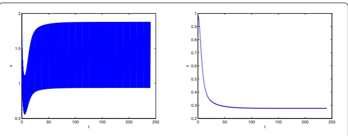
Figure 2Time series of the solution of system (5.1) withT= 0.7

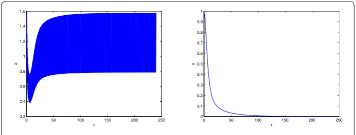
In system (5.1), letT= 0.6∈(T₁∗,T₂∗). We compute the basic reproduction numberR0 numerically to get R0≈0.8590 < 1. We also numerically compute the thresholdT∗≈ 0.6445. It is obvious thatT= 0.6 <T∗, that is,R0< 1. By Theorem4.1we obtain that the predator-free periodic solution is globally attractive. Figure1illustrates our theoretical results.

LetT= 0.7∈(T1∗,T2∗). We numerically compute the basic reproduction numberR0≈ 1.1250 > 1. It is clear thatT= 0.7 >T∗, that is,R0> 1. By Theorem4.2we obtain that the predator will become permanent. Figure2illustrates our theoretical results.

6 Conclusion

In this paper, we mainly discuss the extinction and permanence of the predator for system (1.1). Using the basic reproduction number coming from epidemiology, we may ﬁnd the threshold valueR0such that ifR0< 1, then the predator is extinct, whereas ifR0> 1, then it will persist. Thus we improve the results of [1]. As far as we know, this is the ﬁrst paper employing this approach of [13] in ecology.

Acknowledgements

We would like to thank the anonymous referees very much for their valuable comments and suggestions.

Funding

The research was supported by the National Natural Foundation of China (11271371, 51479215, 11571324).

Competing interests

The authors declare that they have no competing interests.

Authors’ contributions

Both authors contributed equally to the writing of this paper. Both authors read and approved the ﬁnal manuscript.

Author details

1_{Department of Mathematics, North University of China, Taiyuan, P.R. China.}2_{School of Mathematics and Statistics,}

Central South University, Changsha, P.R. China.

Publisher’s Note

Springer Nature remains neutral with regard to jurisdictional claims in published maps and institutional aﬃliations.

Received: 14 May 2018 Accepted: 19 November 2018

References

1. Li, S.Y., Liu, W.W.: A delayed Holling type III functional response predator–prey system with impulsive perturbation on the prey. Adv. Diﬀer. Equ.2016, 42 (2016).https://doi.org/10.1186/s13662-016-0768-8

(13)

4. Murdoch, W.W., Briggs, C.J., Nisbet, R.M.: Consumer-Resource Dynamics. Princeton University Press, Princeton (2003) 5. Ruan, S.G.: On nonlinear dynamics of predator–prey models with discrete delay. Math. Model. Nat. Phenom.4,

140–188 (2009)

6. Hui, J., Zhu, D.: Dynamic complexities for prey-dependent consumption integrated pest management models with impulsive eﬀects. Chaos Solitons Fractals29, 233–251 (2006)

7. Liu, B., Zhang, Y., Chen, L.S.: The dynamical behaviors of a Lotka–Volterra predator–prey model concerning integrated pest management. Nonlinear Anal., Real World Appl.6, 227–243 (2005)

8. Zhang, H., Georgescu, P., Chen, L.S.: An impulsive predator–prey system with Beddington–Deangelis functional response and time delay. Int. J. Biomath.1, 1–17 (2008)

9. Shao, Y.F., Li, Y.: Dynamical analysis of a stage structured predator–prey system with impulsive diﬀusion and generic functional response. Appl. Math. Comput.220, 472–481 (2013)

10. Liu, X., Ballinger, G.: Boundedness for impulsive delay diﬀerential equations and applications to population growth models. Nonlinear Anal., Theory Methods Appl.53, 1041–1062 (2003)

11. Leonid, B., Elena, B.: Linearized oscillation theory for a nonlinear delay impulsive equation. J. Comput. Appl. Math.161, 477–495 (2003)

12. Yan, J.: Stability for impulsive delay diﬀerential equations. Nonlinear Anal., Theory Methods Appl.63, 66–80 (2005) 13. Bai, Z.G.: Threshold dynamics of a time-delayed SEIRS model with pulse vaccination. Math. Biosci.269, 178–185

(2015)

14. Garrione, M., Rebelo, C.: Persistence in seasonally varying predator–prey systems via the basic reproduction number. Nonlinear Anal., Real World Appl.30, 73–98 (2016)

15. Pielou, E.C.: Introduction to Mathematical Ecology. Wiley-Interscience, New York (1969)

16. Paul, G., Hsieh, Y.H., Zhang, H.: A Lyapunov functional for a stage-structured predator–prey model with nonlinear predation rate. Nonlinear Anal., Real World Appl.11, 3653–3665 (2010)

17. Bate, A.M., Hilker, F.M.: Predator–prey oscillations can shift when diseases become endemic. J. Theor. Biol.316, 1–8 (2013)

18. Xu, R., Tian, X.H.: Global dynamics of a delayed eco-epidemiological model with Holling type-III functional response. Math. Methods Appl. Sci.37, 2120–2134 (2014)

19. Bacaër, N., Guernaoui, S.: The epidemic threshold of vector-borne diseases with seasonality. J. Math. Biol.53, 421–436 (2006)