T
HE
L
ONDON
S
CHOOL OF
E
CONOMICS AND
P
OLITICAL
S
CIENCE
Essays in Applied Macroeconomics
Łukasz Rachel
A thesis submitted to the Department of Economics of
the London School of Economics for the degree of
Doctor of Philosophy.
Declaration
I certify that the thesis I have presented for examination for the PhD degree of the London School of Economics and Political Science is solely my own work other than where I have clearly indicated that it is the work of others (in which case the extent of any work carried out jointly by me and any other person is clearly identified in it).
The copyright of this thesis rests with the author. Quotation from it is permitted, provided that full acknowledgement is made. This thesis may not be reproduced without my prior written consent.
I warrant that this authorisation does not, to the best of my belief, infringe the rights of any third party.
I declare that my thesis consists of approximately 55,000 words.
Statement of conjoint work
Acknowledgements
I wish to express my gratitude to people that accompanied me through this journey. I cannot find enough words to thank my advisor, Ricardo Reis, whose passion, enthusiasm, knowledge and mentorship have been incredibly inspiring. I am also grateful to the rest of the faculty at the LSE, and in particular to Francesco Caselli, Wouter den Haan, Philippe Aghion, Rachel Ngai, Per Krusell, Ethan Ilzetzki and Silvana Tenreyro for their invaluable support.
I thank the Bank of England for financial and other forms of support. In particular, I am in-debted to Katharine Neiss, Fergal Shortall and Simon Price for early encouragement to pursue further study, and Gregory Thwaites for supporting me through the early years of the Ph.D. and sharing his experiences. I am indebted to Niki Anderson and other colleagues, whose patience allowed me to make progress at the latter stages.
During the third year of my studies I visited the Department of Economics at Harvard Univer-sity. I wish to thank the US-UK Fulbright Commission for this incredible opportunity. I thank Ben Broadbent, Charlie Bean and Fergal Shortall, who supported my application to study in the U.S.. Finally, I express my deepest gratitude to Harvard for their incredible hospitality. I thank Larry Summers, Emmanuel Fahri, Elhanan Helpman and Robert Barro for making me feel welcome at Harvard.
It was a pleasure sharing this journey with friends and colleagues at the LSE. I am grateful to Miguel, Thomas, Andrea, Andy, Nikita, Friedrich, Adrien, Daniel, Nicola, Derek, Kangchul and many others for sharing the few difficult and the many fun moments over the last few years.
I wish to thank my family: Jacek, Gosia, Paweł, Stasia and Halina for the unconditional support over these years and before. You have been an incredible source of inspiration, motivation and strength. I am deeply indebted to all of you.
Abstract
This thesis consists of three chapters, examining the impact of technologies and policies on economic growth and macroeconomic dynamics.
Chapter 1 studies the theory of leisure-enhancing technological change. In the model, two-sided businesses – platforms – invest in leisure-enhancing innovations in order to capture consumers’ time, attention and data. I show that the economy transitions endogenously from a balanced growth path with only productivity-enhancing technologies to one with leisure-enhancing in-novations. Following the transition, hours worked decline at a constant rate, in line with the trend observed in the data, and growth of the economy declines, which may help account for the recent productivity slowdown. I also analyse the normative properties of the equilibrium.
Chapter 2 studies how technological shifts – such as automation technologies – affect unem-ployment in general equilibrium. The model economy features endogenous technology choice, incomplete insurance markets and labor market frictions. I show that automation can lead to strong labor market quantities and weak wages. I uncover two novel general equilibrium feed-back loops. First, automation shocks raise income inequality – wages of the wealthy increase by more than the wages of the poor – and boost the desire to save: a ’saving for higher wages’ effect. Second, with higher unemployment risk, savings rise for precautionary reasons: a ’risk-mitigation effect’. Both mechanisms depress the interest rate and further raise the adoption of capital-intensive technologies.
Contents
1 Leisure-enhancing technological change 11
1.1 Introduction . . . 11
1.2 The static model . . . 17
1.2.1 Household’s time allocation problem . . . 17
1.2.2 Demand for advertising . . . 20
1.2.3 The marketing platform . . . 22
1.2.4 Equilibrium in the static model . . . 24
1.3 Dynamic model . . . 28
1.3.1 The R&D sector . . . 28
1.3.2 Decentralized equilibrium . . . 29
1.3.3 Household intertemporal problem . . . 30
1.3.4 Condition for the marketing sector to be active . . . 30
1.3.5 Segmented Balanced Growth Path . . . 31
1.3.6 An illustrative parametrization . . . 34
1.3.7 Measurement . . . 38
1.4 Welfare . . . 39
1.4.1 Static inefficiency . . . 40
1.4.2 Dynamic inefficiency . . . 41
1.5 Conclusion . . . 43
2 Will robots take our jobs? Automation and unemployment in general equilibrium 45 2.1 Introduction . . . 45
2.2 The model . . . 50
2.2.1 Technology . . . 50
2.2.2 Firms’ pricing decisions . . . 52
2.2.3 Technology choice . . . 52
2.2.4 The labor market . . . 55
2.2.5 Households . . . 57
2.2.6 Asset market . . . 61
2.2.7 Market clearing and equilibrium . . . 61
2.2.8 Stationary equilibrium . . . 62
2.2.10 The wage schedule under alternative bargaining protocols . . . 66
2.3 Technology and labor demand . . . 67
2.3.1 Four forces that drive job creation . . . 67
2.3.2 Automation andp¯ . . . 69
2.3.3 Automation and wages . . . 72
2.3.4 Automation and the interest rate . . . 73
2.3.5 Automation and saving behavior . . . 74
2.4 The effects of increased adoption of existing technologies . . . 74
2.4.1 Comparison across the two stationary equilibria . . . 74
2.4.2 Transition dynamics . . . 80
2.5 Macroeconomic effects of new automation technologies . . . 81
2.5.1 Asset demand when technological constraint is binding . . . 81
2.5.2 Stationary equilibrium . . . 84
2.5.3 Dynamics . . . 84
2.6 Conclusions . . . 85
3 On falling neutral real rates, fiscal policy, and the risk of secular stagnation 89 3.1 Introduction . . . 89
3.2 Methodological issues . . . 94
3.2.1 Advanced economies as a block . . . 94
3.2.2 Desired saving and investment framework, and the role of safety and liquidity premium . . . 95
3.3 Estimating the AE equilibrium real interest rate . . . 97
3.3.1 Sketch of the model and the estimation procedure . . . 98
3.3.2 Results . . . 99
3.4 Government policy and the equilibrium interest rate . . . 101
3.4.1 A brief review of the theoretical arguments . . . 103
3.4.2 Empirical evidence on the link between government policy and long-term interest rates . . . 106
3.4.3 The historical impact of government borrowing on R* . . . 108
3.5 Government policy and R*: a model-based assessment . . . 109
3.5.1 Two general equilibrium models . . . 109
3.5.2 Model of finite lives and life-cycle heterogeneity . . . 110
3.5.3 A model of precautionary savings . . . 115
3.5.4 Summary and discussion . . . 119
3.6 Underlying weakness in R* . . . 120
3.7 Conclusion . . . 124
Bibliography 127
List of Tables
1.1 Illustrative parametrisation . . . 36
2.1 Stationary equilibria pre- and post-shock . . . 78
3.1 State-space model parameter estimates . . . 99
3.2 Impact of government borrowing on the interest rate: summary of the literature 108 3.3 Calibration . . . 114
3.4 The 1970s steady state . . . 115
3.5 Equilibria in the precautionary saving model . . . 119
3.6 Demographic transition in advanced economies . . . 120
List of Figures
1.1 Free ad-supported consumer content in the United States . . . 12
1.2 Trend growth rates of average hours worked in a range of advanced economies 12 1.3 Average time spent on media consumption per adult in the US . . . 13
1.4 Trend growth rates of total factor productivity and labor productivity in ad-vanced economies . . . 14
1.5 The model structure . . . 17
1.6 Optimal choice of leisure hours as a function ofM . . . 20
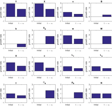
1.7 The two segments of the balanced growth path: annual growth rates before and after leisure-enhancing technological progress . . . 36
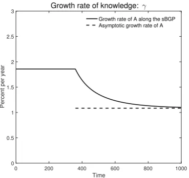
1.8 Growth rate of knowledge in the sBGP . . . 37
1.9 Some key variables on the sBGP . . . 37
1.10 Level of two measures of GDP on the sBGP . . . 38
1.11 Growth rates of GDP and productivity . . . 39
1.12 Planner’s objective as a function ofHLfor different values ofA, and the optimal allocation . . . 41
2.1 Capital-to-output ratio in the United States . . . 46
2.2 The unemployment rate and the labor share in the United States . . . 47
2.3 The task spectrum . . . 52
2.4 Demand for automation . . . 53
2.5 Stationary Equilibrium . . . 64
2.6 The stationary equilibrium vs. three benchmark economies . . . 65
2.7 Wage schedules under alternative bargaining protocols . . . 66
2.8 Price of manual goodsp¯in an unconstrained equilibrium. . . 70
2.9 Price of manual goods $\bar{p}$ in a constrained equilibrium. . . 72
2.10 Prices of tasks in the new equilibria . . . 75
2.11 Determination of the new stationary equilibrium . . . 75
2.12 Value of the job and underlying components across the two equilibria . . . 76
2.13 Decomposition of the change in the job value function between the two station-ary equilibria . . . 77
2.16 Arriving at a decomposition of the change in the wage across the asset
distribu-tion . . . 81
2.17 Dynamic path of the labor market following the rise in automation efficiency . 82 2.18 Transition path of the aggregate variables . . . 82
2.19 Transition of the distribution and the wage schedule . . . 83
2.20 Demand for assets with binding technological constraint . . . 83
2.21 Stationary equilibria that are technologically constrained . . . 84
2.22 Dynamic path of the labor market following the invention of new automation technologies . . . 85
2.23 Transition path of the aggregate variables following an increase inµ . . . 86
2.24 Dynamic path of wages across the distribution after an increase inµ . . . 86
2.25 Time evolution of total income quintiles . . . 87
3.1 Real interest rates estimated from the inflation-linked bonds and forward swaps 90 3.2 Changes in the equilibrium real interest rate as a result of policy, demographic and technological shifts . . . 93
3.3 Current account in advanced economy block and in selected individual economies . . . 95
3.4 Real returns in the United States: data and principal components . . . 96
3.5 AEs R* and trend growth . . . 100
3.6 Private saving and private investment: the level and gap . . . 101
3.7 Advanced economies government policy ratios (in proportion to GDP) . . . 102
3.8 Public social spending in the OECD . . . 103
3.9 Advanced economies R* adjusted for the impact of government debt . . . 109
3.10 Simulated impact of government policies on the equilibrium real interest rate in the life-cycle model . . . 116
3.11 Gini coefficient of disposable household income across the OECD . . . 122
3.12 Number of apps worldwide . . . 139
3.13 Free and paid apps offered in the Google Play Store . . . 139
3.14 R&D expenditure share of the (proxy for the) leisure economy . . . 140
3.15 Mobile phone use over the course of an average day . . . 141
3.16 Wage schedule in the SCF . . . 150
3.17 Fitted wage schedules across the years in the SCF . . . 151
3.18 Transition path of the labor market variables following an increase in µwhen the technological constraint is binding in the new equilibrium . . . 152
3.19 Transition path of the aggregate variables following an increase in µwhen the technological constraint is binding in the new equilibrium . . . 152
3.20 Panel regressions of R* and government debt . . . 155
3.21 Panel regressions of the z component of R* and government debt . . . 155
Chapter 1
Leisure-enhancing technological change
1.1
Introduction
In models of economic growth, technological change is an abstract generalization of a large and diverse set of innovations undertaken in the real world. What determines the success of these models is whether this generalization captures the essential features of the growth process. In this paper I distinguish between the familiar product- or process-innovations and inventions that areleisure-enhancing. I show that making this distinction helps us understand the salient patterns observed in the real world.
The defining difference between the two kinds of technologies is the way they are mone-tized. Improving a production process or introducing a new or higher-quality product tends to raise the profits of the innovator directly. Instead, leisure-enhancing innovations may sell below the cost of production (indeed, may be given away for free), bringing in little or no revenue. In-stead, these innovations are used to capture peoples’ time and attention, which are valuable and can ultimately be turned into profit. Some firms – such as platforms in the business of market-ing, advertising and brand building – need consumers’ time and attention in order to produce. Innovation efforts of these firms are thus focused on creating and improving services that com-plement leisure, in the hope that consumers recognize their attractiveness and spend more time enjoying them. This form of technological change makes leisure increasingly more attractive. The theoretical model developed in this paper traces out the implications of this phenomenon for the long-run equilibrium.
This paper attempts to make sense of three trends in the data. The first is that leisure-enhancing innovations have been around for a while and are now ubiquitous. The recently-constructed long-run data on the value of free content suggests that the leisure sector has been operating for some time (Figure 1.1).1 TV channels, websites, social media and free newspa-pers are all products that many people use every day. Businesses involved in supplying these services are hugely profitable and very large. As of March 2018, the top six of the world’s
1Measured at the cost of production, the value of free services has been relatively stable at about 1% of GDP
0 0.5 1 1.5 2
1929 1934 1939 1944 1949 1954 1959 1964 1969 1974 1979 1984 1989 1994 1999 2004 2009 2014 Print Audio-Visual Digital Combined
Percent of annual US GDP
Figure 1.1: Free ad-supported consumer content in the United States
Source: Nakamura, Samuels, and Soloveichik (2017). The figure shows the ratio of free consumer content, mea-sured by the costs of production, to GDP. Thus, for example, it does not capture a welfare measure of the value of Facebook, but only measure the cost of providing it.
20 30 40 50 60
1913 1929 1938 1950 1960 1970 1980 1990 2000 Australia Belgium Canada
Denmark France Germany Ireland Italy Netherlands Spain Sweden Switzerland United Kingdom United States
Hours per week
Figure 1.2: Trend growth rates of average hours worked in a range of advanced economies
Source: Huberman and Minns (2007). Note: Data refers to full-time production workers (male and female) in non-agricultural activities.
largest companies by market capitalization – Apple, Alphabet, Microsoft, Amazon, Facebook and Alibaba – are platforms whose business models, at least in part, rely on capturing peoples’ time and attention.
The second observation which this work speaks to is the decline in average hours worked and a corresponding rise in leisure hours. Figure 1.2 shows that, following the large falls in average hours worked at the start of the 20th century when the 5-day week became the norm, hours worked continued to decline also in the post-war period, by about 7 hours per week in the latter five decades of the last century.
Furthermore, there is suggestive evidence that changes in time allocation patterns may be linked to technology. Data that tracks how much time people spend on various electronic de-vices show a very rapid increase in recent years, largely due to widespread smartphone usage (Figure 1.3). This is true across many developed and developing economies.
0 2 4 6 8 10 12
2014 2015 2016 2017
Live TV DVR/Time-shifted TV
AM/FM Radio DVD/Blu-Ray Device
Game Console Multimedia Device
Internet on a PC App/Web on a Smartphone App/Web on a Tablet
Hours per day
Figure 1.3: Average time spent on media consumption per adult in the US
Source: Nielsen. Note: Figures for representative samples of total US population (whether or not have the technol-ogy). Data on TV and internet usage, and the usage of TV-connected devices are based on 248,095 individuals in 2016 and similar sample sizes in previous years. Data on radio are based on a sample of around 400,000 individu-als. There are approximately 9,000 smartphone and 1,300 tablet panelists in the U.S. across both iOS and Android smartphone devices.
seemingly rapid technological progress, productivity growth has been surprisingly weak across a wide range of advanced economies in recent decades (Figure 1.4) – what has come to be known asproductivity puzzle.
To elucidate how these trends are related, I develop a simple general equilibrium model with demand for and supply of leisure services and advertising. I start with a static model that helps to illustrate the novel mechanisms in a simple setting. I then add the dynamic choices and explore the implications of leisure-enhancing technologies for the balanced growth equilibrium. The static model has the following new features. Household leisure is defined as the utility generated from a range of activities, such as watching TV or browsing the web. To ‘generate’ leisure, households combine their time withleisure services(such as TV channels or web con-tent). To isolate the novel economic forces at play, the theory focuses on the services that are
free(available at zero price) andnon-rival(equivalently, once produced, there is zero marginal cost of supplying an extra user).2 Households value variety: the more leisure activities exist, the more attractive leisure is. On the firm side, households’ time is an essential input to the pro-duction of advertising, which is supplied to the rest of the economy by a marketing platform.3 Demand for advertising comes from producers of all other goods and services in the economy:
2In reality, some leisure services may sell at positive prices but below the cost of production. These products
can be thought of as a combination of the standard consumption good and leisure-enhancing products. The under-lying economic forces are similar; and the stark split in the theory developed here underscores the novel aspects of incentives driving innovation.
3I assume there is only one platform. One way to think about this assumption is as approximating a sector
-1 0 1 2 3 4 5
1960 1970 1980 1990 2000 2010
Labor productivity
Total factor productivity
Percent, 10-year annualised growth rates
Figure 1.4: Trend growth rates of total factor productivity and labor productivity in advanced economies
Source: Adler et al. (2017). Based on data from Penn World Table 9.0; IMF World Economic Outlook. The figure shows purchasing power parity GDP-weighted average for the largest 20 advanced economies.
each firm can shift its demand curve – sell more at any given price – by advertising its product. There are two main results that come out of the static setting. First, I show that in the static equilibrium there is positive supply of advertising and of leisure services as long as the economy is large enough. This is driven by the new kind of non-homotheticity: unless leisure is attractive enough, households choose zero leisure. In that sense, the model develops a microfoundation for when and why the leisure sector becomes viable. Second, the model highlights how GDP (as measured by statistical agencies worldwide) misses the value of leisure services when they do emerge. The size of this mismeasurement can be calculated and analyzed in equilibrium.
Embedding the model mechanisms in the dynamic setting brings out three further insights. First, leisure-enhancing technologies emerge endogenously in equilibrium once the econ-omy is sufficiently developed – a straightforward corollary of the result from the static setup that the economy must be large enough to feature leisure services in equilibrium. Thus the long-run equilibrium is characterized by what may be called asegmented balanced growth path
(sBGP).
Second, in presence of leisure-enhancing innovations, hours worked decline and leisure hours rise along the sBGP. From a theoretical standpoint, the model provides a novel way to embed falling hours worked in the long-run equilibrium. Empirically, this result matches the trend in time use observed across countries (Aguiar and Hurst, 2007b).
Third, TFP growth declines with the introduction of leisure-enhancing technologies. This is because more leisure translates into a slower growth rate of the pool of resources that are devoted to generating new ideas and knowledge. At the same time, traditionally-measured GDP struggles to capture the value of leisure services, potentially exaggerating the extent of the slowdown.4
4The present model abstracts from all other forms of leisure and focuses solely on leisure activities that are
The final set of results concerns the efficiency of the market equilibrium. The market equi-librium allocation involves two new inefficiencies which I uncover by studying the social plan-ner problem in the static and dynamic settings. In the static equilibrium there is undersupply of leisure technology, as the production of leisure services is governed solely by the prospective profitability of the marketing platform rather than on their true social value. In the dynamic model, there may be oversupply, precisely because of the adverse implications for the long-run growth rate.
Related literature. This study is related to several strands of literature. First and foremost, it builds on and contributes to the extensive literature on endogenous growth (Romer (1990), Aghion and Howitt (1992a), Jones (1995), Kortum (1997), Segerstrom (1998), Acemoglu and Guerrieri (2008), Ngai and Pissarides (2008), Aghion and Howitt (2009), Aghion, Akcigit, and Howitt (2014)). More specifically, it focuses on the ability of endogenous growth models to gen-erate balanced growth equilibrium in which hours worked decline over time, and in this sense it is closely related to the work of Boppart and Krusell (2016). The focus and the underlying eco-nomics differ substantially across the two papers, however: while Boppart and Krusell (2016) depart from the balanced growth preferences benchmark to develop the formulation consistent with declining hours and balanced growth (with the income effect stronger than the substitution effect), the theory in the present paper builds on balanced growth preferences and generates these outcomes endogenously in equilibrium.
The present paper draws on and contributes to the literature on the economics of time allo-cation. Starting from the seminal work of Becker (1965), economists have developed the theory of time allocation that is helpful in the analysis of the complementarities between consump-tion and leisure (recently summarized in Aguiar and Hurst (2016)). This paper is a first step in the direction of extending this literature to capture a salient features of the modern economy, namely, the rising supply of free and non-rival leisure-enhancing services.
The analysis of empirical evidence on time allocation patterns in recent years presented in the Appendix contributes to the literature that documents the changes in how people spend their time (with seminal contributions from Aguiar and Hurst (2007a) and Ramey and Francis (2009)). The focus on free leisure-enhancing services brings this paper close to the studies by Terranova (2012), Wallsten (2013) and Boik, Greenstein, and Prince (2016), all of whom consider the time and attention allocation problem in the context of the rise of the internet and digital technologies. Unlike these papers, the present study analyses this problem in a fully specified macroeconomic model, which allows for the study of both positive and normative macro implications. The focus on macroeconomic implications of leisure technologies brings the paper close to Aguiar, Bils, Charles, and Hurst (2017) who investigate how video games altered the supply of labor of young men in the United States. I cast the net more broadly, however, studying all leisure-enhancing technologies and highlighting the importance of the endogenous feedback mechanism between the innovations carried out by producers of these technologies and the resulting changes in the allocation of time and attention by consumers.
mea-surement, contributing to a large and fast-growing literature on the productivity puzzle and on measurement of the modern economy (Aghion, Jones, and Jones (2017)). In particular, the theory proposes a way to reconcile the two sides of the “productivity debate” by relating the rapid leisure-enhancing technological change to the lower rates of TFP growth.5 The model developed here suggests that in some sense both sides of this debate are correct: rapid techno-logical change in the leisure sector could well cause the growth rates of TFP to decline; thus the perception of rapid progress may well coincide with low observed TFP growth (Figure 1.4). Furthermore, the model allows for a clean analysis of different measures of activity, depending on whether and how one values the leisure services. It contributes to the literature on mea-surement challenges, particularly those that arise when goods and services are provided at zero prices (Bean (2016), Bridgman (2016), Syverson (2016), Brynjolfsson, Eggers, and Ganna-maneni (2017), Byrne, Fernald, and Reinsdorf (2016), Nakamura, Samuels, and Soloveichik (2017), among others).
Finally, this paper builds on several literatures in industrial organization which study two-sided markets and economics of advertising. Classic references on the economics of platforms are Rochet and Tirole (2003) and Anderson and Renault (2006) who study the equilibrium pricing decisions in two-sided markets. More recently, Tirole (2017) provides a non-technical overview of the major forces at play, and highlights the rising importance of the platform busi-ness model in the modern economy. There is an extensive literature on the economics of ad-vertising, going back to Marshall (1890) and Chamberlin (1933), and summarized in the IO Handbook Chapter by Bagwell (2007). More recent research has considered the effectiveness of advertising in the context of modern technologies (DellaVigna and Gentzkow (2010), Lewis and Reiley (2014), Lewis and Rao (2015)). The present paper contributes to these literatures by analyzing platforms in a general equilibrium setting and drawing out the implications within a canonical macroeconomic model of competition and growth.
Roadmap. The remainder of this paper is structured as follows. Section 1.2 lays out the static model and derives the main optimality conditions. Section 1.3 shows how these conditions can be adapted to a dynamic endogenous growth setting, defines and characterizes the balanced growth equilibrium. Section 1.4 discusses the welfare properties of the market equilibrium. Section 3.7 concludes and suggests areas for future work.
5“Productivity optimists” build their case with anecdotes of groundbreaking technological innovations,
Households Marketing
platform
Consumer goods producers Retail firms
Leisure time, data
Leisure services
$
ad
s
F
in
al
go
o
d
L
ab
o
r
$
$
Consumption goods
Figure 1.5: The model structure
1.2
The static model
The model builds on the standard framework of monopolistic competition (Dixit and Stiglitz, 1977). Figure 1.5 illustrates the basic structure, with the “leisure sector” highlighted in red. In the reminder of this Section I present a detailed outline of the economy and derive some initial results.
1.2.1
Household’s time allocation problem
The economy is populated by two kinds of households: workers and capitalists. Capitalists do not work; they own all firms in the economy and finance hand-to-mouth consumption with the flow of corporate profits.6
In a static setting, there is a unit-measure of working households. Households have separa-ble utility over consumption and leisure. Specifically, I work with a canonical form of balanced growth preferences, as in King, Plosser, and Rebelo (1988) and (2002), with log utility from consumption and a constant-elasticity power utility of leisure (see also Boppart and Krusell (2016)). I allow for the possibility that there are network effects in leisure, external to individ-ual choices, which is a plausible feature of some of the modern leisure services such as social media. The instantaneous utility function is:
upc, lq “logpcq ` l 1´ξ
1´ξ ¨fp
¯
HLq (1.1)
wherelis leisure andfpH¯Lqis an increasing function that takes as argument the average hours
spent on leisure, denoted by H¯L. I further assume that0 ď ξ ă 1, which implies that utility
is weakly concave in leisure (ξ ě 0) but that the curvature is not too extreme (ξ ă 1). This ensures that leisure-enhancing innovations raise leisure time.7
6This removes the profit flow from the working households budget constraint which allows for a closed-form
solution to the model. I denote aggregate consumption of capitalistsC.
7As highlighted in Section 2, the evidence suggests that leisure-enhancing technologies indeed raises the total
In a workhorse macro model of labor supply, leisure and leisure time are one and the same thing. Here I instead view leisure as utility that comes from spending time on a range of leisure activities of measureM:
l“
¨
˚ ˝
M
ż
0
rminthpjq, mpjqus
loooooooooomoooooooooon
activitypjq
ν´1
ν dj
˛
‹ ‚
ν ν´1
. (1.2)
In this expression activities are indexed byj, andhpjqis the time spent on activityj andmpjq
denotes leisure services required for this activity. Parameterν is the elasticity of substitution across different activities, and is assumed to be greater than unity:ν ą1.
Several assumptions are embodied in this formulation. First, the assumption that the elastic-ityν is greater than 1 implies that different activities are imperfect substitutes: there islove for varietyin preferences, in the sense that, all else equal, more varieties yield higher leisure util-ity. Second, to generate leisure, each activity requires both time and leisure services, and only those. Thus the formulation assumes away any potential complementarities with consumption.8 Finally, there is no substitutability between time and free services: enjoying a favorite TV show or surfing the net necessarily requires free time in fixed proportion. This assumption is a natural in the context of services that are available free of charge. Allowing for some substitutability between leisure services and leisure time would make the problem ill-defined.
The household chooses how to allocate their time across activities, leading to the result summarized in the following Lemma:
Lemma 1 Given (1.2), individuals’ optimal allocation of time across available leisure varieties implies that the leisure production function is linear in total leisure time:
l “HLM
1
ν´1. (1.3)
The simple proof is in the Appendix. The key step is to note that, given that servicesmpjqare free of charge and are non-rival, household is never constrained bympjq.
Equation (1.3) says that for a given amount of leisure time, leisure utility increases in M. This love for variety effect vanishes as ν Ñ 8: if different varieties of leisure are perfectly substitutable, only the total time spent on leisure matters and the number of activities become irrelevant.
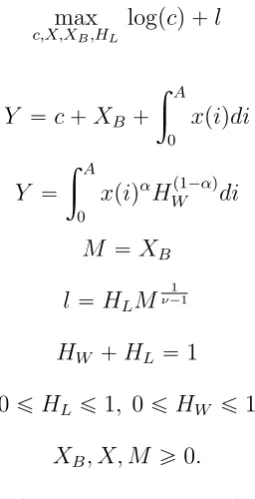
The problem of choosing the optimal labor supply can be written in the following way:
max
c,HL
logpcq ` l 1´ξ
1´ξ ¨fp
¯
HLq
8Conceptually, there are several kinds of inputs that may feature in leisure production: (i) time; (ii)
subject to:
l “HLM
1
ν´1, c“w¨H
W, HW `HL “1, HW ě0, HLě0,
whereHW denotes time spent working, and time endowment is normalized to 1.9
Focusing on the interior solution, the first order condition then implies:
1
HW
“HL´ξM1ν´´ξ1fpH¯
Lq. (1.4)
Because the time endowment constraint implies that HW “ 1´HL, and in equilibrium
HL “ H¯L, equation (1.4) pins down the optimal choice of leisure hours HL˚ , which is an
increasing function ofM. It is then straightforward to find a solution for all other variables of interest, such as labor supplyH˚
W and consumptionc˚.
Implications for balanced growth. This characterization of the static equilibrium carries implications for the dynamic model I study in Section (1.3). The key one is that, without fur-ther restrictions, optimality condition (1.4) isnotconsistent with balanced growth in a dynamic setting if M changes over time. To see this, suppose that M grows at some constant net rate γM.It is easy to see that the optimal labor supply changes with M. For balanced growth we
usually require that hours worked are constant; but in principle there exists another possibility, which is that hours worked decline at a constant rate:γH ď0.10 On such a path, hours decline
asymptotically towards zero, and leisure hours increase at anon-constantrate.11 This is incon-sistent with condition (1.4), however, because this condition implies that under the hypothesis of constant growth rates ofM andHW,the growth rate of leisure hours is constant too.
Additional assumptions on the functional form of the utility function need to be imposed to ensure balanced growth. These requirements are contained in the following Proposition: Proposition 2 Consider a dynamic environment in which household preferences are described by the instantaneous utility function in (1.1), in which the number of leisure varietiesM grows at a constant rate in equilibrium. A balanced growth equilibrium with hours worked decreasing
at a constant rate is consistent with these preferences under either of the two conditions:
Condition 1. ξ “ 0; that is, utility is linear in leisure, andfpH¯Lq “ 1,that is, there is no network effect; or
Condition 2. The network effect takes the form of a power function with exponent equal to
ξ: fpH¯Lq “H¯Lξ.
9Clearly, this formulation focuses only on marketable leisure, abstracting from other uses of time, such as
home production, non-marketable leisure, or sleeping.
10Note that this is the only other possibility: for example, leisure hours rising at a constant rate would imply
zero hours worked at finite horizon, which would yield zero consumption, an outcome clearly inconsistent with utility maximization.
11To see this mathematically, note that ifxptq `yptq “constant, taking logs of both sides and differentiating
the time constraint with respect to time yields: x`1y
´
dxptq
dt `
dyptq
dt ¯
“0 . The expression on the left hand side
can be rewritten as x`xydxdtptq1x` x`yydydtptq1y “ x`xyγx`x`yyγy whereγdenotes net growth rate of a variable,
which itself is, in general, a function of time. Setting this equal to zero, the two growth rates satisfyγy “ ´xyγx.
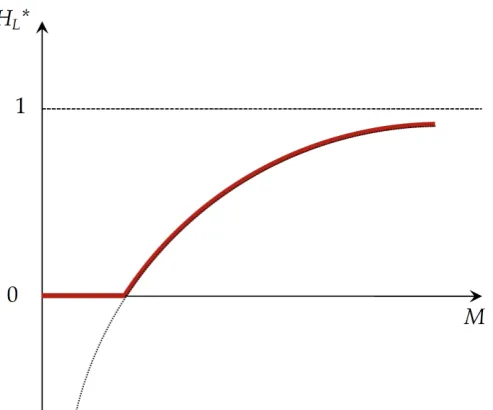
Figure 1.6: Optimal choice of leisure hours as a function ofM
Proof. Both of these conditions eliminate the dependence of the right hand side of (1.4) from HL, implying thatHW “M
1´ξ
ν´1. Thus ifM grows at a constant rate, hours worked can grow at a constant rate with no further restrictions on the growth rate of leisure hours. In the remainder of the paper I assume that Condition 1 of Proposition 2 holds.12 Under these assumptions, the optimal choice of leisure hours is given by:
H˚
L“maxt0,1´M
1
1´νu. (1.5)
The key result is that, for M sufficiently large, optimal leisure hours depend positively on the measure of available leisure options. The generic shape of the leisure supply function is depicted in Figure (1.6). Because households like variety, more abundant leisure options make leisure more attractive relative to work, and households optimally choose to work less and play more. There is, however, the possibility of the corner solution: for smallM, the optimal choice of leisure hours is zero.
1.2.2
Demand for advertising
The competitive retail sector produces final output by combining labour with a continuum of consumer products xpiq indexed from 0 to A. The key is that the share of each product in the mix is affected by the relative advertising spending of each produceri. In particular, the final good is produced according to the following constant returns to scale aggregate production function:
12Thus, to simplify the notation and the algebra, in the remainder of the paper I assume thatξ
Y “
A
ż
0
˜ ˆ
bpiq
¯
B ˙χ¨O
xpiq
¸α L1´α
Y di (1.6)
wherexpiqare the individual consumer varieties, andLY is labour employed in the retail sector.
The term ´
bpiq ¯ B
¯χ¨O
guides how advertising enters the model. Here,bpi) is firmi’s ad spending andB¯is the average marketing expenditure across all producers:B¯ ” A1 ş0Abpiqdi. The fraction
bpiq ¯
B measures the relative advantage of firm i due to its marketing efforts as compared to its
competitors.13 Parameter χ ě 0 measures firms’ perceptions of the sensitivity of demand for their product to advertising efforts: the value of zero corresponds to the situation where indi-vidual firms view advertising as useless, and the model collapses to the standard monopolistic competition setting found in the literature. Finally,O is a binaryt0,1uvariable which denotes the choice of the marketing platform whether to operate or not (discussed below).
The implication of equation (1.6) is that only by advertising more than its competitors can a firm boost demand for its product: marketing is all aboutrelative advantage. This is consis-tent with wealth of empirical evidence, summarized in Bagwell (2007): while advertising may have significant impact on any individual firm’s sales, the effect disappears once the unit of observation is expanded to a sector or the macroeconomy.
The present model is silent on the channels through which advertising operates, and assumes there is no direct utility impact of advertising. The literature highlights three reasons why adver-tising may work: providing information, persuasion, and complementarity with consumption. In this paper I take it as given that advertising efforts shift relative demand, but do not take a stance on the channels through which this operates. In the same vein, I assume that ads do not affect household’s welfare directly: one possible interpretation is that the positive information effects broadly offset the negative utility impact associated with exposure to ads. None of the positive economics of what follows is affected by this assumption.
Differentiated goods are produced by a continuum of monopolistically competitive firms indexed byi. For simplicity, I assume that each firm has access to a technology that converts one unit of final output into one unit of consumer good: xpiq “ X,whereX is the amount of final good used in the production of goodi. Each firm faces a demand curve for its product, and each has the option to spend resourcesbpiqon advertising, a service provided by the marketing firm at a given pricepB. Any individual produceritakes the average level of advertising B¯ in
the economy as given.
13The retail sector anticipates any shifts in relative demand due to firms’ marketing efforts and demands more
1.2.3
The marketing platform
The marketing platform simultaneously operates along two margins: it supplies advertising to businesses, and produces varieties of leisure services. The latter is necessary to operational-ize the former, because peoples’ time and attention are required inputs in the production of advertising.
This structure of the business poses interesting problems for optimal pricing and production strategies, a subject of the literature in industrial organization. Classic papers by Rochet and Tirole (2003) and Armstrong (2006) and the recent book by Tirole (2017) conclude that the equilibrium pricing structures depend on the elasticities of demand on both sides of the market as well as on externalities between two groups of customers. If one side of the market benefits substantially more than the other from the interaction, then that side will be charged more, including the possibility that the other side may not pay anything.
In practice, many leisure services are indeed provided free of charge to the consumers (Fig-ures 1.1 and 3.13 provide some indication). This equilibrium pricing configuration appears to be prevalent in the leisure sector, perhaps because the interaction between consumers of leisure services (people) and consumers of advertising (firms) directly benefits the latter. The consumer side ends up being the “loss leader”, while the business side is where the revenue is generated. While the full analysis of these pricing strategies is beyond the scope of this paper, armed with the logic of economic forces identified in the literature, I assume that the platform chooses to charge a positive price only to the business side. Thus the problem of the platform is to choose whether or not to operate, and to maximize profits by optimally choosing the price of advertising pB.This choice will then imply the optimal supply of advertising and of leisure services.
The platform is characterized by two technologies and two constraints. The constraints are the household’s leisure supply schedule and the firms’ demand for advertising.14 I make the following assumptions with regards to the technologies:
1. Production function for the number of varieties is linear in final good used by the platform, XB:
M “XB; (1.7)
2. Household leisure time is the only input required to produce marketing, and the produc-tion funcproduc-tion takes the following funcproduc-tional form if the platform chooses to enterpO “1q:
B “
$ &
%
0 if HL “0 1
1´HL if HL ą0
, (1.8)
andB “0otherwise. HereB is total marketing sector output.
These are strong assumptions and they merit further discussion. Assumption (1) is driven by the desire for parsimony: the linear one-to-one technology is perhaps the simplest possible
14The former was derived above, the latter can be easily obtained by solving firm i optimization problem:
pB “α
2 1´αχ 1
bpiq
´
bpiq
¯
B ¯1´ααχ
formulation. Note that production function forM reflects the fact that servicesmpjqare non-rival. Production of an extra variety of leisure - increasingM - requires real effort and resources; but once a specific varietyj has been produced, it provides unlimited amount of servicesmpjq
within a period. AllM varieties are perishable, in thatM is modeled as a flow and not a stock. These simplifying assumptions stand for a more general idea that the marketing firm spends resources on improving leisure options of the consumer. Future work could usefully explore different ways of modeling M and the process of technological improvements of the leisure options.15
Formulation (2) consists of a set of assumptions, with varying degrees of importance. The most fundamental one is that HL is an input into the production for marketing, which makes
leisure time a valuable commodity in this economy. To provide advertising, the platform must attract “eyeballs”.
Second, it assumes that there are increasing returns to scalein the production of advertis-ing content. This is a necessary feature for the model to be consistent with balanced growth, where one of the factors of production is bounded (in this case,HLď1). This ensures that the
marketing platform is able to produce arbitrarily large amounts of advertising servicesB as the economy grows indefinitely. One justification for a convex production function is that, at higher levels ofHL, the marketing firm is better able to learn about consumers’ tastes and preferences,
and thus to provide more targeted advertising. Arguably, such information acquisition appears to play an increasingly important role in the real world, and increasing returns is a simple way to capture this force. This assumption is not without controversy, however. The marginal effec-tiveness of advertising may decline as the cognitive and memory limits start to bite, suggesting that decreasing returns may be a more plausible alternative. Without convexity, there will be a limit on the size of the marketing sector, and at some point along the growth path advertising prices will rise rapidly as demand outstrips supply.
Furthermore, some of the technical constraints faced by firms in this sector suggest that decreasing returns may be a better assumption. For example, the success of machine learning techniques used for targeting consumers’ behavior depends on the accuracy of their predictions. But the prediction accuracy increases with a square-root of the number of observations (Varian (2017)), which is a hard, statistics-driven constraint on the growth potential of leisure platforms. All in all, the assumption of increasing returns imposed here should be interpreted as one that is necessary for the economy to admit a balanced growth path. The sheer size and profitabil-ity of the largest platforms suggests that the assumption of increasing returns is a useful one to describe the past experience. The validity of this assumption going forward is an interesting area for future work.
Equation 1.8 makes it possible to solve the problem in closed form. Combining (1.7) and (1.8) yields a quasi-production function that consolidates the platform technologies:
15One possibility is that the leisure time itself is an important part of the production process of leisure varieties
B “X
1
ν´1
B . (1.9)
Equation (1.9) reveals that the set of assumptions discussed above implies that the produc-tion funcproduc-tion of the platform is a simple, smooth and concave neoclassical producproduc-tion funcproduc-tion with diminishing marginal productivity in the final-good input. This implication facilitates a closed-form solution to the model.
1.2.4
Equilibrium in the static model
1.2.4.1 Definition of market equilibrium
Definition 3 The market equilibrium in this economy is a set of aggregate quantities tc, C, Y, B,B, M, X, X¯ B,ΠB, HW, HL, LYu, individual-variety quantities
tmpjq, hpjq, xpiq, bpiq,Πpiqujj,i““M,i0 “A, and pricestw, pB, qpiquAi“0 such that:
• Working households maximize utility subject to the budget constraint and the time en-dowment constraint, taking wageswand the number of leisure optionsM as given; • The retail sector maximizes profit, taking wages w, prices of the consumer sector goods
tqpiquAi“1, and advertising spendingtbpiquAi“1as given;
• Each producer i chooses quantity xpiq, price qpiq and the advertising expenditure bpiq
to maximize profits, subject to demand curve for their product and taking the average advertising spending in the economyB¯as given;
• The marketing platform sets the price of advertising services pB, supplies quantities
tbpiquAi“1,and produces M varieties of free services to maximize profits, taking as given
the average level of ad spendingB.¯ • Capitalists consume all profit income;
• Goods market clears: Y “c`C`X`XB;
• Labour market clears: LY “HW.
1.2.4.2 Characterization of the equilibrium
I solve the model under the assumption that the platform finds it worthwhile to be active:O “1. I then derive the conditions under which this is indeed the platform’s optimal choice.
The retail sector.The maximization problem of the retailer is:
max
xpiq,LY A
ż
0
ˆˆ bpiq
¯
B ˙χ
xpiq
˙α L1´α
Y di´ A
ż
0
xpiqqpiqdi´wLY (1.10)
α ˆ
bpiq
¯
B ˙αχ
xpiqα´1LY1´α “qpiq (1.11)
whereqpiq is the price of variety i of the consumer good. Equation (1.11) shows that higher advertising expenditures of produceri, holding advertising of all other firms constant, shifts the demand curve out (for any given priceqpiq, firmican sell a higher quantity of its product).
Consumer sector. Intermediate producers maximize profit, subject to the linear technology (recall thatxpiq “X) and demand curve in (1.11). Each firm can also buy advertising at a given pricepB. In effect, the problem of each producer is:
max
xpiq,bpiq
α ˆ
bpiq
¯
B ˙
αχ
xpiqαL1´α
Y ´xpiq ´pBbpiq. (1.12)
The first order conditions to this problem yield the standard result that, for each producer, price equals mark-up over marginal cost (qpiq “ q “ α1). They also give the inverse demand curve for marketing:
pB“α
2 1´αχ 1
bpiq
ˆ bpiq
¯
B ˙1α
´αχ
LY. (1.13)
Marketing platform. The platform chooses the quantity of advertising supplied to maxi-mize profits, subject to the demand curve for marketing services (1.13) and to the consolidated production function (1.9). This maximization problem can be written as follows:
max
bpiq
żA
0
α1´2αχ
ˆ bpiq
¯
B ˙1α
´αχ
LYdi´
ˆżA
0
bpiqdi ˙ν´1
Optimality and the symmetry of the problem imply that, in equilibrium:
B “ pκALYq
1
ν´1 (1.14)
whereκ “ 1´ααχ2α
2 1´αp 1
ν´1qis a constant. Next, combining (1.14) and (1.9) gives the
expres-sion for the inputs used by the platform:
XB “κALY. (1.15)
Finally, note the labour market clearing implies that:
LY “HW “X
1 1´ν
B (1.16)
where the last equality follows from household optimization under the assumption that market-ing sector is active. Combinmarket-ing (1.15) and (1.16) gives the expressions for equilibrium levels of final output used in production of advertisingXB and total advertising outputB as function of
the exogenous parameters of the model:
XB “ pκAq ν´1
B “ pκAq
1
ν. (1.18)
Unsurprisingly, the equilibrium size of the marketing platform depends positively on the measure of varieties: the more goods varieties there are, the higher the demand for advertising. Marketing firm is also larger for higherχand lowerν.A higherχmeans that individual firms believe advertising is a powerful way through which one may increase profits, and a lowerν means that the link between the leisure-technology and leisure supply is stronger.
This structure implies the following Lemma:
Lemma 4 The platform has a minimum scale of operation. It is active (O “ 1) if and only if
M˚ “X˚
Bě1, whereM˚ andXB˚ are the optimal choices of the monopolist.
The Lemma follows from the production functions forM andBin (1.7) and (1.8), respectively, and from the household’s leisure supply (1.5): since the household allocates no proportion of their time to leisure ifM ď1, it follows that the platform can produce positive levels ofB only whenM ě1.
Given (1.9), it follows that the sufficient conditions for the platform to be active are that: (i) its equilibrium output is greater than one (B˚
ą1) and (ii) that its profits are non-negative. The latter is simply a restriction on the parameters of the model which I assume is satisfied.16 The following Proposition characterizes the former:
Proposition 5 The marketing sector is active only in an economy that is large enough. In particular, the condition for the emergence of the marketing sector is given by:
Aą 1
κ. (1.19)
If the economy is small, and the above condition is not met, the marketing sector remains
inactive, withO “0. In that case the structure of equilibrium is identical to a standard model of monopolistic competition. If (1.19) holds, the marketing sector is active and the scale of its
operations in equilibrium is given by (1.18).
Proof. The result follows immediately from equation (1.17) and Lemma 4. The result that the economy collapses to a standard model when the marketing firm is inactive follows immediately from settingO equal to zero in (1.6) and noting that forM “ 0households’ labour supply is inelastic.
Intuitively, when the number of product varieties is small, there is little profit to be made from supplying marketing services. Relative to these limited profit opportunities, the marketing platform finds it too costly to produce enough of the leisure varietiesM to get the households to spend any time on leisure.
16Marketing platform profits areΠ
B “ pα
2
1´αχ´κqALY, which is positive if and only if α
1´αχ
1
ν´1 ă1. I
1.2.4.3 GDP in the model and in the data
Is GDP as currently measured in the data a useful metric for activity in the modern economy? To begin thinking about this issue, is useful to review how the activity of the marketing sector is measured in the data at the moment. Bean (2016) concisely describes the current practice:
Most of the web’s popular destinations, such as Google, Facebook, and YouTube, rely on advertising to generate income. [...] Digital products and services are ef-fectively paid for by the advertisers. As such, the 2008 UN System of National Accounts (SNA) treats them as an intermediate input in the advertising industry. Therefore, the advertisement expenditure adds to the value added of the industries supplying advertisement space, and at the same time detracts from the value added of the advertising industries. Consequently the value of digital products nuanced through selling advertising space will be accounted for in aggregate GDP only to the extent that it also translates into higher consumption of the goods and services being advertised.
In our model, advertising is a beggar-thy-competitor, zero-sum activity: there is no increase in consumption that results from it in equilibrium. Consequently, it is clear that GDP, the way it is measured in the data, would not capture any of the value generated by the marketing sector.
To be more specific, consider the true measure of GDP in the context of the present model, denoted byGDPmodel. It is a sum of gross output in each sector: the retail sector (Y), consumer
sector (ş0Axpiqdi), advertising firm (BandşM0 mpjqdj), less the value of the inputs used in these
production processes.17 The key challenge is to measure the value of leisure services. One way to do so is to rely on current wages that reflect the opportunity cost of time (Goolsbee and Klenow (2006), Brynjolfsson and Oh (2012)). This leads to a valuation method where the value of these services is set to equal the time spent on them, evaluated at the current wage rate. In light of the equilibrium conditions above, the value of these services is thus:
w¨
M
ż
0
mpiqdi “w¨
M
ż
0
hpiqdi“wHL“w¨
˜
1´
ˆ
1
κA ˙ν1¸
“ p1´αqα
2α
1´αA
˜
1´
ˆ
1
κA ˙1ν¸
.
Taking this methodology of valuing leisure services as given, the equilibrium GDP in this economy can be expressed a function of the primitives of the model:
GDPmodel“κ´
1
νA ν´1
ν
„ α1´2α
ˆ
1
α2 ´1
˙
´κ
looooooooooooooooooomooooooooooooooooooon
GDPmeasured
` p1´αqα12´ααA
« 1´ ˆ 1 κA ˙1 ν ff loooooooooooooooooomoooooooooooooooooon
V alue of leisure services
.
True GDP is a sum of two components: the measure of activity of the “traditional” sector, which is properly captured by statistics agencies, and the value of leisure services. For any set
17Derivations of gross outputs of each sector and the verification of the goods market clearing condition are in
of parameters, the model allows for a precise analysis of the degree of mismeasurement. This is particularly interesting in dynamic model, to which I now turn.18
1.3
Dynamic model
There are three key features of the dynamic model relative to the static setup above. First, there is the R&D sector, which employs researchers to invent new varieties of consumption goods. The size of the economy – measured as the number of varietiesA– is no longer a parameter; instead, it is endogenously determined by the optimal choices of the firms in the R&D sector. Second, households now solve an intertemporal consumption-saving problem. Third, there is population growth, and agents can be employed in the final goods sector as well as in R&D, which alters the labor market clearing condition.
1.3.1
The R&D sector
Time is continuous. New varieties of differentiated goods are invented by the R&D sector employing researchers. I follow Jones (1995) and propose a general formulation of the ideas production function, with the possibility that there are externalities from the stock of ideas over time (represented byφ ă1), and that there may be diminishing returns to employing researchers (represented by0ăλ ď1):
9
Aptq “ζAptqφLAptqλ. (1.20)
Given this technology, R&D producers choose how much labour to employ in order to maximize profits:
max
LA 9
AptqPAptq ´wptqLAptq
wherePAis the price of a patent which gives the holder of the patent a perpetual right to produce
that particular variety. The first order condition of this problem is:
PAptq “
wptq
ζAptqφLAptqλ´1
. (1.21)
A consumer firm is willing to purchase a patent as long as the return from doing so exceeds the required rate of return on investment,r, meaning that the following no arbitrage condition
18An alternative way of incorporating the zero services into the measured GDP is to consider the production
holds in equilibrium:
Πptq
PAptq
`
9
PAptq
PAptq
“rptq (1.22)
This condition has a standard interpretation: the flow return of purchasing a patent (the dividend plus the capital gain) must equal the rate of interest.19
1.3.2
Decentralized equilibrium
To save on notation, I drop time subscripts when defining the decentralized equilibrium. Definition 6 In light of the previous equations, a dynamic market equilibrium is a set of paths of: aggregate quantities:tc, C, X, XB, HW, HL, LA, LY, A, M, Bu8t“0; quantities of individual varieties:txpiq, bpiq, mpjq, hpjqu8iPA,jPM;t“0; prices of each intermediate input and of marketing services: tqpiq, pBu8iPAt,t“0; interest rates and wages: tw, ru8t“0; marketing platform activity indicator:tOu8t“0; such that:
• Working households maximize utility subject to the law of motion for per-capita assets, the leisure production technology, and the no-Ponzi game condition, taking as given all prices and the number of available leisure options;
• Capitalist households consume firms’ profits every period;
• Retail sector firms maximize profit taking prices and advertising spending of each variety as given;
• Intermediate goods producers maximize profits subject to the technology of production and demand curve for their product, taking as given the average level of advertising in the economy;
• The marketing platform maximizes profits subject to the marketing production technol-ogy, leisure varieties production technoltechnol-ogy, households’ optimal time allocation deci-sions, and the demand curve for marketing services. It becomes active only if it can be profitable.
• The R&D producers maximize profits subject to the ideas production function and the free entry condition.
• Labour market and goods market clear. I now characterize the equilibrium allocation.
19Note that the price of a patent grows at the same rate as population: PA9
PA “n. To see this, note that the price
of a patent will reflect the stream of profits generated by varietyi, discounted by the effective discount rate, which will be the market interest raterminus growth rate of populationn:
PA“
8
ż
t
e´pr´nqsΠds
“ Π
r´n
1.3.3
Household intertemporal problem
The standard household problem yields the Euler Equation and the intratemporal optimality condition (the Appendix contains the full derivation):
9
cptq
cptq “rptq ´ρ; (1.23)
wptq
cptq “Mptq
1
ν´1. (1.24)
1.3.4
Condition for the marketing sector to be active
To determine whether or not the marketing platform is active, it is useful at this point to derive a dynamic equivalent of the condition in Proposition 5. The condition differs from the one in the static setting because the labour market clearing condition is different: workers are now employed both in the retail and in the R&D sectors and population is growing over time. Labour employed by the retail sector is now:
LYptq “HWptqp1´sptqqNptq (1.25)
wheresis the share of the workforce employed in the R&D sector (which will be asymptotically constant in the balanced growth equilibrium). Equation (1.25) is simply an accounting identity which states that total labour supply in the final goods sector is equal to average hours worked times the number of workers employed in the retail sector.
Equations (1.15), (1.16) and (1.25) imply that in the dynamic setting the optimal choice of XB is given by:
XBptq “ pκp1´sptqqAptqNptqq ν´1
ν . (1.26)
We thus have the following Proposition:
Proposition 7 In a dynamic economy, the platform is active and there is leisure-enhancing technological change if and only if
Aptq ¨ p1´sptqq ¨Nptq ą 1
κ. (1.27)
Proof. The Proposition follows from combining equation (1.26) with the fact that, for the marketing sector to be active, we must haveXB ą1.
1.3.5
Segmented Balanced Growth Path
Given the result in Proposition 7, the balanced growth equilibrium in this economy is defined as follows:
Definition 8 A segmented balanced growth path (sBGP) is an equilibrium trajectory along which: (i) when (1.27) is not satisfied, per capita consumption, output and the measure of
varietiesA all grow at a constant rate; (ii) ast Ñ 8, per capita consumption, output,Aand
M grow at possibly distinct but constant rates, and average hours HW decrease at a constant rate.
The segmented Balanced Growth Path is then characterized by the following Proposition: Proposition 9 Characterization of the sBGP.
There existsˆtsuch that (1.27) holds@těˆt.
For t ď ˆt, average hours worked are constant pHW “ 1q, and per capita consumption, output, wages and knowledge all grow at the same constant rate given by:
gc “gy “gw “gA “
λn
1´φ. (1.28)
Fortěˆt, the marketing platform is active and the economy transitions to the other segment of the sBGP. AstÑ 8, average hours worked decline at a constant rateγH “ ´1νpγ`nqand the growth rate ofAis lower thangA. Specifically, it is given by:
γ “ nλ
`ν´1
ν
˘
1´φ``λν˘. (1.29)
Proof.The first part of the Proposition follows from the fact that the left hand side of (1.27) is a growing quantity (as there is positive population growth) while the right hand side is a constant. Consider the section of the BGP where the condition (1.19) does not hold. This implies that the platform is inactive:O “0. It is then straightforward to see that the economy is identical to the model economy studied in Jones (1995). In that economy, the measure of consumer goods varietiesA, wages, output and consumption per capita all grow at the same constant rate given by (1.28). The proof is available in Jones (1995) and is omitted for brevity.
To prove the final part of the proposition, note first that the solution to the household’s in-tratemporal optimization problem implies that average hours worked are a power function of the number of leisure varieties (recall equation (1.5)). Thus the growth rate of average hours must be proportional to the growth rate of varieties of leisure if the two variables grow at constant rates, so that:20
γH “
1
1´νγM (1.30)
20Note that, for variablesX andY, ifY
“Xathen gross growth rates satisfyζ
Y “ζXa and net growth rates
Next, equation (1.7) implies that theM andXBgrow at the same rate in equilibrium. Equation
(1.26) implies that this rate is given by:
γXB “γM “
ν´1
ν pγ`nq (1.31)
whereγ is the net growth rate ofA. Combining (1.31) and (1.32) gives the expression for the growth rate of average hours worked as a function ofγ:
γH “ ´
1
νpγ`nq (1.32)
Next, note thatγis, by definition, given by:
γ ”
9
Aptq
Aptq “
ζLAptqλ
Aptq1´φ (1.33)
On the segmented balanced growth path, the left-hand side of this equation is asymptotically constant by definition. That means that the numerator and the denominator of the fraction on the right-hand side must grow at the same rate. More formally, using the fact thatLA“HW¨N¨s,
differentiating (1.33) with respect to time gives and solving forγ yields:
γ “ λpγH `nq
1´φ (1.34)
Together, the two relationships, (1.32) and (1.34), are two equations in two endogenous vari-ables that readily give the expression forγ in equilibrium. The fact thatγ ăgAfollows
imme-diately from the comparison of the two expressions.21,22
Discussion. Proposition 9 contains several key results which I now discuss.
First, it tells us that the economy transitions endogenously from one segment of the BGP to another, when condition (1.27) is first satisfied. Fundamentally, this is driven by the juxtapo-sition of the household leisure supply, which is zero for low values ofM, and the fact that the platform requires some of household’s time to produce. The theory highlights the importance of market size (and the associated strength of demand for advertising) as the key force behind the emergence of the marketing sector.
To be sure, in reality there are other reasons, absent from the parsimonious model presented above, for why leisure-enhancing technological change emerges in equilibrium. For example, the invention of the washing machine and other appliances dramatically cut the time required to complete the necessary household duties, which meant that households had more time to allocate to other activities, including leisure. This meant that the potential market for leisure services expanded, which could have directed innovations towards the leisure sector, as in the
21The associated rate of decline of average hours worked is given byγ
H“ ´1ν
„
λnpν´1
ν q
1´φ`pλ
νq
`n
which goes to
zero asν Ñ 8.
22Finally, it remains to check that utility is bounded on the sBGP. This is indeed the case for a discount rate that
directed technical change literature (Acemoglu (2002)). More recently, other technological breakthroughs notably the invention of the internet and the subsequent hardware advances -opened up new possibilities to reach people’s consciousness throughout their day (recall Figure 3.15), amass large quantities of data, and target advertising with extraordinary precision. The theory presented here, while falling short of modeling these forces explicitly, is not contesting their importance. Instead, it is complementing these well-known explanations with a new one that might have previously been overlooked.
Second, the balanced growth equilibrium features declining hours worked. This is a unique feature of the theory developed here: the model matches (at least qualitatively) the key trend observed in the data without the need to hardwire the decline in hours into household prefer-ences, and shows that despite this trend, growth can be balanced, in the sense that all variables of interest grow at constant rates. In a standard model with endogenous labor supply, falling hours worked on the balanced growth path can be ruled as violating household intratemporal condition in finite time. Here, instead, this very intratemporal choice is the key force driving the downward trend. Furthermore, the model stresses the importance of innovation that is targeted specifically at capturing people’s time, a mechanism that is arguably at the heart of the modern economy but is new to macroeconomic models.
The third result is that TFP growth slows down as the leisure sector emerges. What is the intuition behind the decline in TFP and does it make sense? In the class of semi-endogenous growth models (to which the present model belongs), such as Jones (1995), Kortum (1997) and Segerstrom (1998) models, the long-run growth rate is determined by the growth rate of the total pool of resources that can be used to generate ideas. Bloom, Jones, Reenen, and Webb (2017) highlight that this is the relevant framework to think about growth, because of the key observation that research productivity (defined as
9
A A
LA) is falling across the board, be it in the
aggregate economy or at the industry- and firm-level. Exponential growth, if and when it is observed, is a result of a combination of declining research productivity and increasing pool of resources devoted to research. Leisure-enhancing technological change acts to limit the growth of this pool (by generating decline in hours worked). This lowers the resulting rate of economic growth. This abstract reasoning may correspond to some of the phenomena discussed in the real world. For example, technologies and content available today may act to divert peoples’ time and attention away from creative thinking. Some suggest that more distracted minds may lower workers’ productivity (e.g. Terranova (2012), Nixon (2017)), while the nascent experimen-tal evidence shows that leisure-technologies occupy limited cognitive resources, significantly decreasing cognitive performance (Ward, Duke, Gneezy, and Bos, 2017). The present paper can be seen as formalization of these ideas, and a way to explore the linkages between those micro-observations and macroeconomic performance.
Several other implications follow from Proposition 9. Growth of consumption per capita declines by more than the growth of TFP. On the sBGP, it must be that consumption grows onl