Using the Joint Distributions of a Cryptographic
Function in Side Channel Analysis
Yanis Linge1,2, C´ecile Dumas1, and Sophie Lambert-Lacroix2
1
CEA-LETI/MINATEC, 17 rue des Martyrs, 38054 Grenoble Cedex 9, France
[email protected] [email protected]
2
UJF-Grenoble 1 / CNRS / UPMF / TIMC-IMAG UMR 5525, Grenoble, F-38041, France
Abstract The Side Channel Analysis is now a classic way to retrieve a secret key in the smart-card world. Unfortunately, most of the ensuing attacks require the plaintext or the ciphertext used by the embedded al-gorithm. In this article, we present a new method for exploiting the leak-age of a device without this constraint. Our attack is based on a study of the leakage distribution of internal data of a cryptographic function and can be performed not only at the beginning or the end of the algorithm, but also at every instant that involves the secret key. This paper focuses on the distribution study and the resulting attack. We also propose a way to proceed in a noisy context using smart distances. We validate our proposition by practical results on an AES128 software implemented on a ATMega2561 and on the DPA contest v4 [28].
1
Introduction
The original work on Side Channel Analysis was done by Kocher in the early 90s [14]. He introduced two new attacks: the Simple Power Analysis (SPA) and the Differential Power Analysis (DPA). In 2004, Brier et al. [4] formalized the DPA and provided a statistical way to compare the leakage model and the power traces thanks to the Pearson correlation factor. Today, side channel at-tacks gather many methods to attack a device from its power consumption or electromagnetic radiations, such as high order techniques in presence of a mask-ing countermeasure [17,13,18], collision attacks [26,3,7], Algebraic Side Channel Attacks [23,24,25], etc.
from the plaintext (or the ciphertext). When neither is known, the acquired trace can not be connected to any cryptographic algorithm data.
The two random variable groups may only be studied independently. It was interesting to us to assume that we do not have any prior knowledge of the plain-text and the cipherplain-text. In fact, many smart-card applications use cryptographic functions without outputting the plaintext and ciphertext. In this case no inter-nal data can be guessed, even partially, and a classic attack like CPA is not conceivable. Today, a cryptographic algorithm is implemented on a smart-card in a secure way. Many methods exist for masking the data and restricting the leakage [12,1,19,9,22]. However, it may happen for speed reason that counter-measures are only present at the beginning and the end of the implementation, but not in the middle. It is also possible that no protection is positioned precisely because the plaintext and the ciphertext are not outputted by the chip. For ex-ample, the GENERATE AC command of the EMV application [29] computes an Application Cryptogram using the algorithm CBC-MAC. A usual way for ensuring the security of this cryptographic scheme against Side Channel Anal-ysis is to protect the first DES of the first block and the last DES of the final Triple-DES.
Nevertheless, the acquired traces contain some leakage information and we presume that it is correlated to the data computed by the device. A trace com-prises many instants that reflect the chip activity during the algorithm execution. Each instant may be considered as a real random variable. The variance of these variables tells us that some instants are noisier or linked to the variation of the input data.
Failing to associate one trace to its corresponding algorithm guessing value, we can still study separately the various instants and the different algorithm values that involve a part of the key. This forms the main idea of our proposition. We propose to extract some properties from the algorithm and from the trace and to compare them.
Section 2 presents theoretical aspects by considering the data variations in the cryptographic algorithm. Section 3 discusses how to relate them to the acquired signals and Section 4 provides the last needed tools. In Section 5, we develop the complete attack. Experiments illustrate the attack’s efficiency and its interest in Section 6 before the conclusion.
2
Study of the Variations in a Cryptographic Algorithm
An algorithm may be decomposed in small functions that mostly use a part of the secret key.
We will denote bygone of these functions and byk⋆the involved part of the
secret key, named subkey.
g:A×K−→B
(a, k) 7−→b=g(a, k)
andb. Let’s denote byL(z) the leakage induced by the handling of the dataz, as Rivain did in his thesis [20].L(z) is comprised of theleakage function ϕand theleakage noise B.
We consider the random variablesϕ(a) and {ϕ(g(a, k))}k∈K and the joint
probability distributions {(ϕ(a), ϕ(g(a, k)))}k∈K. We denote for each subkey k
the joint probability distribution byS(g, k) ={pi,j|i∈ {0, . . . , n}, j∈ {0, . . . , m}}
wherepi,j is the probability thatϕ(a) =iandϕ(g(a, k)) =j.
For calculating the distribution of the subkeyk, we computeϕ(a) andϕ(g(a, k)) for each a in A. Then by counting the occurrence of the valuesi =ϕ(a) and j = ϕ(g(a, k)), we obtain the probability for (ϕ(a), ϕ(g(a, k))) to be equal to (i, j).
As ϕ(g(a, k)) depends on k, each distribution also depends on the subkey valuek. If we get the distribution for an unknown subkeyk⋆ and if each subkey
k matches with a unique distribution3, we are able to guess the value of k⋆ by
comparing the distributions; for example, if we consider thatgis defined by:
g:{0,1} × {0,1} −→ {0,1} (a, k) 7−→b=a⊕k
andϕby:
ϕ:{0,1} −→ {0,1}
a 7−→a
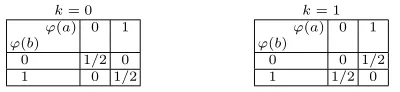
Ifk= 0,ϕ(a) =ϕ(g(a, k)). Ifk= 1,ϕ(a) = 1−ϕ(g(a, k)) mod 2.
The distributions S(g,0) andS(g,1) are drawn in Table 1. These two distribu-tions are definitely different. So given any distribution, we are able to determine what subkeykwas used to produce it.
k= 0 k= 1
ϕ(a) 0 1
ϕ(b)
0 1/2 0
1 0 1/2
ϕ(a) 0 1
ϕ(b)
0 0 1/2
1 1/2 0
Table 1: Joint distribution of (a, b=a⊕k) inZ/2Z
We have computed the theoretical distributions for several functions that in-volve a part of the key, like theexclusive-or between bytes, the DES S-boxes [27] and the AES SubBytes function [8]. All present some differences, even if the non linear functions present more differences. As the distributions of a function do not depend on a device, they may be pre-computed.
If the distributions are easily distinguished, that means the functiongcould be a good choice for an attack. However, an attacker will face two problems.
3
First, he must be able to get a distribution that will be compared to the theoretical ones, knowing he has access only to some traces. We suppose that he can acquire many traces he wants and that the trace number is sufficient for a uniform distribution of the input g function. This assumption is not restrictive because the cryptographic functions generally try to achieve this property. For obtaining a relevant distribution, the attacker needs also to locate the instants corresponding to the handling of the variablesaandb. As the traces contain some information but also noise, he will only be able toestimate the frequency of the couple (ϕ(a) =i, ϕ(b) =j) denotedfi,j. We nameSd={fi,j|i∈ {0, . . . , n}, j∈
{0, . . . , m}}the estimated distribution of the device. A solution for getting it is proposed in the next section.
The secondproblem the attacker faces is the need for a method to compare two distributions:
– S(g, k), which is theoretical. It is issued from the preliminary study and depends on the functiong and a key guessk.
– Sd, which is estimated. It is computed from the traces and related to the
device.
Section 4 examines the existing distances and selects the most promising ones for comparingS(g, k) andSd.
For the rest of this article, we consider that the functionϕ(z) represents the Hamming weight ofz,i.e.the number of 1 in binary representation. The function gis composed of the AES operations: AddRoundKey followed by SubBytes,i.e. the data a represents a state byte before the AddRoundKey and the datab a state byte after the SubBytes. Notice that otherϕmodels and otherg functions could be studied.
3
How to Estimate the Distribution of the Device
We suggest here a method to first identify the suitable instants and then estimate the Hamming weight values that they represent. These instants, named points of interest, are denoted byPoI.
To determine the most interesting instants of our traces, we used the variance. The higher the variance, the more favorable the instant, because it represents either the maximal variability of the noise or the maximal variability of some data spend by the algorithm. Determining thePoI is an important part of our proposal. In some other cases, the attacker may need more advanced techniques like in [10,2,11], but this simple way is initially sufficient.
After selecting somePoI, we have to decide from their amplitude value what the corresponding Hamming weight value is.
We suggest here a method that does not recognize the exact Hamming weight value, but allows a reasonable estimation for a low time and memory complexity by using the only traces of the targeted device. The estimation we present is close to the value of the Hamming weight of the targeted data.
LetY(t) be a set of M measured values corresponding to the same instant t of M traces. We sort this set in an ascending order. As we suppose that the data values of the cryptographic algorithm are uniform, this implies a particular distribution of the Hamming weight values. Ifnis the maximal Hamming weight
value, among theM elements, M ×C
p n
2n elements have a Hamming weightp. The
elements ofY(t) are classified knowing this distribution. The maximal Hamming weight value is assigned to the highest elements of the setY(t) and the minimal Hamming weight value to the smallest one.
For example, if 100 values represent the leakage of two bits, we associate the Hamming weight of:
- 2 for the 100×C 2 2
22 = 25 greater elements
- 1 for the 100×C 1 2
22 = 50 following elements
- 0 to the 100×C 0 2
22 = 25 smaller elements
Indeed, the way to classify the elements depends on the leakage quality. This method is effective if the noise is low. So by reducing the noise, for example thanks to the cumulant of order 4 [15], the estimation will be better. Using this simple method, we obtain an approximation of the Hamming weight of the targeted variable. Further, one error in the ranking generally gives a Hamming weight close to the real one. Some total mistakes may occur and perturb the estimated distribution. In this case, more traces will be necessary for obtaining an estimated distribution close to the theoretical distribution corresponding to the true key. We also can choose to sort the M elements in fewer groups by reducingϕ. For example,ϕmay represent the most significant bit,i.e. ϕ(z) = 0 if the higher significant bit is zero, 1 otherwise. This implies fewer errors, but the function ϕis less precise and the theoretical distributions will be more similar. This technique has a low complexity in time and memory but only gives an estimation. This method can be easily replaced by method based on clustering and machine learning.
Since we have a way to approximate the Hamming weight of the input and the output of the AES SubBytes, we can compute an estimated distributionSd.
4
How to Compare Two Distributions
To confront the theoretical distribution S(g, k) and an estimated distribution Sd, the first idea is to use the well-knownχ2distance between them defined as:
χ2(S(g, k), Sd) = i=n
X
i=0
j=m
X
j=0
δ(pi,j, fi,j) (1)
The distance betweenpi,j andfi,j is defined by:
δ(pi,j, fi,j) =
(pi,j−fi,j)2
pi,j , pi,j6= 0 0 , pi,j=fi,j
∞ , pi,j= 06=fi,j
(2)
Unfortunately, this distance does not allow errors in the estimated distribu-tionSd. Indeed, a theoretical distribution generally presents a lot of zero values
pi,j, so a small mistake in the estimated Hamming weight can cause a non-zero
value for the correspondingfi,j. Thus the distance betweenSdandS(g, k⋆) will
be infinite with only one error.
So we need to find another distance. In [5], Cha proposes a comprehensive study of different distances between two distributions. We have tested all the 65 distances presented in this article by using the theoretical distributions based on the Hamming weight leakage and the AES SubBytes function.
When trying to match a distribution that is well estimated to the theoretical ones, most distances give similar results and return the good subkey with few samples. But if the device distribution is not well estimated because of the pres-ence of errors for some samples, some distances give better results than others. We simulated 50% erroneous samples4to obtain biased device distributions and tried all the distances to compare each estimated distribution to the theoritical ones. We kept the four following best distances, that are those that on average lead to a successful attack.
– The distance based on the Inner Product defined by:
dIP(S(g, k), Sd) = 1− i=n
X
i=0
j=m
X
j=0
pi,j.fi,j (3)
– The distance based on the Harmonic Mean defined by:
dHM(S(g, k), Sd) =
(
1−2.Pi=n
i=0
Pj=m
j=0
pi,j.fi,j
pi,j+fi,j , pi,j+fi,j 6= 0
0 , pi,j+fi,j = 0
(4)
4
– Theχ2Pearson distance
dχ2
P(S(g, k), Sd) =
Pi=n
i=0
Pj=m
j=0
(pi,j−fi,j)2
fi,j , fi,j6= 0
0 , fi,j=pi,j
∞ , fi,j= 06=pi,j
(5)
– The distance of Kullback-Leiber
dKL(S(g, k), Sd) =
(Pi=n i=0
Pj=m
j=0 pi,j.ln(pfi,ji,j) , fi,j6= 0
0 , fi,j= 0
(6)
With the study of the distributions of two variables related to the crypto-graphic algorithm, the method presented in Section 3 for estimating an equivalent distribution related to the device and the distances introduced here, we are now able to establish an attack in order to retrieve the subkeyk⋆.
5
The Proposed Attack
Our attack consists of four phases. First, we get the pre-computed theoretical distributions that are not device dependent. This part is described in Algo-rithm 1.
Algorithm 1 Computation of the theoretical distributions. 1: procedureComputation ofS(g, k)(g:K×A→B ,N=|K|) 2: fork∈Kdo
3: S(g, k)←0 ⊲ S(g, k)∈ {0. . . n} × {0. . . m} 4: fora∈Ado
5: S(g, k)(ϕ(a), ϕ(g(a, k)))←S(g, k)(ϕ(a), ϕ(g(a, k))) + 1
|A|
6: end for
7: end for
8: returnS(g, k) 9: end procedure
In the second step, we detect some PoI thanks to the variance criteria. We denote the found PoI by ta ∈ Ta for the input of our function g and by
tb ∈ Tb for the output. The third step consists of extracting the estimated
Hamming weights of eachY(ta) and eachY(tb) and computing several estimated
distributions Sd(ta, tb) for each ta ∈Ta and tb ∈Tb with the method described
in Section 3. Finally, we compute all the distances between the theoretical distributions and the different estimated distributions. The secret subkey for the couple ofPoI (ta, tb) will be given by:
k⋆= argmin k∈K
Algorithm 2 Our proposal Attack
1: procedureAttack(M estimated Hamming weight pairs (ai, bi))
2: g:K×A→B,N=|K| 3: fork∈Kdo
4: S(g, k)←0 ⊲ S(g, k)∈ {0. . . n} × {0. . . m}
5: fora∈Ado ⊲Compute the theoretical distributions
6: S(g, k)(ϕ(a), ϕ(g(a, k)))←S(g, k)(ϕ(a), ϕ(g(a, k))) + 1
|A|
7: end for
8: end for
9: Sd←0 ⊲ Sd∈ {0. . . n}x{0. . . m}
10: forifrom0toM−1do ⊲Compute the estimated distribution 11: Sd(ai, bi)←Sd(ai, bi) +M1
12: end for
13: key←0
14: fork∈Kdo ⊲Compare the estimated distribution to the theoretical distributions
15: if d(S(g, k), Sd)< d(S(g, key), Sd)then
16: key←k
17: end if
18: end for
19: returnkey
20: end procedure
We name the number of samplesM, the number of possible keys N =|K|. We describe our attack in Algorithm 2.
Our algorithm complexity is:
- First step: one multiplication andN · |A| additions for the computation of the theoretical distributions.
- Second step: one multiplication andM additions for the computation of the estimated distribution.
- Third step:N·n·mmultiplications and 1 +N·n·madditions to compute N distances based on the Inner Product.
We notice that the complexity of the attack is low. The first step is performed once and for all. The cost of the attack depends on the sample number for the second step and on the key number for the last step.
6
Experimentations
6.1 Unprotected software implementation on ATMega2561
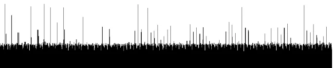
First, we need to ensure that our methodology for estimating the Hamming weight gives good results. We have acquired 1,000 samples on our device. The different AES steps can be distinguished on the traces (see Figure 1). We consider the nine instants with a variance greater than 10 times the average variance (see Figure 2 that is synchronized with Figure 1.).
As somePoI are poorly located regarding the region of the trace identified as the function AddRoundKey followed by SubBytes, we are able to identify some unusablePoI. For example, one of the PoI is localized at the beginning of the trace. FourPoI are situated in the SubBytes (SB) region and may there-fore correspond to the input of the targeted function. The four remainingPoI are positioned in the MixColumn (MC) region and may be associated with the output of the SubBytes function.
Figure 1: Electromagnetic emanation signal from an ATMega2561 during the execution of the first round of an AES128 software implementation.
Figure 2: Variance obtained for 1,000 electromagnetic emanation signals from an ATMega2561 during the execution of the first round of an AES128 software implementation.
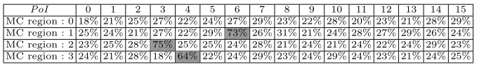
per-centage of good Hamming weight estimations for the fourPoI in the SubBytes region (resp. in the MixColumn region) for all the state bytes.
PoI 0 1 2 3 4 5 6 7 8 9 10 11 12 13 14 15
SB region : 0 24% 21% 28% 18% 78% 22% 24% 29% 23% 24% 29% 24% 23% 21% 24% 25% SB region : 1 21% 19% 20% 27% 24% 21% 25% 24% 26% 21% 29% 22% 24% 24% 28% 23% SB region : 2 25% 24% 21% 27% 22% 29% 81% 26% 31% 21% 24% 28% 27% 29% 26% 24% SB region : 3 22% 23% 24% 68% 21% 27% 23% 25% 23% 31% 25% 21% 23% 25% 21% 22%
Table 2: Percentage of good Hamming weight estimations for the input of the targeted function for all the state bytes.
PoI 0 1 2 3 4 5 6 7 8 9 10 11 12 13 14 15
MC region : 0 18% 21% 25% 27% 22% 24% 27% 29% 23% 22% 28% 20% 23% 21% 28% 29% MC region : 1 25% 24% 21% 27% 22% 29% 73% 26% 31% 21% 24% 28% 27% 29% 26% 24% MC region : 2 23% 25% 28% 75% 25% 25% 24% 28% 21% 24% 21% 24% 22% 24% 29% 23% MC region : 3 24% 21% 28% 18% 64% 22% 24% 29% 23% 24% 29% 24% 23% 21% 24% 25%
Table 3: Percentage of good Hamming weight estimations for the output of the targeted function for all the state bytes.
As the implementation handles byte by byte, one PoI corresponds to, at most, one state byte. So the estimator shall associate many correct Hamming weight values to, at most, one state byte. For the other state bytes, the number of correct Hamming weight values is close to a random estimation. For example, we can remark that the firstPoI in SubBytes region shall represent the state byte 4 before AddroundKey. Thus the estimator gives us a good approximation of six bytes, each one corresponding to onePoI.
We conclude that our estimator gives good results, at least for the trace instants where the variance is high. Thus an attacker could directly use the variance criteria and the identification of the trace blocks to choose thePoI. Of course, he does not have the means to verify the estimation method because he does not know the key value.
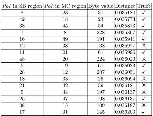
Finally, we have to validate the proposed attack. Luckily, the chosenPoI give Hamming weight values that correspond to the same state byte before and after the targeted function. So we expect to find the bytes 3, 4 and 6 of the subkey. Four PoI have been considered by region, so 4×4 = 16 pairs (ta, tb)
PoI in SB regionPoI in MC region Byte value Distance True?
2 1 54 0.0036051 X
3 2 31 0.0036711 X
0 3 61 0.0037023 X
3 3 224 0.0037423 X
0 0 200 0.0037556 X
2 3 234 0.0037823 X
2 0 39 0.0037883 X
1 3 154 0.0037976 X
3 0 55 0.0037986 X
0 2 216 0.0038011 X
1 1 159 0.0038514 X
2 2 206 0.0038786 X
1 2 21 0.0038983 X
3 1 218 0.0039113 X
0 1 257 0.0039115 X
1 0 197 0.0039612 X
Table 4: Attack results for the 4×4 chosenPoI.
PoI in SB regionPoI in MC region Byte value Distance True?
8 23 31 0.035180 X
42 18 23 0.035773 X
33 45 54 0.035813 X
1 8 228 0.035867 X
16 49 191 0.035941 X
12 38 138 0.035977 X
11 21 61 0.035996 X
48 20 224 0.036023 X
5 19 61 0.036023 X
28 12 207 0.036051 X
13 33 25 0.036094 X
21 42 39 0.036121 X
9 34 197 0.036137 X
25 47 198 0.036137 X
38 15 109 0.036187 X
17 31 145 0.036203 X
Table 5: The top 16 attack results for the 50 PoI with the higher variance for each region.
We have also performed the attack by using the other distances of Cha’s article [5]. This leads to worse results and validates the choice of the Inner Product distance.
The targeted implementation is eight bits, but it is also possible to attack a 16-bit implementation. This implies computing more distributions that are larger, but their computation can be performed in less than a half hour.
More, if the implementation provides a data masking countermeasure, our proposal can still be effective by targeting the AddRoundKey operation instead of the SubBytes.
6.2 DPAContest V4 [28]
In the 2013 summer, the DPA contest version 4 [28] has been released. It provides 100,000 samples corresponding to the first round and the beginning of the second round of an AES-256 software. So we focus only the first subkey.
The SubBytes function in the AES is replaced by sixteen masked sboxes:
SB(X⊕Mi+j mod 16⊕K)⊕Mi+1+jmod 16
where M0. . . M15 are the bytes of the mask andi is the sbox number. As the value of the 16-byte mask is known, this function contains two unknowns values: the secret byte subkeyK and also the valuei+j.
We decide to retrieve these two values together by using our method. If the offsetj is fixed, the knowledge of i+j is an advantage as it gives the relative position between the finding bytes. This hugely reduces the number of remaining keys in the exhaustive search.
As previously we have selected 1,000 PoI by using the variance. But this time we use four distances:
– Inner Product – Harmonic mean – Pearsonχ2 – Kullback-Leiber
These four distances will give different results, but we expect that the good key byte will has a good rank for each distance. The idea is to compute the top 16 attack results for each distance and each pair ofPoI. Then we keep only the results for each pair that appear for all distances. Finally the first 16 most frequent values are proposed for the subkey. We found 7 ordered bytes of the secret subkey. It is important to notice that here we only have 7·29·8 ≈ 275 remaining subkeys.
We have applied the same attack on another class of traces by considering the other offset values and compared the different results. The same bytes of the subkey have been obtained. More secret key bytes could be retrieved with the acquisition of the AES next rounds.
7
Conclusion
Indeed, we have validated both the estimation method and the key recovery by applying our attack on two sets of acquisition. The first one contains 1,000 traces issued from an AES128 software implementation into an ATMega2561. The results show that 10 disordered key bytes can be retrieved without any knowledge of the plaintext or the ciphertext. The second one comes from the DPA contest v4. Here we found 7 ordered bytes of the key.
The software context is well adapted to estimate the joint distribution of two internal data sets because few bits are processed at the same time. Attacking a hardware implementation in this manner remains a challenge, as it involves a huge bit number. This represents an easy way to protect a cryptographic algorithm. However, our attack may be also relevant for non-cryptographic op-erations like masking or reverse engineering.
References
1. M.L. Akkar, C. Giraud.An Implementation of DES and AES secure against some attacks. CHES 2001, LNCS vol. 2162 pp. 309–318, 2001.
2. C. Archambeau, E. Peeters, F.-X. Standaert, J.-J. Quisquater.Template Attacks in Principal Subspaces. CHES 2006, LNCS, vol. 4249, pp. 1-14, 2006.
3. A. Bogdanov.Improved Side-Channel Collision Attacks on AES. SAC 2007, LNCS, vol. 4876, pp. 84-95, 2007.
4. E. Brier, C. Clavier, F.Olivier. Correlation power analysis with a leakage model. CHES 2004, LNCS, vol. 3156, pp. 16-29, 2004.
5. S.-H. Cha. (2007)Comprehensive survey on distance/similarity measures between probability density functions. International Journal of Mathematical Models and Methods in Applied Science, 1 (4), 300–307, 2007.
6. S. Chari, J. Rao, P.Rohatgi.Template Attack. CHES 2002, LNCS, vol. 2523, pp. 13-28, 2002.
7. C. Clavier, B. Feix, G. Gagnerot, M. Roussellet, V. Verneuil.Improved Collision-Correlation Power Analysis on First Order Protected AES CHES 2011, LNCS, vol 6917, pp 49-62, 2011.
8. J. Daemen, V. Rijmen.AES proposal: Rijndael, 1998.
9. B. Debraize.Efficient and Provably Secure Methods for Switching from Arithmetic to Boolean Masking. CHES’12, LNCS, vol. 7428, pp. 107–121, 2012.
10. B. Gierlichs, L. Batina, P. Tuyls, B. Preneel. Mutual Information Analysis - A Generic Side-Channel Distinguisher. CHES 2008, LNCS, vol. 5154, pp. 426-442, 2008.
11. B. Gierlichs, K. Lemke-Rust, C. Paar. Templates vs. stochastic methods. CHES 2006, LNCS, vol. 4249, pp. 15-29, 2006.
12. L. Goubin, J. Patarin. DES and Differential Power Analysis - The duplication method. CHES ’99 LNCS vol. 1717, pp. 158-172, 1999.
13. M. Joye, P. Paillier, B. Schoenmakers.On Second-Order Differential Power Anal-ysis.CHES 2005, LNCS vol. 3659, pp. 293–308, 2005.
14. P.C. Kocher, J. Jaffe, B. Jun.Differential power analysis. CRYPTO, pp. 388-397, 1999.
16. S. Mangard, E. Oswald, T. Popp.Power Analysis Attack - Revealing the Secret of Smart Cards. Springer, 2007.
17. T. Messerges. Using Second-order Power Analysis to Attack DPA Resistant Soft-ware. CHES 2000 LNCS vol. 1965, pp. 238-251, 2000.
18. E. Oswald, S. Mangard, C. Herbst, S. Tillich.Practical Second-Order DPA Attacks for Masked Smart Card Implementations of Block Ciphers. CT-RSA 2006 LNCS vol. 3860, pp. 192–207, 2006.
19. E. Oswald, S. Mangard, N. Pramstaller. Secure and Efficient Masking of AES - A Mission Impossible? Cryptology ePrint Archive, Report 2004/134, http://eprint.iacr.org/2004/134.
20. M. Rivain.On the Physical Security of Cryptographic Implementations. PhD thesis, University of Luxembourg, 2009.
21. M. Nassar, Y. Souissi, S. Guilley, J.-L. Danger.RSM: A small and fast counter-measure for AES, secure against 1st and 2nd-order zero-offset SCAs. DATE 2012, pp 1173-1178, 2012.
22. M. Rivain, E. Prouff, J. Doget. Higher-Order Masking and Shuffling for Software Implementations of Block Ciphers. CHES 2009, LNCS, vol. 5747, pp. 171–188, 2009.
23. M. Renauld , F-X.Standaert.Algebraic Side-Channel Attacks. Cryptology ePrint Archive, report 2009/279, http://eprint.iacr.org/2009/279.
24. M. Renauld, F.-X. Standaert, N. Veyrat-Charvillon. Algebraic Side-Channel At-tacks on the AES: Why Time also Matters in Differential Power Analysis. CHES 2009, LNCS, vol. 5746, pp. 97-111, 2009.
25. M. Saied Emam Mohamed, S. Bulygin, M. Zohner, A. Heuser, M. Walter Im-proved Algebraic Side-Channel Attack on AES Cryptology ePrint Archive, report 2012/084, http://eprint.iacr.org/2012/084.
26. K. Schramm, T.J. Wollinger, C. Paar. A new class of collision attacks and its application to Des. FSE’03, LNCS, vol. 2887, pp. 206-222, 2003.
27. Federal Information Processing.Data Encryption Standard. Standards Publication 46-1 National Technical Information Service, U.S. Dept. of Commerce, 1977. 28. DPA contest v4.http://www.dpacontest.org/v4/