A Neural Model of Contour Integration in the Primary
Visual Cortex
Zhaoping Li
Hong Kong University of Science and Technology, Clear Water Bay, Hong Kong
Experimental observations suggest that contour integration may take place in V1. However, there has yet to be a model of contour integration that uses only known V1 elements, operations, and connection patterns. This article introduces such a model, using orientation selective cells, local cortical cir-cuits, and horizontal intracortical connections. The model is composed of recurrently connected excitatory neurons and inhibitory interneurons, re-ceiving visual input via oriented receptive fields resembling those found in primary visual cortex. Intracortical interactions modify initial activity patterns from input, selectively amplifying the activities of edges that form smooth contours in the image. The neural activities produced by such interactions are oscillatory and edge segments within a contour os-cillate in synchrony. It is shown analytically and empirically that the extent of contour enhancement and neural synchrony increases with the smoothness, length, and closure of contours, as observed in experiments on some of these phenomena. In addition, the model incorporates a feed-back mechanism that allows higher visual centers selectively to enhance or suppress sensitivities to given contours, effectively segmenting one from another. The model makes the testable prediction that the horizon-tal cortical connections are more likely to target excitatory (or inhibitory) cells when the two linked cells have their preferred orientation aligned with (or orthogonal to) their relative receptive field center displacements.
1 Introduction
In early stages of the visual system, individual neurons are responsive only to stimuli in their classical receptive fields (RFs), which are only large enough to signal a small edge or contrast segment in the input (Hubel & Wiesel, 1962). The visual system must group separate local input elements into meaningful global features to infer the visual objects in the scene. Some-times local features group together into regions, as in texture segmentation; at other times, they group into contours that may represent boundaries of underlying objects. Although much is known about the early visual pro-cessing steps that extract local features such as oriented edges, it is still unclear how the brain groups local features into global and more meaning-ful features. In this study, we model the neural mechanisms underlying the
first stages of grouping of edge elements into contours—namely, contour integration.
One of the first problems for contour grouping is the abundance of can-didate “edges” produced by the simple edge detection mechanism that is believed to operate in V1 (Marr, 1982). Many of these edges are simply im-age contrast noise and are unlikely to belong to any significant or relevant object contour. It is desirable to influence the response of edge detectors by contextual information from the surround to enhance the sensitivity to more relevant edges. This could be the first step toward perceptual con-tour grouping. Indeed, V1 cells are observed to change their responses or sensitivities depending on the surround stimulus (Knierim & van Essen, 1992; Kapadia, Ito, Gilbert, & Westheimer, 1995); cells are more responsive if they are stimulated by edges that are aligned with other edge elements outside their RFs (Kapadia et al., 1995). These observations correspond well with psychophysical observations that human sensitivity to edge segments is also higher when they are aligned with other edges (Polat & Sagi, 1994; Kapadia et al., 1995). Horizontal cortical connections linking cells of non-overlapping RFs have been observed and hypothesized as the underlying neural substrate (Rockland & Lund, 1983; Gilbert, 1992). These findings sug-gest that simple and local neural interactions even in V1 could contribute to primitive visual perceptual grouping as in contour integration, although V1 cells have been observed to change their sensitivities by visual attention (Motter, 1993).
hardware. Many computer vision models of edge linking (e.g., Kass, Witkin, & Terzopoulos, 1988) need user intervention, and many more autonomous models (e.g., Shashua & Ullman, 1988; Guy & Medioni, 1993; Williams & Jacobs, 1996) suffer from one or another problem. It is thus desirable to find out whether contour enhancement can actually be modeled using just V1 neural elements and operations, or whether contour enhancement in V1 has to be totally attributed to top-down feedback.
This article introduces a model of contour enhancement using only V1 el-ements, based on experimental findings, such as orientation selective cells, local recurrent neural circuits, and finite-range horizontal connections. The model is studied analytically and empirically to understand how sensi-tivity enhancement in long-range contours is successfully carried out in a network of neurons with finite-range interactions. The network dynam-ics are analyzed to reveal the temporal synchrony between cells within a contour, as observed in experiments (Gray & Singer, 1989; Eckhorn et al., 1988). Our analysis relates the extent of the contour enhancement and neu-ral synchrony with contour characteristics such as length, curvature, and closure. The model makes a testable prediction about the horizontal connec-tion structure: the postsynaptic cell type is more likely to be excitatory (or inhibitory) if two cells linked by the horizontal connection prefer orienta-tions that are aligned (or orthogonal) to the relative displacement between their RF centers. In addition, this model introduces a mechanism that allows higher visual centers selectively to enhance or suppress contour sensitivi-ties, in addition to the contour enhancement performed within V1.
Our work is mainly aimed at modeling the aspects of contour enhance-ment that are observed in V1. Contour integration is most likely completed by higher visual centers, which are absent in our model. This is in contrast to many other models that aim to build a model with the best possible per-formance at contour integration rather than to understand how and where it is done in the brain. For instance, this model does not address or define illusory contours, since V1 cells are not as evidently responsive to illusory contours as are V2 cells (von der Heydt, Peterhans, & Baumgartner, 1984; Grosof, Shapley, & Hawken, 1993), and T, L, X junction units, which are not known to exist in V1, are required to detect many types of illusory contours. (However, our model does help to fill in the gaps in incomplete contours; see section 3.) Also, assuming that V1 does not address contours as global objects, the model merely enhances individual contour segments, without defining the saliency of a whole contour. Additionally, a mechanism of feed-back control is provided by modeling the feedfeed-back signals and specifying their V1 target neurons, but we do not actually model how higher visual centers might respond to V1 outputs in order to construct the desired feed-back.
enhancement and synchronization depend on contour characteristics. The performance of the model is demonstrated by examples. Then we model the top-down feedback and demonstrate selective enhancement, suppression, and the effective segmentation by top-down control. Finally, we place the model in the context of experimental findings and other models, and discuss its limitations and possible extensions.
2 Experimental Background
Primary cortical neurons respond to input edges only within their classical receptive fields, which are local regions in the visual field mostly too small to contain any visual object (Hubel & Wiesel, 1962). RF centers are dis-tributed visuotopically on the cortical surface and cells with overlapping RFs, but different preferred edge orientations are grouped together into hy-percolumns (Hubel & Wiesel, 1962). Visual stimuli outside a cell’s classical RF, in a region whose size is larger than the RF, can influence the responses of the cell (see Allman, Miezin, & McGuinness, 1985; Knierim & van Essen, 1992). Generally, antagonistic suppression is observed when gratings or tex-tures are presented in the surround (Allman et al., 1985), although surround facilitation (Maffei & Fiorentini, 1976) and orientation contrast facilitation have also been observed (Sillito, Grieve, Jones, Cudeiro, & Davis, 1995). By placing bars in the surround of the RF of a cell and roughly aligning them with a bar presented in the center in its preferred orientation, Kapadia et al. (1995) demonstrated a significant increase in response to the central bar, even when there are additional random stimuli in the background. This enhancement of response decreases with increasing separation or misalign-ment between the central and surround bars, and is stronger when multiple bars in the surround are aligned with the central bar to generate a smooth contour (Kapadia et al., 1995). Such contextual influences will be the mecha-nism used for the contour enhancement in our model. Qualitatively similar findings are observed psychophysically in humans under similar stimulus settings (Polat & Sagi, 1994; Kapadia et al., 1995). Human observers can also easily identify a smooth contour composed of individual or even discon-nected edge segments among other random edge segments scattered in the background (Field, Hayes, & Hess, 1993). The sensitivity to such contours is enhanced when the contour closes on itself; this is called the closure effect (Kovacs & Julesz, 1993). Also, responses of V1 cells are modulated by visual attention (Motter, 1993), although earlier studies found these effects only in higher visual areas (Moran & Desimone, 1985).
layers and different groups of excitatory cells (and inhibitory cells), and they are likely to serve different functions; some cells are more concerned with receiving visual inputs, whereas other cells process the signals and send outputs to higher visual centers (Salin & Bullier, 1995). It is not yet clear what the target cell types are for the higher center feedback (Salin & Bullier, 1995). Cortical neurons interact with each other locally and often reciprocally; the excitatory connections extend somewhat longer distances than the inhibitory ones (Douglas & Martin, 1990; White, 1989). These neural interactions typically link neurons with similar RF properties (White, 1989). The anatomical basis for the surround effect has been postulated to be the long-range horizontal connections linking cells up to 4 mm or more apart in the primary visual cortex (e.g., Kapadia et al., 1995; Gilbert, 1992; All-man et al., 1985). These connections eAll-manate from the excitatory pyramidal cells in upper layers and contact both the excitatory and inhibitory post-synaptic cells, enabling monopost-synaptic excitation and dipost-synaptic inhibition from one cortical site to another (Gilbert, 1992; McGuire, Gilbert, Rivlin, & Wiesel, 1991; Hirsch & Gilbert, 1991; Weliky, Kandler, Fitzpatrick, & Katz, 1995). The axonal fields of these connections are asymmetrical, extending for greater distances along one cortical axis than another (Rockland & Lund, 1983; Gilbert & Wiesel, 1983; Fitzpatrick, 1996). Cells preferring similar ori-entations tend to be linked (Ts’o, Gilbert, & Wiesel, 1986; Gilbert & Wiesel, 1989; Malach, Amir, Harel, & Grinvald, 1993) whether or not the relative dis-placements of their receptive field centers are aligned with or orthogonal to their preferred orientations (Gilbert & Wiesel, 1983).
The horizontal cortical connections are also implicated in the temporal synchrony of the 40–60 Hz oscillations of neural responses (Gray & Singer, 1989; Eckhorn et al., 1988). Take two neurons with nonoverlapping RFs and aligned optimal orientations. The synchrony of their firing is negligible if two bars sweep over the two RFs independently, is significant when the bars sweep together, and is the strongest when a long, single, sweeping bar extends over both RFs (Singer & Gray, 1995). Usually the degree of neural synchrony decreases with increasing separation between neurons (Singer & Gray, 1995; Eckhorn, 1994). The extent of the oscillatory neural activities is not completely certain (Singer & Gray, 1995). It will be shown in our model that for inputs that contain contours, the strength of the neural oscillation depends on contour characteristics such as length and smoothness. Both the synchrony and the enhancement of responses for aligned edges have been postulated as mechanisms underlying feature linking (Gilbert, 1992; Singer & Gray, 1995; Eckhorn, 1994).
3 The Contour Integration Model
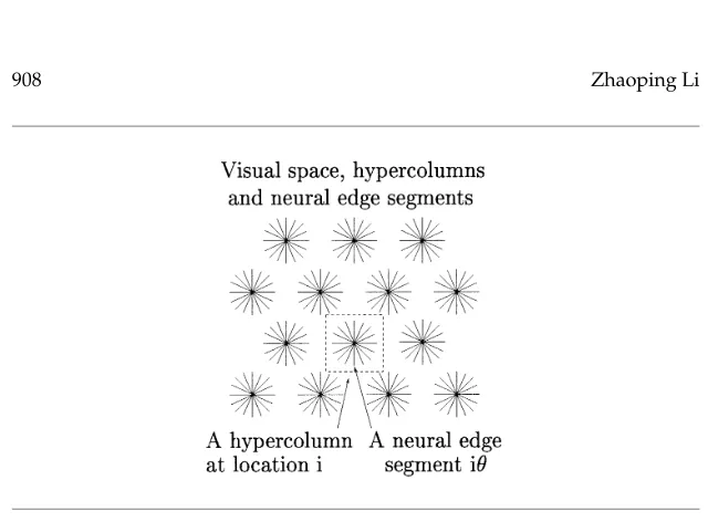
ana-Figure 1: Model visual space, hypercolumns, and edge segments. The input space is a discrete hexagonal or Manhattan grid.
lyzed and demonstrated. Next, the dynamics of the model are studied to reveal a tendency toward oscillations and the emergence of temporal coher-ence between contour elements. Finally, we introduce and demonstrate the mechanism that allows top-down feedback control.
3.1 Model Outline. Visual inputs are modeled as arriving at discrete spatial locations (see Figure 1). At each locationithere is a model V1 hy-percolumn composed ofKneuron pairs. Each pair(i, θ)has RF centeriand preferred orientationθ =kπ/K fork =1,2, . . . ,K, and is called (a neural representation of) an edge segment. Each edge segment consists of an ex-citatory and an inhibitory neuron that are connected with each other. The excitatory cell receives the visual input; its output quantifies the response or salience of the edge segment and projects to higher visual areas. The in-hibitory cells are treated as interneurons. When an input image contains an edge atiwith orientationβand input strengthIˆiβ, edge segmentiθreceives inputIiθ = ˆIiβφ(θ −β), whereφ(θ −β) = e−|θ−β|/(π/8) is the orientation tuning curve for the cell centered atθ. Segments outside the hypercolumn
ireceive no input contribution fromIˆiβ.
to visual inputs. Edge segmentjθ0 at another location can excite edgeiθ
monosynaptically by sending the excitatory signalJiθ,jθ0gx(xjθ0)to the exci-tatory cell in edgeiθ, and/or inhibit the edge disynaptically by directing an excitatory signalWiθ,jθ0gx(xjθ0)to the inhibitory cell. HereJiθ,jθ0andWiθ,jθ0
model the synaptic strengths of horizontal cortical connections. For any visual input patternIiθfor alli, θ, the neural dynamics evolve according to:
˙
xiθ = −αxxiθ−
X
1θ
ψ(1θ)gy(yi,θ+1θ)+Jogx(xiθ)
+X
j6=i,θ0
Jiθ,jθ0gx(xjθ0)+Iiθ+Io (3.1)
˙
yiθ = −αyyiθ+gx(xiθ)+
X
j6=i,θ0
Wiθ,jθ0gx(xjθ0)+Ic, (3.2)
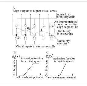
where 1/αxand 1/αyare the membrane time constants andIc is the back-ground input to the inhibitory cells, which will later be used to model top-down control signal.Iois the background input to the excitatory cells and includes a term that normalizes the activity—an inhibition that increases with the total activities in the local edge segments. Finally,ψ(1θ)is an even function of1θ modeling inhibition within a hypercolumn and decreases with|1θ|. Whenψ(1θ)=0 for1θ6=0, the inhibitory cells couple only to the excitatory cell in the same edge segment; otherwise, an activated edge exerts some inhibition∝ ψ(1θ)to other edges in the same hypercolumn. (Note that this interaction within a hypercolumn does not model the emer-gence of the cell orientation selectivity; Somers, Nelson, & Sur, 1995.) Each neuron additionally receives some random noise input. The appendix lists the parameters used in this model. For ease of analysis, and without loss of generality, we useαx =αy = 1, and makegx( )andgy( )piecewise linear functions with threshold and saturation. Also, the excitatory cells have a unit gaing0x(x)in the operating range.
Given an input patternIiθ, the network approaches a dynamic state after several membrane time constants, and the responsegx(xiθ)gives a saliency map. Whengx(xiθ)at locationiis a unimodal function ofθ (identifyingθ withθ +π), the orientationθ¯i that would be perceived in higher centers can be modeled byei2θ¯i ∝P
θgx(xiθ)ei2θ/Pθgx(xiθ). Two edges of different orientations will be perceived to cross each other at locationiifgx(xiθ)is a bimodal function ofθ.
3.2 A Single Edge Element. Before studying the contextual interactions between edges, we first analyze the input response properties of a single edge segmentiθ, ignoring the other edges. For simplicity, we omit the sub-scriptsiandθ, and denoteI=Iiθ+Io:
˙
x= −x−gy(y)+Jogx(x)+I. (3.3)
˙
Figure 2: (A) Model neural elements, edge elements, visual inputs, and neural connections.Jo: self-excitatory connection;J: lateral excitatory connection
be-tween edge elements;W: lateral disynaptic inhibitory connection between edge elements, implemented as excitatory connections from the excitatory neuron of one edge element to the inhibitory neurons of the others. (B) Activation function gx(x)for the excitatory cells. (C)gy(y)for the inhibitory cells.
The average neural activity is determined by the equilibrium point E = (x¯,y¯), which is the intersection of the two curves on whichx˙=0 andy˙=0, respectively (see Figure 3B):
˙¯
x=0= −¯x−gy(y¯)+Jogx(x¯)+I. (3.5)
˙¯
y=0= −¯y+gx(x¯)+Ic. (3.6)
IncreasingIorIcraises or lowers the outputgx(x¯). The input sensitivities, determined by solving the linearized version of the above equations, are
δgx(x¯)/δI=
g0x(x¯)
1+g0y(y¯)g0x(x¯)−Jog0x(x¯)
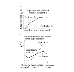
Figure 3: (A) Edge responsegx(x¯)as a function of visual input. Three response
curves—one solid and two dashed ones—are plotted for three different cortical inputsIcto the inhibitory cell. (B) Equilibrium point and curves for an edge
element. The solid curve is thex˙ =0 curve, and the dashed curve is they˙ =0 curve. IncreasingI raises thex˙ = 0 curve, and increasingIcraises, and
some-what deforms, the (monotonously increasing)y˙ = 0 curve, thus changing the equilibrium point(x¯,y¯). The neurons may approach the equilibrium point after some transient, or oscillate around it, as discussed in section 3.6.
δgx(x¯)/δIc =
−g0
y(y¯)g0x(x¯) 1+g0y(y¯)g0x(x¯)−Jog0x(x¯)
= −g0y(y¯)·[δgx(x¯)/δI]. (3.8)
In cases that interest us, the output gx(x¯) increases continuously with visual input I (see Figure 3A), that is, δgx(x¯)/δI ≥ 0, and this requires
threshold whereg0x=0 becomes nonzero after threshold whereg0x=1, and can decrease beyond threshold when the inhibitory gain g0y(y¯) increases. At highI, the activity gx(x¯) saturates when g0x = 0 again. Qualitatively, this sensitivity curve corresponds to physiological observations.1Note that threshold input valueI and the edge input response curve in Figure 3A change withIc. This is because, as shown in equation 3.8, increasingIc de-creases the outputgx(x¯).
According to equations 3.7 and 3.8, increasingIandIc simultaneously increases the outputgx(x¯)if1I/1Ic>g0y(y), and decreases it otherwise. This leads to the following consequences. First, the visual input could be directed to both the excitatory (increasingI) and inhibitory (increasingIc) cells as ex-perimentally observed (White, 1989). Their net effect will be to increase the edge responsegx(x¯)as long as the visual input partition to the two cell types is appropriate. Second, the effect of input from other edges via horizontal connections can be seen as increasingIand/orIc. Therefore, in general, the net contextual influence on the edge can be facilitatory or suppressive, de-pending on relative recruitment of horizontal fibers, as experimentally ob-served (Hirsch & Gilbert, 1991). Furthermore, since the gaing0y(y)increases with input level, such contextual influence is more likely to be inhibitory at higher input levels. This is also experimentally observed (Hirsch & Gilbert, 1991; Sengpiel, Baddeley, Freeman, Harrad, & Blakemore, 1995; Weliky et al., 1995). In our model, for simplicity, the visual input is directed solely to the excitatory cells, but this could easily be generalized. The horizon-tal connections in the model are specified (in section 3.3) such that the net contextual influence from appropriately aligned edges is facilitatory at all contrast levels, although the contextual influence from less aligned edges (these edges can still prefer similar orientations) can depend on stimulus levels. Hence, in this model, the change in the dominance between facilita-tory and suppressive contextual influences occurs only for input patterns that are not contours, and therefore is not going to be discussed further in this article.
3.3 Interactions Between Edge Segments for Contour Integration. Edge element(jθ0)excites or inhibits the edge element(iθ)by sending an excitatory-to-excitatory output Jiθ,jθ0gx(xjθ0) or an excitatory-to-inhibitory output Wiθ,jθ0gx(xjθ0). The goal for the connection structureJiθ,jθ0andWiθ,jθ0 is that edge elements within a smooth contour should enhance each other’s
activ-1When the segment has too strong a self-excitation—largeJ
og0x(x¯)—and not enough
inhibition—smallg0y(y¯), such thatg0y(y¯)g0x(x¯) <Jog0x(x¯)−1—the system is unstable, and
the outputgx(x¯)jumps discontinuously with inputI. Such cases are not considered here,
ities and that the isolated edge elements caused by noisy inputs should be suppressed, or at least not enhanced. Hence:
• The connectionJiθ,jθ0 will be large if one can find a smooth or small curvature contour to connect(iθ)and(jθ0), and it generally decreases with increasing curvature of the contour.
• Edge elements will inhibit each other viaWiθ,jθ0when they are
alter-native choices in the route of a smooth contour.
• Both connection types will decrease with increasing distances between the edge segments and become zero for large distances.
• The connections have translation, rotation, and reflection invariance. This means the following: Leti−jbe the line connecting the centers of two edges (iθ) and (jθ0), which form angles θ1 andθ2 with this connecting line. The connectionsJiθ,jθ0andWiθ,jθ0depend only on|i−j|,
θ1, andθ2, and satisfyJiθ,jθ0 =Jjθ0,iθandWiθ,jθ0=Wjθ0,iθ.
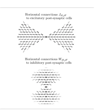
Given these requirements, connectionsJiθ,jθ0 andWiθ,jθ0 both link cells
that prefer similar orientations, as observed in experiments (Gilbert, 1992; Weliky et al., 1995) (see Figure 4). In addition, when the preferred orienta-tions of two linked cells are aligned with the relative displacement of their RF centers, the postsynaptic cell type is more likely excitatory (the connection
Jiθ,jθ0); when the preferred orientations are more or less orthogonal to the
rel-ative displacement of the RF centers, the postsynaptic cell type is more likely inhibitory (the connectionWiθ,jθ0). This provides a computational explana-tion to the puzzling experimental finding (Gilbert & Wiesel, 1983) that some horizontal connections link cells whose preferred orientations and relative RF center displacement do not align, but instead are roughly orthogonal to each other. These connections can serve to establish competition between alternative routes of a single contour by contacting inhibitory postsynaptic cells. This prediction (see the appendix for its derivation) of the model about the correlation between postsynaptic cell types and the degree of alignment between the two linked RFs has not been systematically investigated in experiments; a test is thus desirable. This excitatory and inhibitory edge interaction pattern is qualitatively similar to the edge compatibility func-tion in Zucker et al. (1989). Altogether, an edge in a smooth contour mostly receives facilitatory inputs Jiθ,jθ0gx(xjθ0) and few, if any, inhibitory inputs Wiθ,jθ0gx(xjθ0), from other edges in the contour. This helps to enhance the
of the edges in the contour significantly higher than the background noise. The strengths and weakness of the model are further demonstrated in Fig-ure 5B, where the model is challenged by the difficulties in a natural image.
3.4 A Straight Line. We can understand the performance of the model by analyzing some examples. In the first example, the visual input is a horizontal line on thex-axis
ˆ Iiθ=
½
Iline ifiis on the line andθ =0
0 otherwise. (3.9)
The inputsIcto the inhibitory cells of all edges are assumed to be the same. Let us consider the simplest case when edge elements outside the line (i.e., wheniis not on thex-axis orθ 6=0) are silent due to insufficient excitation. Then we can ignore all edges beyond the line, treat this system as one-dimensional, and omit indexθ. Letidenote the (one-dimensional) location of the line segment; thenWij=0, andJij≥0 for alli,j6=i, and
˙
xi= −xi−gy(yi)+Jogx(xi)+
X
j6=i
Jijgx(xj)+Iline+Io. (3.10)
˙
yi= −yi+gx(xi)+Ic. (3.11)
If the line is infinite, then by symmetry each neuron pair will have the same equilibrium point2E=(x¯,y¯)determined by:
˙¯
x=0= −¯x−gy(y¯)+Jogx(x¯)+(Iline+
X
j6=i
Jij
gx(x¯))+Io (3.12)
= −¯x−gy(y¯)+
Jo+
X
j6=i
Jij
gx(x¯)+Iline+Io (3.13)
˙¯
y=0= −¯y+gx(x¯)+Ic. (3.14)
This can be seen as either a single edge with extra external input1I= (Pj6=iJij)gx(x¯)or a giant single “edge” with a stronger self-excitatory con-nection(Jo+Pj6=iJij)(see Figure 6). Either way, activitygx(x¯)for each edge element in the line is enhanced (see Figures 5 and 7).
The same minimum strength of input is required to excite a segment in a line or an isolated edge (see Figure 6A), if all segments in the line are equally
2This equilibrium solution may or may not be stable, as studied in section 3.6.
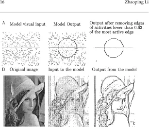
Figure 5: Contour enhancement and noise reduction. (A) Performance for a synthetic image. (B) Performance for an input obtained by edge detection from a natural photo. The input and output edge strengths are denoted proportionately by the thicknesses of the edges. The same format applies to other figures in this article. The model outputs are the temporal averages of gx(x)over a period
excited. This is because the line segments will have zero output before they reach threshold and so cannot excite each other. Therefore, they behave independently as isolated edges before threshold. However, when some line segments receive subthreshold and others have superthreshold visual inputs, the former can give nonzero output under contextual excitation from the latter. This leads to subthreshold activation or filling in for the weaker or missing segments in a line (or contour; see Figure 9C).
3.5 Curvature, Contour Length, and Contour Closure. Enhancement in contours other than lines can be understood based on the special case of a contour of a constant nonzero curvature, namely, a circle. It is apparent that the analysis for a straight line is also applicable here, assuming for simplicity that the corresponding circle for the contour has a diameter larger than the longest synaptic connection between cells. Indexiagain denotes the (one-dimensional) location of the segments along the (one-(one-dimensional) contour, and|i−j|the (one-dimensional) distance between the segmentsiandj. The activities of the elements along the contour are analogously enhanced.
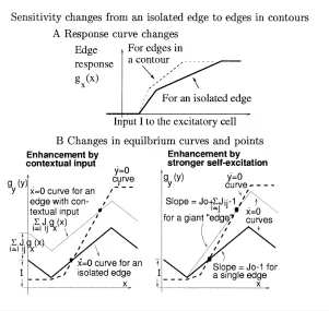
It can be shown from Figure 6B, after some geometrical calculation, that the response levels for a segment in a contour and an isolated segment differ by a factor(sy−s1)/(sy−s2)wheres1=Jo−1,s2=Jo+
P
i6=jJij−1, andsy is the slope of they˙=0 curve. The quantityPi6=jJijis the sum of horizontal connection strengths between one contour segment to all others; hence, it is larger for smoother contours by design, and thus the response enhance-ment is also larger for smooth contours.3 Furthermore, sinces
y is usually smaller for smaller input strength, the contour enhancement is stronger for low-input contrasts, which are the case in some physiological and psy-chophysical experiments (e.g., Kapadia et al., 1995; Kovacs & Julesz, 1993). Roughly, this model enhances the saliencies in a smooth contour against
Figure 5:Facing page, continued.
of a discrete sampling grid and a lack of a signal interpolation algorithm. In addition, two accidentally aligned but different contours (e.g., the contours for the hat, the hair line, and the cheek line near the right side of the image) can threaten to join each other because of the lack of T, L,and X junction signals that should prevent them. This model for contour enhancement also highlights region boundaries and pops out novelties (Li, 1997). Consequently, the edge segments for the hair pieces near the surrounds of the feather (even though the feather region is not very homogeneous), such as, the single feather across the brim, are more likely enhanced than those inside the feather. See the discussion in section 4.
3It can be shown that this conclusion still holds if some contour segments exert
Figure 6: Response changes from an isolated edge to edges in contours. All edges in a contour are assumed to receive the same visual input strength. (A) Changes in response curves. The solid curve is the response from an isolated edge, and the dashed curve is the response from edges in contours. (B) Changes in equilibrium curves and points. The two thick curves are thex˙ =0 (solid) and
˙
y= 0 (dashed) curves for an isolated edge. Only thex˙ = 0 curve is changed, going from an isolated edge (thick, solid curves) to edges in a contour (thin, solid curve). Such changes can be seen as caused by either extra excitationPj6=iJijgx(x)
from neighboring edge segments to a single edge (left figure) or an increase in the self-excitation or curve slopeJo−1→Jo+
P
j6=iJij−1 in a giant “edge.” The
equilibrium point changes from the lower black dot to the upper one.
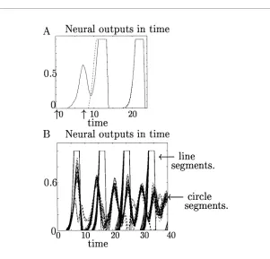
seen in Figure 7. These predictions are expected to hold also for contours of nonconstant curvature. Note that the line in Figure 7 is actually a closed line by the periodic boundary condition used in the model’s visual space. Since the line has zero curvature, its salience is higher than that of the circle. Note that edge segments in an open and a closed contour (see Figures 7b and 7c) have roughly the same saliency except near the ends of the open contour, where saliency decreases. This closure effect is weak compared to what is implied from psychophysical observation (Kovacs & Julesz, 1993; see section 4). Exactly how the saliency decays toward the ends depends on howJiθ,jθ0decays with intersegment distances and the longest connection
length. Note that the model used a discrete hexagonal grid in the visual space; the apparent small gaps in the circle and curves are the artifact of the coarseness of the grid.
3.6 Neural Oscillations and Synchrony Between Contour Segments. So far, we have analyzed only the equilibrium points(x¯,y¯), which are also roughly the average responses. Upon visual stimulation, the neurons may either approach the equilibrium after a transient phase or sustain dynamic activities about the equilibrium, such as oscillations. Here we show how variations of neural activities about their averages reflect characteristics of the contour.
Each edge segment, a pair of connected excitatory and inhibitory cells, can be modeled as a neural oscillator (Li & Hopfield, 1989) oscillating around the equilibrium point(x¯,y¯). With interactions between the segments, the os-cillators are coupled and exhibit collective behavior reflecting contour
acteristics embedded in the coupling. To analyze the dynamics, denote for simplicityxi− ¯xi→xi,yi− ¯yi→yi, and write as vectorsX=(x1,x2, . . . , )T
andY = (y1,y2, . . .)T. For smallXandY, we approximate by a linear
ex-pansion of equations 3.10 and 3.11 about the equilibrium point(x¯i,y¯i):
˙
X= −X−G0yY+JX (3.15)
˙
Y= −Y+G0xX, (3.16)
where4Jis a matrix with elements(J)ij=Jog0x(x¯j), ifi=j, and(J)ij=Jijg0x(x¯j) otherwise;G0xandG0yare diagonal matrices with elements(G0x)ii=g0x(x¯i) and(G0y)ii=g0y(y¯i). For a contour with a constant curvature (i.e., a circle), all its segments have the same equilibrium point if they receive the same input strength,x¯i = ¯xj ≡ ¯xandy¯i = ¯yj ≡ ¯y. ThenG0xandG0y are proportional to the identity matrix, andJis symmetric (since we imposed symmetry along contour directions, i.e., Jij = Jji). ThenJ has an orthogonal set of eigenvectors{Xk}and real eigenvaluesλkfork =1,2, . . .which we order such thatλ1≥λ2≥. . .Take{Xk}as the new basis to representXandY; we haveX=PkxkXk,Y=P
kykXk, and
˙
xk= −xk−g0y(y¯)yk+λkxk (3.17)
˙
yk= −yk+g0x(x¯)xk, (3.18)
which has solution
xk(t)=xk(0)e−(1−λk/2)tcos(ωkt+φk), (3.19)
where the oscillation frequency isωk = qg0
y(y¯)g0x(x¯)−(λk)2/4, and initial conditions determine the amplitudexk(0)and the phaseφk. The exponential in equation 3.19 suggests that the system will be dominated by the first os-cillation mode5X1sinceλ1≥λkfor allk. The relative oscillation amplitudes and phases of the segments in a contour are determined by the components of the complex vectorX1.
Let us suppose for simplicity that the edge segments concerned are in the linear operating region where g0x(x¯) = 1. For a contour of constant curvature with uniform inputs to its segments, matrix Jis Toplitz (i.e., Jij = J(i+a)modN,(j+a)modN for alla, whereN is the contour length or ma-trix dimension) under translation and rotation invariance of the model and
4Here we take for simplicity that contour segments do not link to each other with
connectionWiθ,jθ0. The analysis here needs a little modification, but the general conclusion still holds whenWconnections are included.
5From the analysis in the next paragraph, it will be apparent that it is unlikely to have
has nonnegative elements. It can then be shown that the eigenvectors are the cosine and sine waves along the contour, that is,Xkj ∝eifkjwith spatial
frequencyfkand the eigenvalues are the corresponding Fourier coefficients of the row vector of theJmatrix. In particular, the eigenvectorX1is the
zero-frequency Fourier wave; hence, all components ofX1are equal,x1i =x1j, and thus all segments in a contour oscillate with the same amplitude and phase. The eigenvalue for this mode is the zero-frequency Fourier coefficient, and thusλ1=J
o+Pallj6=ion contourJij. We can therefore relateλ1to the charac-teristics of the contour, as reflected by the connectionsJijalong its length. It follows that the strength of the oscillation is largest in a long line, decays with increasing contour curvature (or decreasing contour length for circles), and is weakest for an isolated edge. The isolated edge is a special case with a single oscillator (X1is a scalar) whenλ1=Jo. Whenλ1<2, the oscillation is dampened and disappears after some transient phase. Otherwise, if seg-ment couplings are sufficiently strong, the oscillations6will grow until the
nonlinearity invalidates the linear analysis and constrains the oscillation to have a finite amplitude (see the activities for the line segments in Figure 7). These predictions are expected to hold approximately for general contours with nonconstant curvatures or nonuniform inputs. However, because the translation invariance is compromised in these cases (i.e.,Jdeviates from be-ing Toplitz and symmetric), some differences in oscillation amplitudes and the relative phases are expected. Similarly, nonzero relative phases may emerge between edge segments near the end of a contour, or between such segments and those near the middle of the contour.
The role ofλ1 in the oscillation frequencyω1 =
q
g0y(y¯)g0x(x¯)−(λ1)2/4
suggests a correlation between stronger contours and lower oscillation fre-quencies, as is the case when comparing the circle with the line in Figure 7. However, in strong, sustained oscillations, the small-amplitude linear ap-proximation no longer holds. The nonlinearity greatly influences the fre-quency and makes this prediction imprecise. With strong visual input and contour enhancement, oscillation can be completely suppressed by the non-linearity near the saturation region. In realistic neural systems, however, sat-uration can be prevented by the gain control or adaptation for large inputs or activity levels.
Synchronization within a contour will happen even when the visual in-puts are turned on at different times for different contour segments. On the other hand, synchrony is rare between different contours even when their visual inputs are turned on simultaneously. These are both demonstrated
6For large enough λ1, the oscillation frequency from the linear analysis ω1 = p
g0y(y¯)g0x(x¯)−(λ1)2/4 is imaginary, so the local dynamics about the equilibrium point
in Figure 8; segments within a line quickly reach synchrony after asyn-chronous stimulus onset, but circle segments and line segments become out of synchrony within two oscillation cycles after synchronous stimulus onset. In fact, when two contours are nearby, they tend to desynchronize largely due to the normalizing neural interactions (see the appendix) and the mutual suppressive couplingsWiθ,jθ0between them. The dynamic
cou-pling between two contours also causes frequency shifts. Furthermore, the nature and synchrony of the oscillations of the weaker contour tend to be distorted by the stronger contour such that some of the contour segments oscillate in a nonsinusoidal manner (see Figure 8B). We do not discuss the details of such dynamic coupling further because they are not used for con-tour integration in this model. However, synchronization within a concon-tour and desynchronization between contours can be exploited for the purpose of contour segmentation (see section 4).
3.7 Control of the Contour Saliency by Top-Down Feedback: Selective Contour Enhancement/Suppression, Filling In, and Contour Segmenta-tion. This section shows that our model of V1 provides a mechanism by which higher visual areas can selectively influence the response to given contours. We just assume that the higher centers already know which seg-ments belong to a contour and what feedback signals to send back. In the model, the influence from higher centers is additional to, but not necessary for, the contour-enhancing capabilities by the V1 neural circuit.
Higher visual areas are modeled as sendingIcas a feedback signal to the inhibitory cells, to influence the edge outputs according to equation 3.8:
δgx(x¯)/δIc= −
g0y(y¯)g0x(x¯)
1+g0y(y¯)g0x(x¯)−Jog0x(x¯)
. (3.20)
LetIc=Ic,background+Ic,control. The background inputIc,backgroundis the same
for all edge segments, and can be used to modulate the overall level of visual alertness. Higher areas can selectively enhance or suppress a given contour by providing a negative or positiveIc,control(i.e., decreasing or increasing Ic) for the selected contour segments(iθ). A strong enoughIc,control>0 on
a given contour can completely suppress the outputs from that contour, leading to the effective removal or segmentation of this contour from other contours in the visual input.
It is not yet clear from experimental data which are the cells in V1 that should be the target of feedback (Salin & Bullier, 1995; also see section 4). This model chooses the inhibitory interneurons as the targets for the reason that it is computationally desirable not to mix visual inputs from the exter-nal world with the interexter-nal feedback sigexter-nals. Given that the excitatory cells are the visual input neurons in this model, directing the feedbacksIc,control
cannot completely substitute for visual stimulation. As is evident,Icis ef-fective only wheng0y(y¯)g0x(x¯)6=0. Without visual input or excitation from other segments, an edge segment’s membrane potentialx¯is below threshold andg0x(x¯) =0. Decreasing or removing the feedbackIc merely reduces or removes the inhibition onto this segment and is not enough to activate the excitatory cell beyond threshold when the background (nonvisual) input
Ioto the excitatory cell is too weak. However, with some, even subthresh-old, visual inputIiθ or contextual excitation from neighboring edges, an edge segment can increase its activity or become active ifIcis reduced or removed. Therefore, this model can enhance and complete or fill in a weak and incomplete input contour under the control of the feedback (see Fig-ure 9C), but cannot enhance or “hallucinate” any contour that does not at least partially exist in the visual inputI(see Figure 9B). See section 4 for more detailed discussion on the targets of the feedback, the related experimental findings, and computational considerations.
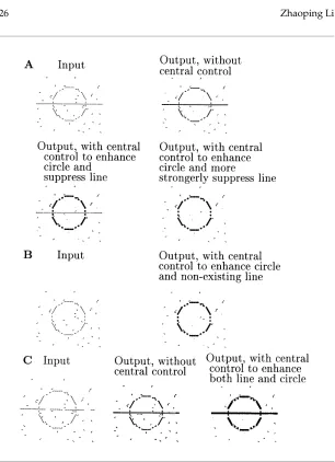
Figure 9 demonstrates central control. Without central control,Ic,control=
0, a visual input consisting of two contours, a circle and a line, and some noise segments results in a salient line and circle, and less salient noise segments (see Figure 9A). By addingIc,control>0 for the line andIc,control<0 for the
circle, the saliency of the line is suppressed, and the circle becomes most salient. If feedback controlIc,control> 0 for the line is strong enough, then
its neural activity can be completely eliminated, effectively segmenting it away from the circle (see Figure 9A). Without central control, the gaps in an input line are partially filled in by the excitation from other line segments (see Figure 9C); with reducedIc on the line, the initially fragmented line becomes almost completely filled in (see Figure 9C).
4 Summary and Discussion
orientation selective cells, a local neural circuit with recurrent interactions between excitatory and inhibitory cells, and the particular connection pat-terns suggested by experimental evidence (Gilbert, 1992; Hirsh & Gilbert, 1991; Weliky et al., 1995; White, 1989; Douglas & Martin, 1990; Kapadia et al., 1995). The neural interactions in the model enhance the cell activities for edge segments belonging to smooth contours against a background of ran-dom edge segments and induce synchronized oscillatory neural activities between segments within a contour. We show analytically and empirically that the extent of contour enhancement and neural synchrony is stronger for longer, smoother, and closed contours. These behaviors of the model are consistent with experimental observations (Kapadia et al., 1995; Field et al., 1993; Kovacs & Julesz, 1993; Gray & Singer, 1989; Eckhorn et al., 1988). In addition, this model introduces a mechanism that allows higher visual areas to feed back and selectively enhance or suppress activities for given contours, and even to achieve a crude form of contour segmenta-tion. This model makes the following testable predictions, which have not been systematically investigated experimentally: (1) the horizontal cortical connections from the excitatory cells should more likely contact excitatory or inhibitory postsynaptic cells if the two linked cells have their preferred orientations roughly parallel or orthogonal, respectively, to their relative RF displacement; (2) the strength of neural oscillation, as well as neural synchrony, should increase with contour length, smoothness, and closure.
For analytical tractability and simplicity, the model adopts the following idealizations: a 1:1 ratio between the excitatory and inhibitory cell numbers, the lack of connections between the inhibitory cells, and the lack of direct visual input to the interneurons. Without essential changes to the model per-formance, these idealizations can be relaxed to give additional complexities in model behavior. For instance, each model cell should be seen as mod-eling a local group of cells of similar types. Hence, the 1:1 ratio between the excitatory and inhibitory model cell numbers is really a ratio between local cell groups, and the recurrent local connections between them model the recurrent connections in the local cell groups. Also, introducing direct visual inputs to the inhibitory cells can give additional input gain control to allow a larger dynamic range for the system.
The recurrent local interactions between excitatory and inhibitory cells used in this model have long been part of a “basic circuit” for the cerebral cortical organization (Shepherd, 1990). They have been used, for instance, in a model of the olfactory bulb for odor recognition and segmentation (Li & Hopfield 1989; Li, 1990). A closely related version of this circuit is also used in a model of visual cortical RFs and surround influences (Somers, Todorov, Siapas, & Sur, 1995).
Our model requires a neural connection structure with both a colinear excitatory componentJiθ,jθ0and flanking or orthogonal and disynaptically
inhibitory componentWiθ,jθ0. A similar connection structure, where the
et al. (1989). A connection structure like our colinear excitatory connection componentJiθ,jθ0 is termed “association field” by Field et al. (1993) and is generic for many contour enhancement models (e.g., Zucker et al., 1989; Braun et al., 1994; Yen & Finkel, 1997). Experimentally, however, cortical cells have horizontal axonal fields that extend orthogonally as well as par-allel (colinearly) to the preferred orientation of the cells (Gilbert & Wiesel, 1983). The “association field” like connections can account for only those axons that extend in a roughly parallel direction. Our model suggests that the orthogonally extending axons (see Figure 4) should be found to con-tact preferentially inhibitory postsynaptic cells (the connectionWiθ,jθ0), for
the computational purpose of mediating competition between alternative routes of a contour. The different functions served by the different branch directions of the horizontal axons lead naturally to the anisotropic horizon-tal axonal fields as observed in V1 (Gilbert & Wiesel, 1983; Fitzpatrick, 1996). The quantitative degree of anisotropy in the axonal field is not crucial in this model. The predicted correlation between axon directions and postsynaptic cell types has yet to be experimentally tested.
4.2 Higher Center Feedback. The feedback control mechanism in the model may also relate to the attentional effects observed in V1 cells (Motters, 1993). It has the desirable property that while higher areas can enhance input contours, and even fill in the gaps in an incomplete contour, they cannot create a contour that does not exist in visual input. This property could be exploited by the higher visual centers to test hypotheses about the visual input and cooperate with V1 to reconstruct a coherent percept.7A complete
model of top-down, bottom-up cooperation should include a mechanism by which higher areas can respond to V1 outputs and construct the requisite top-down control signals. This mechanism is left for future work.
Experimental data have suggested both excitatory (Mignard & Malpeli, 1991; Nault, Michaud, Morin, Casanova, & Molotchnikoff, 1990) and in-hibitory (Alonso, Cudeiro, Rerez, Gonzalez, & Acuna, 1993; Fitzpatrick, personal communication, 1996) effects of feedback signals. Most data on feedback fibers show that feedback terminals synapse onto dendritic spines (Rockland, personal communication, 1996; Johnson & Burkhalter, 1992), which are usually associated with excitatory cells, though earlier obser-vations from Johnson and Burkhalter (1991) suggest that feedback fibers terminate near inhibitory interneurons. Although the evidence is not consis-tent or clear-cut (Salin & Bullier, 1995), some points in the opposite direction from our model construction that higher-center feedbacks are directed to the inhibitory interneurons. Computationally, I believe that it is important not
7In this model, the “hallucination” is prevented by setting the background inputI o
sufficiently low such that excitation byIoalone without visual input is impossible even
to mix bottom-up visual input signals with top-down feedback ones. Hence the feedback fibers should avoid the input neurons, which in this model are the excitatory cells. Indeed, in the brain, feedback fibers generally avoid cortical layer 4, which is the input layer (Salin & Bullier, 1995). Experimental evidence also suggests that top-down feedback to V1 can modulate V1 ac-tivities, but cannot substitute for visual input to activate V1 (Salin & Bullier, 1995). If hallucinations should be avoided in the visual system, then, as is shown in section 3, it helps to send the feedback via the inhibitory interneu-rons, as is done in this model. More realistically, V1 has different layers and groups of excitatory cells. Different excitatory cell groups are likely to serve different functions, and “hallucinations” may be avoided when the feedback fibers target other excitatory cells and avoid the excitatory cells in the input layer. It is also likely that top-down feedback first contacts the noninput excitatory cells, which then transform the signals to the inhibitory interneurons. Such signal transformations may be needed in order to render the visual representations in the higher areas in terms of the representation in V1. It is also likely that the feedback effects are dynamically modulated and can be excitatory or inhibitory, depending on the levels of neural ac-tivity and contextual conditions that are beyond the current model. More consistent and informative experimental data are desired to guide our fur-ther understanding. It is more clearly established in the lateral geniculate nucleus (Salin & Bullier, 1995) and the olfactory bulb (Shepherd, 1990) that higher-area feedback terminates mostly onto the inhibitory interneurons. It will be interesting to explore the extent of the universality of computational mechanisms across stages and sensory modalities. An analogous model of higher center control and olfactory segmentation has been proposed for the olfactory bulb (Li, 1990).
curva-ture, and closure for reasonably smooth contours are not very significant. This could be a weakness or strength of this model, depending on whether one desires sensitivity or robustness of the model performance. However, if one uses the maximum neural activities over a time window as a measure of saliency, then saliencies change more significantly with contour charac-teristics. This model addresses only the local saliencies of individual edge segments. One may conceivably use synchrony between segments to ob-tain the global saliency of a whole contour. That should make the contour saliency more sensitive to the contour characteristics. However, this is be-yond the scope of this article.
This model uses an idealized image sampling grid in a single scale, mak-ing it difficult to handle cases when contours and their locations are defined in multiple scales, as is the case in many natural images. This difficulty is noticeable and explained in Figure 5 for the photo input. Substantial work, at least in the scale of simulations, will be required to make the model mul-tiscale. Figure 5B also makes it clear that the problems of image sampling and signal interpolation and interpretation, though beyond the contour en-hancement model and probably outside V1, should be solved to give better inputs to the model and to interpret the outputs better.
In addition to orientation and spatial location, RFs in V1 are tuned for motion direction, motion speed, disparity, ocularity, scale, and color (Hubel & Wiesel, 1962; Livingstone & Hubel, 1984). Object contours can thus exist in all these dimensions. The current model can be extended to stereo, time, and color dimensions. The extended model will link edge segments with compatible selectivities in these dimensions, as well as aligned orientations. Indeed, experiments reveal that horizontal connections tend to link cells with similar RF properties in dimensions other than orientation preference (e.g., Gilbert, 1992), and that activities of cells with similar ocular dominance, color selectivity, and other complex RF properties tend to be correlated (Ts’o et al., 1986; Ts’o & Gilbert, 1988; Singer & Gray, 1995). Such an extension has not been carried out yet.
Recent experimental evidence suggests that V1 cells contribute to figure-ground distinctions (Zipser, Lamme, & Schiller, 1996; Lamme, 1995), a fun-damental problem that has been addressed by many models (e.g., Kienker, Sejnowski, Hinton, & Schumacher, 1986). Although our model was origi-nally aimed at grouping edges to contours, my more recent studies find that the model can also signal figure-ground differences and contribute to region grouping and the phenomena of pop-out. Since boundaries and regions are complementary to each other, it is reasonable to expect or require a model of boundary enhancement to signal region differences. This potential of the model is yet to be fully explored; some early results can be found in Li (1997).
4.4 Relating to Previous Models. Many other models are related to at least parts of our contour integration model. We relate our model to the most representative and relevant ones, and acknowledge that many more models exist and can be found—for instance, in the references cited in this article. One class of models addresses the underlying computation without using biologically plausible model elements, interactions, or algorithms. Shashua and Ullman (1988) modeled the perceptual saliencies of contour elements using a simple iterative network with local interactions between image elements. The model performs well, and Figure 5A of this article is patterned after an example of theirs. Guy and Medioni’s model (1993) lets local image features vote on underlying global contours. The contours are then extracted by combining the votes with several methods of combination. Motivated by the existence in V2 of cells responsive to illusory contours (von der Heydt et al., 1984), Heitger and von der Heydt (1993) suggested a model that infers illusory occluding contours from T-junctions, corners, and line ends extracted from the image. This inference requires a highly nonlinear operation to check the consistency of the occluding contour interpretations based on “end-stopped” signals. A recent model by Williams and Jacobs (1996) generates in the image plane a probability distribution over all the contours that can join two separated edge fragments, modeling the linking process as a random walk in position and orientation in the image plane. This model can be implemented in a network with local, albeit nonneural, interactions. However, the network has to know which edges to join before it can complete a contour between them.
curva-tures. Two segments excite or inhibit each other depending on whether they are compatible with each other, in a way similar to our connection structure
JandW. The orientation and curvature labels are updated iteratively by the compatibility interaction. The algorithm performs well after two iterations and should converge to some final configuration (Hummel & Zucker, 1983). Braun et al. (1994) suggested a model for contour integration that maps well to the human contour perception in the same visual displays. This model requires fast-adapting neural synapses and dendritic gating, which have yet to be confirmed by experiments. The model by Yen and Finkel (1996) uses the association field like horizontal connections in their network, and it works well. However, the model algorithm includes nonneural operations such as a global normalization of unit responses after each network iteration and a rule-based algorithm for interunit synchronization.
Compared with these models, we stress the restriction to the V1 ele-ments and operations. Only by doing so can we ascertain whether contour enhancement can really be first attempted in V1 or has to be attributed to top-down feedback. Such consideration also accounts for our decision not to employ in this model image signals from T-junctions and corners, for there is no evidence for such units in V1. Consequently, this model en-hances existing weak contours rather than inferring (invisible) foreground occluding (illusory) contours from visible image signals in the background. Furthermore, we study the model analytically in addition to the empiri-cal simulation study, so as to grasp the relationship of neural interactions, contour characteristics, and the corresponding model behavior and to over-come the formidable dynamic stability problem for reliable contour en-hancement in a recurrent neural network model of V1. This model also avoids some of the undesirable features associated with some other mod-els. For instance, this model does not give unreasonably high saliencies to short segments of contours that are attached smoothly to long and smooth contours. This is a problem for Shashua and Ullman’s model (1988), for ex-ample, partly because an edge is defined in their model as directed; that is, an edge of orientationθis different from another edge of orientationθ+π at the same location. Such directed edges also appear in other nonbiologi-cal models such as Williams and Jacobs (1996) chiefly to suit the particular contour enhancement algorithms. Our model is also unique in addressing the V1 response to top-down feedback, not as a requirement for contour integration but as an additional feature that is simple but computationally powerful.
the oscillation could be exploited for other computations such as feature linking (von der Malsburg, 1981). This model predicts weaker and more transient oscillations for shorter or weaker contours or for isolated edges. This may explain the failure to observe oscillatory neural behaviors in some experiments (Singer & Gray, 1995). There are many other models of cortical neural oscillations and their possible roles in feature linking and segmen-tation (e.g., Baldi & Meir, 1990; Sporns, Tononi, & Edelman, 1991; K ¨onig & Schillen, 1991; von der Malsburg & Buhmann, 1992; Sompolinsky, Golumb, & Kleinfeld, 1991; Murata & Shimizu, 1993; Wang, 1995). Some model neu-ral oscillators by oscillation phase variables only (e.g., Sompolinsky et al., 1991; Baldi & Meir, 1990), making the actual neural activity levels unavail-able to study feature enhancement. Our oscillator, with its interconnected excitatory and inhibitory cells, is suggested by models of the olfactory bulb (Freeman, 1987; Li & Hopfield, 1989). Such neural oscillator models are also employed by many visual cortical models where both the phases and am-plitudes of the oscillations can be studied (e.g., Sporns et al., 1991; K ¨onig & Schillen, 1991; von der Malsburg & Buhmann, 1992; Murata & Shimizu, 1993; Wang, 1995). However, these visual cortical models do not address the contour integration problem.
In summary, we have introduced a biological plausible model of contour integration in V1. The model exhibits experimentally observed behaviors and makes testable predictions about V1 anatomy and physiology. Exten-sions of the model to other visual input dimenExten-sions can be explored. This model also provides an analytical framework to study the neural dynamics and other visual computations in V1 (e.g., Li, 1997). Some of the properties and mechanisms of the model can be exploited to study other computational problems such as hypothesis testing through top-down control, feature link-ing, and figure-ground segmentation.
Appendix
This appendix gives the detailed model parameters and a derivation of the model connection structure.
A.1 Model parameters. The number of orientations or edge elements at each spatial grid point isK=12. Equations 3.1 and 3.2 determine the model dynamics.
The gain functions for the neurons are:
gx(x)=
0 ifx<Tx
(x−Tx) ifTx≤x≤Tx+1 1 ifx>Tx+1
(A.1)
gy(y)=
0 ify<0
g1y if 0≤y≤Ly
g1Ly+g2(y−Ly) if 0<Ly≤y,
whereTx=1,Ly=1.2,g1=0.21, andg2=2.5.
Except for the case of Figure 5B, where variable input strengths are used for different edges, the edge input strength for all visible edge segments in all other cases is the same:Iˆiθ=1.02, andIˆiθ =0 otherwise.
The weighting functionψ(θ)for the inhibitory cell to the local excitatory cells at the same grid points is:
ψ(θ)=
1 whenθ =0
0.8 when|θ| =π/K=15o 0.7 when|θ| =2π/K=30o 0 otherwise.
(A.3)
The background inputs to the inhibitory cells isIc,background=1.0.
The central feedback controlIc,controlis applied to the inhibitory cells of
the edge segments in an analogous way as the visual inputs are applied to the excitatory cells. If the higher centers intend a control to grid pointiwith orientationβ, thenIc,controlon the edge segment(iθ)is
Ic,control(iθ)= ˆIc,control(iβ)ψ(θ−β), (A.4)
whereIˆc,control(iβ)serves a function analogous toIˆiβin the visual input. The background inputsIoto the excitatory cells includes the following:
Io=Ie,background+Inormalization, (A.5)
whereIe,background = 0.85, andInormalizationis a normalization current that
depends on the local edge activities, so its value for the edge element(iθ)is
Inormalization(iθ)= −2.0
"P
j∈S
P
θ0gx(xjθ0) P
j∈Si1 #2
, (A.6)
whereSiis a neighborhood of all grid pointjthat are no more than two grid distance away fromi. This normalizationInormalizationis after the model by Heeger (1992) for cortical cells to account for nonorientation-specific local cortical activity normalization and nonlinearity. It can be implemented by other inhibitory interneurons of relatively short time constants that receive inputs from local excitatory cell pools and feed back to them. In addition, each neuron receives an inputInoise, which is a random noise with an average
temporal width of 0.1 and an average height of 0.1. Noise inputs to different neurons are independent.
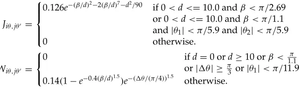
The self-excitatory connection isJo =0.8. The long-range synaptic con-nectionsJiθ,jθ0 andWiθ,jθ0 are determined as follows. Let the two edge
andθ2, where|θ1| ≤ |θ2| ≤π/2, andθ1,2are positive or negative depending
on whether the edges rotate clockwise or counterclockwise toward the con-necting line in no more than aπ/2 angle. Denoteβ=2|θ1| +2 sin(|θ1+θ2|),
1θ=θ−θ0with|θ−θ0| ≤π/2, then
Jiθ,jθ0 =
0.126e−(β/d)2−2(β/d)7−d2/90
if 0<d<=10.0 andβ < π/2.69 or 0<d<=10.0 andβ < π/1.1 and|θ1|< π/5.9 and|θ2|< π/5.9
0 otherwise.
Wiθ,jθ0 =
0 ifd=0 ord≥10 orβ < 1π.1
or|1θ| ≥π3 or|θ1|< π/11.999 0.14(1−e−0.4(β/d)1.5
)e−(1θ/(π/4))1.5
otherwise.
A.2 Derivation of the Connection Structure. We derive the qualitative structure of the neural connections, using the following computational re-quirements: (1) two nearby edge segments should enhance each other’s activities if one could draw a smooth contour passing both of them; (2) a small enough gap in a smooth contour of sufficient input length and strength should be filled by the network; (3) a smooth contour of finite length and width in input should not grow in length or width by the network enhance-ment.
According to equations 3.7 and 3.8, an edge segment(jθ0)can enhance or suppress edge segment(iθ)by sending monosynaptic excitatory input via connectionJiθ,jθ0or disynaptic inhibitory input via connectionWiθ,jθ0.
Hence, condition 1 above requiresJiθ,jθ0 6=0 if(iθ)and(jθ0)are nearby and roughly coaligned, as illustrated in Figure 4.
The bounds on the overall scale of theJconnection can be obtained by considering a contour of a straight line on the x-axis, as in equation 3.9. Omit theθvariables, let theith segment be atx=0, origin of the x-axis, and thejth the other contour segments. If only segmentiis missing in input, condition 2 requiresPjJijgx(xj) >Tx, or
P
jJij>Tx(forgx(xj)≤1). If segmentiand all segmentsjon the positive x-axis are missing in input, condition 3 requires
P
j<0Jij < Tx if the strong contour should be prevented to grow into the positive x-axis. These requirements, together with the contour reflection symmetryJij=Jji, constrain the overall scale ofJwithin a factor of 2.
However, a segment near and roughly parallel to the x-axis is excited by the coaligned contour segments on the x-axis and is likely to be filled by condition 2 since it provides an alternative route for the contour. To prevent such a straight contour from thickening, condition 3 requires disynaptic inhibition connectionsWiθ,jθ0connecting this segment from the nonaligned horizontal contour segments on the x-axis. AWconnection structure as in Figure 4 results; a lower bound on the overall scale of theWconnections can then be obtained.