Task management of Robot using Priority Job Scheduling

(1)

Task management of Robot using Priority Job

Scheduling

Amitava Kar*

1

, Ajoy Kumar Dutta

2

and Subir Kumar Debnath

2

1

Department of Computer Application, Asansol Engineering College, Asansol 2

Department of Production Engineering, Jadavpur University, Kolkata

Abstract— In this paper, we describe the application of priority scheduling in the field of robotics where a robot is assigned the work of picking up the jobs lying on the floor and to keep them in the given spaces. Priorities are assigned to each of the jobs and the robots are to pick up and complete the process of keeping it in the space according to the priorities of the jobs. The robot is connected to the cloud through a network. It is the cloud, who after calculation, tells about the places where the robot should go. The robot offloads the calculation of the distances of every job from it and the distances of the spaces from the jobs and the sequence of the jobs and the spaces where the jobs are to be kept. The cloud calculates the sequence of the jobs to be picked up by the robot and the location of the spaces where each job is to be kept. Cloud computing minimizes the need of the robot for high processor as the complex calculations are to be done in the cloud.

Keywords— Automated Robots, Cloud environment,

Queries, Priorities.

I. INTRODUCTION

The launching of the Internet in the 1990s led to the limited sharing of resources. The Cloud Computing is an application of such a resource sharing mainly software rather than a hardware. The hardware cannot be shared over the internet but load on the hardware can be reduced by offloading the storage to the cloud. The cloud is used not only for storage of large amount of data but also it relieves remote devices from the burden of carrying out extensive computations (Mell and Grance 2011). (Wen et al. 2011)spoke about energy optimal execution policy for a cloud-assisted mobile application platform. The calculations, if done on the Cloud, can save a lot of energy consumption for the cloud-assisted applications. It can then channelize its energy to some other activities. Cloud robotics uses the idea and includes the possibility of reducing the hardware requirement of a robot by storing the data in the cloud and getting them as and when required by querying them. It is fitted with a wifi system such that it can connect the cloud for storing data as well as for querying for data. It can also offload the complex calculations to the cloud and can query the result of the calculations as and when needed. This minimizes the hardware requirement (E.Guizzo 2011). (Arumugam et al. 2010) spoke about the application of Cloud Computing framework for service robots. (A.Kar et al. 2016a) spoke about the determination of the location of the task of the robot by the cloud. (A.Kar et al. 2016b) then spoke about the algorithms that may be followed for job scheduling by the cloud for the robot such

that the robot can perform its work moving the shortest possible distance.

II. METHODOLOGY OF WORK

The robot is assigned to pick up the jobs and keep them in a given spaces. The robot receives the coordinate of the job to be picked up and reaches the coordinate to pick up the job. It then receives the coordinate of the space where this job is to be kept. It reaches the space and keeps the job. The robot then

receives the coordinate of the next job to be picked up and it reaches the coordinate to pick up the next job and so on. Let us suppose that the name of the robot is R.

ASSUMPTIONS

 There are four jobs denoted by Js to be kept in the spaces containing six spaces denoted by Ss. So, some of the spaces may remain empty after the completion of the whole job.

 The jobs are scattered over the area.

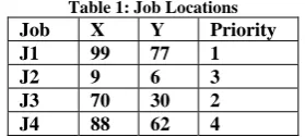
 Priorities are assigned to each jobs. The jobs are picked up according to their priorities. The priorities range from 1 to n, where 1 is the highest priority, followed by 2,3 and so on.

 Any job may be kept at any space.

 R(0,0) is the initial coordinate of the robot.

As the jobs are picked up, the location of the robot become the location of the jobs, that is just now picked up. As each job is kept in the space the location of the robot then becomes the location of the space, where the job is kept just now. This goes on till all the jobs are delivered. Two experiments were conducted and the datasets obtained were tested with the two algorithms discussed here.

Dataset-I

The coordinates of the points where the jobs are scattered are tabulated below:

Table 1: Job Locations

(2)

Let us also take the positions of the spaces where the jobs are to be arranged, are tabulated below:-

Table 2: Space Locations

Space X Y S1 0 100

S2 20 100

S3 40 100

S4 60 100

S5 80 100

S6 100 100

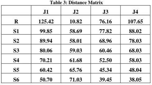
The cloud calculates the distance of the robot from its initial position to each of the jobs. It also calculates the distances of each of the jobs from each of the spaces. The distance matrix is given as under:-

Table 3: Distance Matrix

J1 J2 J3 J4 R 125.42 10.82 76.16 107.65 S1 99.85 58.69 77.82 88.02 S2 89.94 58.01 68.96 78.03 S3 80.06 59.03 60.46 68.03 S4 70.21 61.68 52.50 58.03 S5 60.42 65.76 45.34 48.04 S6 50.70 71.03 39.45 38.05

Algorithm - 1: Stage by Stage Shortest

Path

The maximum priority is J1, so R to J1 i.e. 125.42 is taken. The second maximum priority is J3. The distance from J1 to J3 via different spaces is given below in the table:

Table 4: J1 to J3 via Spaces

J1-J3 S1 177.67 S2 158.91 S3 140.53 S4 122.71 S5 105.76 S6 90.14

The route J1-S6-J3 is minimum. So it is chosen. The next priority is J2. The distance from J3 to J2 via different spaces is given in the table. S6 is already exhausted, so it is not in the table below:

J3-J2 S1 136.51 S2 126.97 S3 119.50 S4 114.18 S5 111.11

The route J3-S5-J2 is minimum. So it is chosen. The last job is J4. The distance from J2 to J4 via different spaces is given in the table. S5 is already exhausted, so it is not in the table below:

J2‐J4 S1 146.72 S2 136.03 S3 127.06

S4 119.72

The route J2-S4-J4 is minimum. So it is chosen. The J4 is to be kept in S1 or S2 or S3 spaces as all the other spaces are exhausted. J4 to different available spaces are given in the table below:

Table 7: J4 to available Spaces

J4 S1 88.02 S2 78.03 S3 68.03

The minimum is J4-S3. So it is chosen. The path is R-J1-S6-J3-S5-J2-S4-J4-S3 and the total distance is 125.42 + 90.14 + 111.11 + 119.72 + 68.03 = 514.42. The allocations are given in the table below:

Table 8: Jobs in Spaces

Jobs Spaces J1 S6 J3 S5 J2 S4 J4 S3

Algorithm - 2: Overall Shortest Path

In this algorithm the data are put in the same matrix. J1 has the highest priority and so R-J1 is chosen.

Table 9: Jobs and Spaces

J1-J3 J3-J2 J2-J4 J4 S1 177.67 136.51 146.72 88.02 S2 158.91 126.97 136.03 78.03 S3 140.53 119.50 127.06 68.03 S4 122.71 114.18 119.72 58.03 S5 105.76 111.11 113.81 48.04 S6 90.14 110.47 109.08 38.05

(3)

Table 10: J4-S6 is chosen

J1-J3 J3-J2 J2-J4 J4 S1 177.67 136.51 146.72 S2 158.91 126.97 136.03 S3 140.53 119.50 127.06 S4 122.71 114.18 119.72 S5 105.76 111.11 113.81

S6 38.05

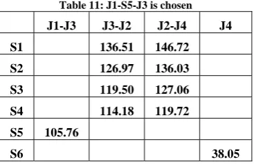
The next minimum is 105.76 which is the distances J1-S5-J3. It is chosen. Thus J1-J3 column and S5 row are exhausted.

Table 11: J1-S5-J3 is chosen

J1-J3 J3-J2 J2-J4 J4

S1 136.51 146.72

S2 126.97 136.03

S3 119.50 127.06

S4 114.18 119.72

S5 105.76

S6 38.05

The next minimum is 114.18 which is the distance J3-S4-J2. It is chosen. Thus J3-J2 column and S4 row are exhausted.

J1-J3 J3-J2 J2-J4 J4

S1 146.72

S2 136.03

S3 127.06

S4 114.18 S5 105.76

S6 38.05

The next minimum is 127.06 which is the distance of J2-S3-J4. It is chosen.

J1-J3 J3-J2 J2-J4 J4 S1

S2

S3 127.06

S4 114.18 S5 105.76

S6 38.05

The route thus becomes R-J1-S5-J3-S4-J2-S3-J4- S6 and the total distance is 125.42+105.76+114.18+ 127.06 + 38.05 = 510.48 The allocations are given in the table below:

Table 14: Jobs in Spaces Jobs Spaces

J1 S5

J3 S4

J2 S3

J4 S6

Dataset-II

The coordinates of the points where the jobs are scattered are tabulated below:

Table 15: Job Locations

Job X Y Priority J1 56 88 P4 J2 76 68 P3 J3 50 58 P1 J4 40 19 P2

Let us also take the positions of the spaces where the jobs are to be arranged, are tabulated below:

Table 2: Space Locations

Space X Y S1 0 100

S2 20 100

S3 40 100

S4 60 100

S5 80 100

S6 100 100

The cloud calculates the distance of the robot from its initial position to each of the jobs. It also calculates the distances of each of the jobs from each of the spaces. The distance matrix is given as under:

Table 17: Distance Matrix

(4)

Algorithm - 1: Stage by Stage Shortest

Path

The maximum priority is J3, so 76.58 is taken. The second maximum priority is J4. The distance from J3 to J4 via different spaces is given below in the table:

J3-J4 S1 155.64 S2 135.05 S3 124.17 S4 126.61 S5 141.95 S6 166.10

The route J3-S3-J4 is minimum. So it is chosen.

The next priority is J2. The distance from J4 to J2 via different spaces is given in the table. S3 is already exhausted, so it is not in the table below:

J4-J2 S1 172.80 S2 147.93 S4 119.21 S5 122.59 S6 140.80

The last job is J1. The distance from J2 to J1 via different spaces is given in the table. S3 and S4 is already exhausted, so it is not in the table below:

J2-J1 S1 139.73 S2 102.45 S5 59.08 S6 85.61

The J1 is to be kept in S1 or S2 or S6 spaces as all the other spaces are exhausted. J1 to different available spaces are given in the table below:

Table 21: J1 to available Spaces

J1 S1 57.27 S2 37.95 S6 45.61

The minimum is J1-S2. So it is chosen. The path is R-J3-S3-J4-S4-J2-S5-J1-S2. The total distance is

76.58+124.17+119.21+59.08+37.95 = 416.99. The jobs kept in spaces are given in the table below:

Algorithm - 2: Overall Shortest Path

In this algorithm the data are put in the same matrix. J3 has the highest priority and so R-J3 is chosen.

Table 23: Jobs and Spaces

VIA J3-J4 J4-J2 J2-J1 J1 S1 155.64 172.80 139.73 57.27 S2 135.05 147.93 102.45 37.95 S3 124.17 129.17 68.17 20.00 S4 126.61 119.21 48.43 12.65 S5 141.95 122.59 59.08 26.83 S6 166.10 140.80 85.61 45.61

The minimum is 12.65 which is the distance J1 and S4. So it is chosen. S4 is thus the last space in the route where J1 is to be kept. The corresponding J1- column and S4 row are exhausted.

Table 24: J1-S4 is chosen

VIA J3-J4 J4-J2 J2-J1 J1 S1 155.64 172.80 139.73 S2 135.05 147.93 102.45 S3 124.17 129.17 68.17

S4 12.65

S5 141.95 122.59 59.08 S6 166.10 140.80 85.61

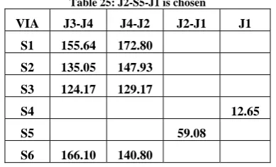
The next minimum is 59.08 which is the distance J2-S5-J1. It is chosen. Thus J2-J1 column and S5 row are exhausted.

VIA J3-J4 J4-J2 J2-J1 J1 S1 155.64 172.80

S2 135.05 147.93 S3 124.17 129.17

S4 12.65

S5 59.08

S6 166.10 140.80

(5)

VIA J3-J4 J4-J2 J2-J1 J1 S1 172.80 S2 147.93 S3 124.17

S4 12.65

S5 59.08

S6 140.80

The next minimum is 140.80 which is the distance of J4-S6-J2. It is chosen.

VIA J3-J4 J4-J2 J2-J1 J1

S1

S2

S3 124.17

S4 12.65

S5 59.08

S6 140.80

The route thus becomes R-J3-S3-J4-S6-J2-S5-J1-S4 and the total distance is 76.58+124.17+140.80+59.08+ 12.65 = 413.28

The allocations are given in the table below:

III. COMPARISONS OF THE TWO ALGORITHMS Of the two algorithms discussed above, the distance to be covered by the robot for doing the whole job in the

Algorithm-I is 514.42 whereas in case of the Algorithm-II it is 510.48. This is for the Dataset-I.

Figure 2: Comparison of the total distances traveled for Algorithm-I and Algorithm-II for Dataset-I

The distance covered for Algorithm-I is 416.99 which is again more than 413.28, the distance covered for Algorithm-II in case of Dataset-II. It may be shown that the total distance covered in case of Algorithm-II will always be less than the total distance covered in case of Algorithm-I because it considers the matrix as a whole. But the time complexity of I is better than that of Algorithm-II. Figure-2 for Dataset-I and Figure-3 for Dataset-II shows clearly that the distance covered in Algorithm-I is slightly more than that of Algorithm-II.

Figure 3: Comparison of the total distances traveled for Algorithm-I and Algorithm-II for Dataset-II

The time complexity of Algorithm - I: If there are m jobs and n spaces where m<n, the time complexity of this algorithm is O(mn) ≈ O(n2_).

The time complexity of Algorithm-II: If there are m jobs and n spaces where m<n, the time complexity of finding the minimum of the matrix takes O(mn)time ≈ O(n2_{) time for}

each job. For m jobs it is t O(n3). But it can guarantee a result better than the 1st algorithm in terms of total distance covered for completing all the jobs.

Had the calculation been done by the robot, the Algorithm-II would have wasted too much energy and time of the robot as compared to Algorithm-I and it would have led to starvation of a number of processes and might also lead to deadlock, but all the calculations are done by the cloud and so higher time

complexity do not have any effect on the robot as the robot only queries about the location where it is to go and reaches that location and lifts the job and then again queries about the location where it is to reach and reaches that destination and keeps the job in that location.

IV. CONCLUSION

(6)

calculation purpose is also minimized as it does not need to do any calculations. It can get the result of any calculations from the cloud. The reduction for the need of high memory capacity and high processor for calculation may lead to reduction of the complexity of the processes running inside the robot. It may reduce the situations of process starvation and process deadlock and may reduce the price of the robot.

REFERENCES

[1] A.Kar, A. K. Dutta, and S. K. Debnath (2016a).Determining the location of the tasks of robotby the cloud. International Journal of Advanced Information Science and Technology 54, 20-25. [2] A.Kar, A. K. Dutta, and S. K. Debnath (2016b).Task management of

robot using cloud computing. IEEE International Conference on Computer, Electrical and Communication Engineering, 2016. [3] Arumugam, R., V. R. Enti, L. Bingbing, W. Xi-aojun, K. Baskaran,

F. F. Kong, A. S. Kumar, K. D. Meng, G. Kit, M. Rakotondrabe,and I. Ivan (2010).

[4] Davinci: A cloud computing framework for service robots. International Conference on Robotics and Automation , 3084-3089. [5] E.Guizzo (2011). Robots with their heads in the clouds. IEEE

Spectrum

[6] .Mell, P. and T. Grance (2011). The nist de_nition of cloud computing. National Institute of Standards and Technology Special Publication 800,

[7] Wen, Y., W. Zhang, K. Guan, D. Kilper, and H. Luo (2011). Energy-optimal execution policy for a cloud-assisted mobile application platform. NTU Technical Report .

AUTHORS PROFILE

Dr. Ajoy Kumar Dutta is currently a Professor in the

Department of Production Engineering, Jadavpur University, INDIA. He received his B. E. & M. E. degrees in Electronics & Tele-communication Engg from Jadavpur University in 1983 & 1985 respectively, and Ph. D. (Engg) degree in the area of Robotics from Jadavpur University in 1991. His Field of Specialization and Research Area are Robotics, Sensors, Computer Vision, Microprocessor Applications, and Mechatronics. He has teaching & research experience of 31 years.

Mr. Subir Kumar Debnath is currently an Associate Professor in the Department of Production

Engineering, Jadavpur University, INDIA. He received his B. E. degree in Mechanical Engg from Jadavpur University in 1982 & M. Tech in Mechanical Engg in 1984 from I.I.T.- Kharagpur, INDIA. His Field of Specialization and Research Area are Robotics, Sensors, Computer Vision, CNC Machines and Automation. He has teaching & research experience of 31 years.

Mr. Amitava Kar is currently an Assistant Professor