Lattice Decoding Attacks on Binary LWE
Shi Bai and Steven D. Galbraith Department of Mathematics,
University of Auckland, New Zealand. [email protected] [email protected]
Abstract. We consider the binary-LWE problem, which is the learn-ing with errors problem when the entries of the secret vector are chosen from{0,1}or{−1,0,1}(and the error vector is sampled from a discrete Gaussian distribution). Our main result is an improved lattice decod-ing algorithm for binary-LWE which first translates the problem to the inhomogeneous short integer solution (ISIS) problem, and then solves the closest vector problem using a re-scaling of the lattice. We also dis-cuss modulus switching as an approach to the problem. Our conclusion is that binary-LWE is easier than general LWE. We give experimental results and theoretical estimates that can be used to choose parameters for binary-LWE to achieve certain security levels.
Keywords:lattice decoding attacks, learning with errors, closest vector problem.
1
Introduction
The learning with errors problem is: Given an m×n matrix A and a vector
b≡As+e (mod q), wheree∈Zmq is a “short” error vector, to computes∈Znq.
This is a computational problem of major current importance in cryptography. Recently, Brakerski, Langlois, Peikert, Regev and Stehl´e [8] and Micciancio and Peikert [21] have considered variants of this problem where the secret vectors are chosen uniformly from the set{0,1}n (or{−1,0,1}n), rather than from
Znq.
These variants of the problem are called binary-LWE.
It is natural to expect that the binary-LWE problem is easier than the stan-dard LWE problem, but it is an open question to determine how much easier. Both papers [8, 21] give reductions that imply that binary-LWE is hard, but those results require increasing the parameter n to approximately nlog2(q) = O(nlog2(n)) (it is usually the case thatq is a low-degree polynomial inn). An interesting problem is to determine whether these results are optimal. As an ex-ample, taking n= 256 for standard LWE would lead to a parameter of at least nlog2(n) = 2048 for binary LWE, which seems excessive.
lattice so that the standard lattice methods to solve the closest vector problem are more effective. We also consider other approaches to the problem, such as modulus switching. We show that modulus switching is not a helpful tool in this setting, which may be counter-intuitive. We also give theoretical and experimen-tal analysis of the algorithm.
Experimental results with the new algorithm do confirm that the parameter n needs to be increased when using binary-LWE. Returning to the example of n= 256, our results suggest that a parameter around 440 may be sufficient to achieve the same security level as standard LWE with parameter 256. This is much smaller and therefore more practical than using parameter 2048.
Our approaches are all based on lattice decoding attacks. There is another class of algorithms for LWE that are more combinatorial, originating with Blum, Kalai and Wasserman [6, 1]. However, these algorithms require an extremely large number of samples from the LWE distribution, which may not be realistic in certain applications.
The paper is organised as follows. Sections 2 and 3 give precise definitions for the LWE and binary-LWE problems. Section 4 recalls the current state-of-the-art for lattice attacks on LWE. Section 5 describes modulus switching and evaluates its performance. Section 6 contains our algorithm and its analysis, specifically the description of the rescaling in Section 6.1 and the discussion of why modulus switching is unhelpful in Section 6.3. Some experimental results, that confirm our improvement over previous methods, are given in Section 7.
2
LWE
Let σ ∈R>0. Define ρσ(x) = exp(−x2/(2σ2)) and ρσ(Z) = 1 + 2P∞x=1ρσ(x).
The discrete Gaussian distribution Dσ on Z with standard deviation σ is the distribution that associates tox∈Zthe probabilityρσ(x)/ρσ(Z).
Fix parameters (n, m, q, σ). Typical choices of parameters are (n, m, q, σ) = (256,640,4093,32). Let A be a uniformly chosen m×n matrix with entries in Zq. Let s and e be integer vectors of lengths n and m respectively whose
entries are sampled independently from the Gaussian distribution on Z with standard deviationσ(this is the case of LWE with secrets chosen from the error distribution, which is no loss of generality [3]). We callsthe “secret vector” and
e the “error vector”. The LWE distribution is the distribution on (Zm×n
q ,Zmq )
induced by pairs (A,b≡As+e (mod q)) sampled as above. The search-LWE problem is: Given (A,b) chosen from the LWE distribution, to compute the pair (s,e). The search-LWE problem is well-defined if there is one pair (s,e) satisfyingb≡As+e (mod q) that is significantly more likely (with respect to the distributions on (s,e)) to have be chosen than any other solution.
The (m, n, q,B)-SIS problem is: Given an n×m integer matrix A0 (where typically m is much bigger than n) and an integerq to find a vector y ∈Zm,
if it exists, such that A0y≡ 0 (modq) and y∈ B. Here B is a set of vectors that are “short” in some sense (e.g., B={y∈Zm:kyk ≤B} for some bound
SIS problem (ISIS): Given A0 andv findy∈ B, if it exists, such that A0y≡v
(mod q).
The LWE problem can be rephrased as inhomogenous-SIS: Given (A,b≡ As+e (modq)) one can form the ISIS instance
(A|Im)
s e
≡b (mod q)
whereImis them×midentity matrix. An alternative transformation of LWE to
ISIS is mentioned in Remark 1 of Section 4.3. Conversely, ISIS can be translated to LWE, for details see Lemmas 9 and 10 of Micciancio and Mol [20]. However, it is notable that the (I)SIS problem has often been considered in the case when the solution vectorymight lie in{0,1}mor{−1,0,1}mand might not be uniquely
determined, whereas for LWE the focus has always been on vectors sampled from discrete Gaussians and there being a unique most likely solution.
2.1 Size of the error vector
Let Dσ be the discrete Gaussian distribution on Z with standard deviation σ. Let e be sampled from Dmσ, which means that e = (e1, . . . , em) is formed by
taking m independent samples from Dσ. We need to know the distribution of
kek. If the entriesei were chosen from a true Gaussian with standard deviation
σ then kek2 comes from the chi-squared distribution, and so has mean mσ2. Since our case is rather close, we assume thatkek2 is also close to a chi-squared distribution, and we further assume that the expected value of kek is close to
√
mσ. Lyubashevsky (Lemma 4.4(3) of the full version of [18]) shows that
Pr kek ≤kσ√m
≥1−ke1−k 2 2
m
for k > 0. This supports our assumption that kek ≈ √mσ. To achieve over-whelming probability, we may use k≈2. In practice, this bound is quite useful fork'1. In practice, we can easily estimate the expected value of kek for any fixed parameters by sampling.
3
Binary LWE and related work
We now restrict the LWE problem so that the secret vectorsis chosen to lie in a much smaller set. Fix (n, m, q, σ). To be compatible with Regev’s results (e.g., see Theorem 1.1 of [24]), we usually takeσ≈2√n. LetAbe a uniformly chosen m×nmatrix with entries inZq. Lets∈Zn have entries chosen independently and uniformly from {0,1}. Let e ∈ Zm have entries sampled independently
from the discrete Gaussian distribution on Z with standard deviation σ. The binary-LWE distribution is the distribution on (Zm×n
q ,Zmq ) induced by pairs
(s,e). One can also consider a decisional problem, but in this paper we focus on the search problem.
The binary-LWE problem (where secret vectorssare from{0,1}n) has been
considered in work by Brakerski, Langlois, Peikert, Regev and Stehl´e [8]. The main focus of their paper is to prove hardness results for LWE in the classical setting (i.e., without using quantum algorithms as in Regev’s original result). They use modulus switching, which is a tool to transform an LWE instance moduloqto an LWE instance modulo a different primeq0. Micciancio and Peik-ert [21] have considered the binary-LWE problem where s∈ {−1,0,1}n. Their
main result is a hardness result for the case where not only the secrets are small but even the errors are small. Of course, due to the Arora-Ge attack [4] this is only possible if one makes the (realistic) assumption that one has access to a very restricted number of samples from the LWE distribution. This problem is closely relevant to the ISIS problem, since the ISIS problem is always stated in terms of a fixed number of samples.
It is worth noting that there is a standard reduction [3] from LWE to the case of LWE where the secret is chosen from the error distribution. But there is not a general reduction from LWE instances to ones whose error is chosen from the secret’s distribution (apart from the naive case ofn×nLWE instances (A,b≡ As+e (modq)) giving (A0 ≡ A−1 (modq),b0 ≡ A−1b ≡ A0e+s
(mod q)) ).
Both papers [8, 21] give reductions that imply that binary-LWE is hard, as-suming certain other lattice problems are hard. Essentially, the papers relate (n, q)-binary-LWE to (n/t, q)-LWE (wheret=O(log(n)) =O(log(q))). In other words, we can be confident that binary-LWE is hard as long as we increase the parameternby a factor of log(n). For example, taking n= 256 as a reasonably hard case for standard LWE, we can be confident that binary-LWE is hard for n= 256 log2(256) = 2048. Our feeling is that these reductions are too conserva-tive, and that binary-LWE is harder than these results would suggest.
The main goal of our paper is to study the LWE problem where the secret vector is binary, but the errors are still discrete Gaussians. We focus on the case s ∈ {−1,0,1}n, but our methods are immediately applicable to the case
s∈ {−B, . . . ,−1,0,1, . . . , B} for anyB < σ.
It is clear that one can solve the binary-LWE problem inO(3n) operations (or O(2n) when entries are in{0,1}), by trying all choices forsand testing whether
b−As (modq) is a short vector. There is also a meet-in-the-middle attack that requires ˜O(3n/2) (respectively, ˜O(2n/2)) space and time. One can also convert to ISIS and apply algorithms due to Howgrave-Graham and Joux [13] and Becker, Coron and Joux [5]. All such attacks can be defeated by taking n≥ 200 (the storage requirement is a serious constraint).
4
Standard lattice attack on LWE
Typically the rank ofAwill ben, and soLhas volumeqm−n. Suppose one can
solve the closest vector problem (CVP) instance (L,b). Then one finds a vector
v∈L such thatkb−vk is small. Writinge=b−v andv≡As (mod q) for some s∈Zn (it is easy to solve forsusing linear algebra whenm≥n), then
b≡As+e (mod q).
Hence, if we can solve CVP then we have a chance to solve LWE.
The CVP instance can be solved using the embedding technique [14] (reduc-ing CVP to SVP in a lattice of dimension one larger) or an enumeration algo-rithm (there are several such algoalgo-rithms, but Liu and Nguyen [16] argue that all variants can be considered as cases of pruned enumeration algorithms). For the complexity analysis here we use the embedding technique, so we recall this now. Some discussions of enumeration algorithms will be given in Section 7.3.
Let L ⊆ Zm be a lattice of rank m with (column) basis matrix B, and suppose b ∈ Zm is a target vector. We wish to find v = Bu ∈ L such that
e=b−v=b−Buis a short vector. The idea is to consider the basis matrix, whereM ∈Nis chosen appropriately (e.g.,M ≈
√
mσ),
B0=
B b
0 M
. (1)
This is the basis for a latticeL0 of rankd=m+ 1 and volumeM·vol(L). Note that
B0
−u
1
=
−Bu+b
M
=
e
M
.
Hence, the (column) lattice generated by B0 contains a short vector giving a potential solution to our problem. One therefore applies an SVP algorithm (e.g., LLL or BKZ lattice basis reduction).
Lyubashevsky and Micciancio (Theorem 1 of [17]) argue that the best choice forM above iskek, which is approximately√mσin our case. However, in our experiments M = 1 worked fine (and leads to a more powerful attack [2] in practice).
4.1 Unique-SVP
Gama and Nguyen [11] have given a heuristic approach to estimate the capability of lattice basis reduction algorithms. Consider a lattice basis reduction algorithm that takes as input a basis for a lattice Lof dimension d, and outputs a list of vectorsb1, . . . ,bd. Gama and Nguyen define the root Hermite factor of such an
algorithm to beδ∈Rsuch that
kb1k ≤δdvol(L)1/d for alldand almost all latticesL.
using extreme pruning and large block size). Chen and Nguyen [10] extended this analysis to algorithms with greater running time. Their heuristic argument is that a Hermite factor corresponding toδ= 1.006 might be reachable with an algorithm performing around 2110operations.
In Section 3.3 of [11], Gama and Nguyen turn their attention to the unique-SVP problem. One seeks a short vector in a lattice L when one knows that there is a large gap γ =λ2(L)/λ1(L), where λi(L) denotes the i-th successive
minima of the lattice. The unique-SVP problem arises when solving CVP using the embedding technique. The standard theoretical result is that if one is using a lattice reduction algorithm with Hermite factorδ, then the algorithm outputs the shortest vector if the lattice gap satisfies γ > δ2m. However, Gama and
Nguyen observe that practical algorithms will succeed as long as γ > cδm for
some small constant c (their paper gives c = 0.26 and c = 0.45 for different families of lattices). Moreover, Luzzi, Stehl´e and Ling [19] gave some theoretical justification that the unique-SVP problem is easier to solve when the gap is large.
4.2 Application to LWE
Consider running the embedding technique on an LWE instance, using the lattice L0 given by the matrixB0 from equation (1). We have a good chance of getting the right answer if the error vector e is very short compared with the second shortest vector in the lattice L0, which we assume to be the shortest vector in the original lattice L.
The Gaussian heuristic suggests that the shortest vector in a latticeLof rank d has Euclidean norm about √1
πΓ(1 +
d
2)
1/dvol(L)1/d which is approximately q
d
2πevol(L)
1/d. In latticeL (of rankm), this is p m
2πeq
(m−n)/m. Note also that
our lattices contain known vectors of Euclidean length equal to q. Hence, our estimate of the Euclidean length of known short vectors is
λ2(L0)≈λ1(L)≈min
q,
r
m 2πeq
m−n m
.
In contrast, the vectorehas Euclidean length around √mσon average (see Section 2.1), and so the vector (Me) has length approximately√2mσwhenM =
√
mσ. In our experiments we takeM = 1 and so assume that λ1(L0)≈
√
mσ. Hence the gap is
γ(m) = λ2(L 0) λ1(L0)
≈ min{q,
1 √
πΓ(1 +
m
2)
1/mqmm−n}
√
mσ ≈
min{q,p m
2πeq
m−n m }
√
mσ . (2)
For a successful attack we want this gap to be large, so we will need
To determine whether an LWE instance can be solved using the embedding technique and a lattice reduction algorithm with a given (root) Hermite factor δ, one can choose a suitable subdimension mand verify that the corresponding gap satisfies the condition γ = γ(m) > cδm for a suitable value c. Since the
constant c is unknown, we can maximize min{q, q(m−n)/m}/δm for fixedn, q, δ
to get the “optimal” sub-dimension (which maximizes the success probability of the algorithm) to be
m=
s
nlog(q)
log(δ) , (3)
whereδ is the Hermite factor of the lattice basis reduction algorithm used. Furthermore, we may assume c is upper bounded by 1 due to Gama and Nguyen [11]. Hence, for fixedn, q, σ= 2√n, we can easily compute values (m, δ) satisfying the constraint γ1/m ≥ δ and such that δ is maximal. These values
have lattice dimensionmas in equation (3). By doing this we obtained Table 1 (forn≥160 the length of the second shortest vector is taken to beq and this leads to very large dimensions; enlargingqto around 13000 in the casen= 300 leads tom= 1258 andδ≈1.002). The last row consists of the estimated time
log(TBKZ) =
1.8
log2(δ)−110 (4)
for running the BKZ lattice basis reduction algorithm, based on Lindner and Peikert’s work [15]. Note that we do not know the value of the constant c for our lattices, only the experimental results by Gama and Nguyen [11]. There is no known sharp theoretical bound for it. Hence the running time in Table 1 may not be the optimal embedding attack for the LWE problem with parametern.
Table 1: Theoretical prediction of (optimal) root Hermite factor δ and running time
T of the standard embedding technique algorithm using BKZ for LWE instances with
q = 4093,σ = 2√n for the given values forn. The lattice dimension d =m+ 1 is calculated using equation (3) and the running timeT is estimated using equation (4).
n 30 40 50 60 70 100 150 200 250 300
d 110 151 194 239 284 425 673 1144 1919 3962
δ≈ 1.0208 1.0147 1.0111 1.0088 1.0072 1.0046 1.0028 1.0013 1.0006 1.0002 log(T)≈ 0 0 3 33 63 161 343 872 2100 7739
4.3 How to solve ISIS
Recall the inhomogeneous-SIS (ISIS) problem: Given (A0,v) to find a short vector y ∈ Zm such that v ≡ A0y (mod q). It is standard that ISIS is also attacked by reducing to CVP: One considers the lattice L0 =Λ⊥
q(A
0) =
{y ∈
Zm :A0y≡0 (modq)}, finds any vector (not necessarily short) w∈Zm such that A0w≡v (modq), then solves CVP for (L0,w) to find somey close tow
and so returnsw−yas the ISIS solution.
We sketch the details of solving LWE (in the case of short secrets) by reducing to ISIS and then solving by CVP (more details are given in Section 6). Given (A,b) we defineA0= (A|Im) to get an ISIS instance (A0,b). Choose any vector
w∈Zn+m such that A0w≡b (modq). Then the lattice L0 =Λ⊥q(A0) ={y∈
Zn+m:A0y≡0 (modq)} is seen to have rankm0 =n+m and (assuming the rank of A0 is n) determinant qm = qm0−n (the determinant condition can be
seen by considering the index of the subgroupqZn+min the additive groupL0). The condition for success in the algorithm isσqm/(n+m). Writingm0=n+m this isq(m0−n)/m0, which is the same as the LWE condition above.
Remark 1. We can also reduce LWE to ISIS using the approach of Micciancio and Mol [20]. In particular, one can construct a matrix A⊥ ∈Z(qm−n)×m such
thatA⊥A≡0 (modq). The LWE problem (A,b) is therefore transformed into the ISIS instance (A⊥,A⊥b≡A⊥e (modq)). It follows that a solution to the ISIS problem gives a value for eand hence solves the LWE problem. It is easy to see that this approach is equivalent to the previous one in the case where the secret vector s is chosen from the error distribution. However, since this reduction eliminates the vectors, we are no longer able to take advantage of the “smallness” ofscompared withe, as we will do in the following sections. So we do not consider this approach further.
4.4 Distinguishing attack
One can also study the decisional variant of the LWE problem: Given a pair (A,b) to decide if it has been sampled uniformly at random fromZm×n
q ×Zmq ,
or from the LWE distribution. There is a standard distinguishing algorithm based on finding short vectors in the lattice {v∈Zm:vA≡0 (modq)}. The idea is
that ifvis such a lattice point and ifb≡As+e (mod q) thenvb≡ve (mod q) may be a small integer. Linder and Peikert [15] have argued that this approach is generally less effective than the decoding attack on the computational variant of LWE. We remark that one can define a decisional variant of binary-LWE (where the LWE distribution is defined by choosing bothsandeto be small), but the above distinguishing attack no longer solves this problem as it only tests thate
is small. Hence, we do not consider the distinguishing attack in this paper.
5
Modulus switching
(mod q)) as
b=As+e+qu
for some u∈Zm. Now supposeq0 is another integer and defineA0= [q
0
qA] and
b0= [qq0b], where the operation [ ] applied to a vector or matrix means rounding each entry to the nearest integer. WriteA0= qq0A+Wandb0 =qq0b+wwhere
W is anm×nmatrix with entries in [−1/2,1/2] and w is a lengthm vector with entries in [−1/2,1/2]. One can now verify that
b0−A0s= qq0b+w−(qq0A+W)s
= qq0(As+e+qu−As) +w−Ws
= qq0e+w−Ws+q0u.
One sees that (A0,b0) is an LWE instance moduloq0, with the same secret vector, and that the “error vector” has length
kqq0e+w−Wsk ≤ qq0kek+kwk+kWsk.
Note that the final term kWsk has the potential to be small only when shas small entries, as is the case for binary LWE. The termkwkis bounded by 12√m. The termkWskis easily bounded, but it is more useful to determine its expected value. Each entry of the vectorWsis a sum ofn(or aroundn/2 in the case where
s∈ {0,1}n) rational numbers in the interval [−1/2,1/2]. Assuming the entries of
Ware uniformly distributed then the central limit theorem suggests that each entry of Ws has absolute value roughly 1
4
p
n/2. Hence, it seems plausible to think thatkWskcan be as small as 14√nm.
Modulus switching was originally proposed to control the growth of the noise under homomorphic operations. The standard scenario is that if kek becomes too large then, by taking q0 much smaller thanq, one can reduce the noise by the factor qq0 while only adding a relatively small additional noise. However, the idea is also interesting for cryptanalysis: One can perform a modulus switching to make the error terms smaller and hence the scheme more easily attacked. We will consider such an attack in the case of binary LWE in the next section.
We now give a back-of-the-envelope calculation that shows modulus switch-ing can be a useful way to improve lattice attacks on LWE. Note that modulus switching reduces the error vector by a factor of qq0, as long as the other terms (dominated by 14√nm) introduced into the noise are smaller than qq0σ√m. How-ever, note that the volume of the lattice is also reduced, since it goes from q(m−n)/mto q0(m−n)/m. Let us writefor the reduction factor q0
q. All other
pa-rameters remaining the same, the lattice gap γ=λ2/λ1 ≈q(m−n)/m/(σ√2πe) changes to
Now, 0< < 1 and so this is a positive improvement to the lattice gap (and hence the Hermite factor).
For LWE we usually have errors chosen from a discrete Gaussian with stan-dard deviation at most 2√n, and so kek is typically O(√mn). As discussed above, the additional noise introduced by performing modulus reduction (from theWsterm) will typically be around 1
4
√
nm. Hence, it seems the best we can hope for is q0/q≈ 1
8 giving an error vector of norm reduced by a factor of ap-proximately 14 (from 2√mn to√mn/2). This does give a modest improvement to the performance of lattice decoding algorithms for LWE.
6
New attacks on binary-LWE
We now present our original work. We want to exploit the fact thatsis small. The standard lattice attack on LWE (reducing to CVP) cannot use this information. However, going via ISIS seems more appropriate.
6.1 Reducing binary-LWE to ISIS and then rescaling
Let (A,b) be the (n, m, q, σ)-LWE instance. We may discard rows to reduce the value form. We writem0=n+m. WriteA0= (A|Im), being anm×m0matrix,
and consider the ISIS instance
b≡A0(se) (modq) where the target short vector is (s
e).
The next step is to reduce this ISIS instance to CVP in a lattice. So define the vector w= (0,bT)T. Clearly A0w≡b (mod q). We now construct a basis matrixB for the latticeL0 ={v∈Zm
0
:A0v≡0 (modq)}. This can be done as follows: The columns of the (n+m)×(m+ 2n) matrix
M=
In
qIn+m
−A
span the space of all vectors v such that A0v ≡ 0 (modq). Computing the column Hermite normal form ofM gives anm0×m0 matrixB whose columns generate the latticeL0.
One can confirm that det(B) = qm = qm0−n. As before, we seek a vector
v∈Zm
0
such thatBv≡0 (modq) andv≈w. We hope thatw−v= (es) and so v= (∗s), where∗ is actually going to beb−e. Our main observation is that
ksk kekand so the CVP algorithm is trying to find an unbalanced solution. It makes sense to try to rebalance things.
Hermite factor of the problem is increased and hence the range of the lattice attack for a given security level is increased.
A further trick, whens ∈ {0,1}n, is to rebalance sso that it is symmetric
around zero. In this case we rescale by multiplying the firstnrows of Bby 2σ and then subtract (σ, . . . , σ,0, . . . ,0)T from w. Now the difference w−v is of
the form
(±σ, . . . ,±σ,e1, . . . ,em)T
which is more balanced.
6.2 Gap in the Unique-SVP
The determinant has been increased by a factor of σn (or (2σ)n in the {0,1}
case). So the gap in the re-scaled lattice is expected to be larger compared to the original lattice. In the embedded lattice formed by the standard attack, λ1(L0)≈√m·σandλ2(L0)≈q(m−n)/mpm
2πe wheremis the subdimension being
used. In the embedded lattice formed by the new attack, λ1(L0)≈√m+n·σ and λ2(L0) ≈ (qmσn)1/(m+n)
q m+n
2πe where m is the number of LWE samples
being used. Hence the new lattice gap isγ=λ2(L0)/λ1(L0) and so we will need to use lattice reduction algorithms with Hermite factorδ≤γ1/(m+n).
Lemma 1. Let q, n, σ and δ be fixed. Letm0 ≈m+n be the dimension of the embedded lattice in the new attack. For a given Hermite factor δ, the optimal value for m0 is approximately
s
n(logq−logσ)
logδ . (6)
Proof. The goal is to choosem0(and hencem) to minimize the functionf(m0) = q(m0−n)/m0σn/m0δ−m0. It suffices to find a minimum for the function F(x) =
log(f(x)) = ((x−n)/x) log(q) + (n/x) log(σ)−xlog(δ). Differentiating gives n(log(q)−log(σ)) =x2log(δ) and the result follows.
Table 2: Theoretical prediction of (optimal) root Hermite factorδand running timeTof embedding technique for rescaled binary-LWE instancess∈ {−1,0,1}nwithq= 4093,
σ= 2√nfor the given values forn. The lattice dimensiond0(≈m0) is calculated using equation (6) and the running timeT is estimated using equation (4).
n 30 40 50 60 70 100 150 200 250 300
d0 78 105 132 160 187 271 414 558 799 1144
δ 1.0296 1.0212 1.0164 1.0132 1.0111 1.0073 1.0045 1.0032 1.0019 1.0011
log(T) 0 0 0 0 3 63 169 280 545 1031
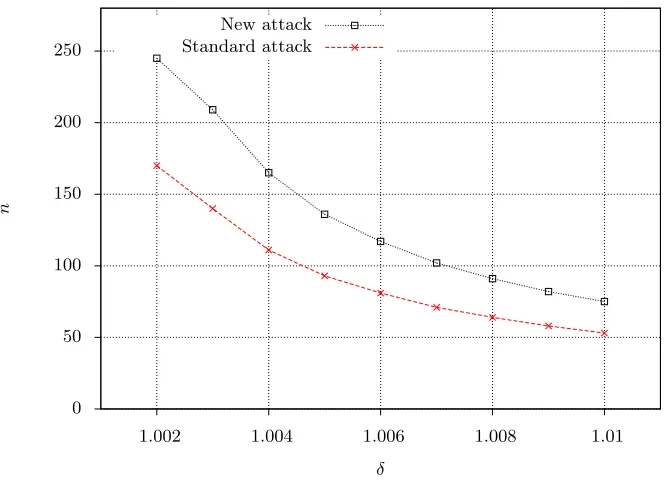
0 50 100 150 200 250
1.002 1.004 1.006 1.008 1.01
n
δ
New attack Standard attack
Fig. 1: Theoretical prediction of the largest binary-LWE parameternthat can be solved using an algorithm with the given root Hermite factor.
By fixing a lattice reduction algorithm that has the ability to produce some fixed Hermite factorδ, we can compare the maximumnthat this algorithm can attack, based on the standard attack or our new attack. Figure 1 indicates that, for instance, the binary LWE with secret in {−1,0,1} and n ≈ 100 provides approximately the same security as the regular LWE with n≈70.
6.3 Using modulus switching
It is natural to consider applying modulus switching before performing the im-proved lattice attack. We now explain that this is not a good idea in general.
As discussed in Section 5, the best we can try to do is to have q0/q ≈1/8 and the error vector is reduced in size from elements of standard deviationσto elements of standard deviation approximatelyσ/4.
Consider the desired Hermite factorδ=γ1/m0 to attack a lattice with gap
γ= (σn/m0q(m0−n)/m0/(σ√2πe))1/m0
as in our improved lattice attack using rescaling. Applying this attack to the lattice after modulus switching gives Hermite factor
(1 4σ)
n/m0(1 8q)
(m0−n)/m0/(1 4σ
√
2πe) 1/m0
=δ
1
2(m0−n)/m0 1/m0
which is strictly smaller than δ. Hence, the instance after modulus switching is harder than the instance before modulus switching. Intuitively, the problem is this: Modulus switching reduces the size of q and also the size of the error. But it reducesq by a larger factor than it reduces the size of the error (due to the additional error arising from the modulus switching process). When we do the rescaling, we are also rescaling by a smaller factor relative to q. Hence, the crucial lattice gap property is weakened by modulus switching.
6.4 Combining the lattice attack with exhaustive search
A natural extension is to first guess k bits of the secret s and then apply the lattice attack to the remaining problem. Since this reducesnit also reduces the optimal choice form, leading to a simpler problem.
For example, attacking an instance withn= 100 one could repeat the attack 225 times, trying all possibilities for the first 25 entries of s, where the lattice attack is now applied to binary-LWE instances havingn= 75, which seems quite practical compared with the 264 time for n= 100 predicted in Table 2. We do not consider this further in the paper.
7
Experiments and Predictions
Our theoretical analysis (Figure 1) indicates that our new algorithm is superior to previous methods when solving CVP using the embedding technique. In this section we give experimental evidence that confirms these theoretical predictions. However, the state-of-the-art for solving CVP is not to use the embedding tech-nique, but to use enumeration methods with suitable pruning strategies. Hence, in this section we also report some predictions based on experiments of using enumeration algorithms to solve binary-LWE using the standard method and our new method. For full details on enumeration algorithms in lattices see [10–12].
The binary LWE problem considered in this section has secret vectorss ∈ {−1,0,1}n (i.e., it follows Micciancio and Peikert’s definition [21]). Thus our
results are more conservative compared to the case where s ∈ {0,1}n. In the
experiments, we fix parametersq= 4093 and varyn∈[30,80]. We useσ= 2√n.
7.1 Embedding
We first consider the embedding technique with M = 1 to solve the CVP prob-lems (we usedfplll [9] on a 2.4G desktop). In Tables 1 and 2, we have deter-mined the optimal (root) Hermite factor and subdimension that maximize the success probability using the embedding technique. However, when (the Her-mite factor of) a lattice reduction algorithm is fixed (call it δ), the optimal subdimensionmis the one that minimizes the running time while satisfying the lattice gap argument: γ(m)> cδm for some constant c (where γ(m) is defined
For a successful attack we want the lattice gap γ(m) to be larger than δm
which is to assumecis upper bounded by 1. As long as this condition is satisfied, we can reducemin order to minimize the running time.
In the meantime, we want to maintain a certain success probability. In the LWE problem, the norm of the error vector is unknown to the attacker, so we guess that its value is equal to the average norm of 104randomly sampled vectors from the error distribution. We choose a bound for the norm of the error vector so that the expected success probability is≥1/2. In this way, we can decide an optimalm. Also in our experiments, we restrict to m≥n. On the other hand, ifγ(m)< δm for all m, we setm≈p
nlogq/logδ which maximizes γ(m)/δm
for givenδ. Of course, the reduction algorithm is likely to fail in such cases.
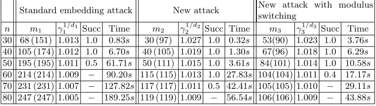
Table 3: Results of the embedding technique using BKZ for binary-LWE using the standard approach and the new lattice rescaling (with and without modulus switching). The columnsmiare the number of LWE samples used for the experiments (the value
in parenthesis is the theoretical value for mi from equation (3) or equation (6) as
appropriate). The lattice dimensions are d1 = m1 + 1,d2 = m2+n+ 1 and d3 =
m3+n+ 1. The lattice gapγi is estimated as in equation (2) and the corresponding
Hermite factor isδi=γ1i/di. Column Succ is the success probability observed from 10
trials (where−denotes no success at all).
Standard embedding attack New attack New attack with modulus switching
n m1 γ 1/d1
1 Succ Time m2 γ 1/d2
2 Succ Time m3 γ 1/d3
3 Succ Time 30 68 (151) 1.013 1.0 0.83s 30 (97) 1.027 1.0 0.32s 53(90) 1.023 1.0 3.76s
40 105 (174) 1.012 1.0 6.70s 40 (105) 1.019 1.0 1.30s 67(96) 1.018 1.0 6.29s
50 195 (195) 1.011 0.5 61.71s 50 (111) 1.015 1.0 3.61s 84(101) 1.014 1.0 10.58s
60 214 (214) 1.009 − 90.20s 115 (115) 1.013 1.0 27.83s 104(104) 1.011 0.4 17.17s
70 231 (231) 1.007 − 127.82s 117 (117) 1.011 0.5 42.41s 105(105) 1.010 − 29.11s
80 247 (247) 1.005 − 189.25s 119 (119) 1.009 − 56.54s 106(106) 1.009 − 43.88s
7.2 Modulus switching
We also experimented with modulus switching for the new algorithm. We confirm our theoretical analysis that the performance is worse. As mentioned in Section 5, the best choice for modulus switching is to use q0 such that q0/q ≈ 1/8. The third block in Table 3 records the running time and success probability of the new attack based on modulus switching. Note that we useq0 = 512. The table shows that the success probability is worse than the new attack without modulus switching.
7.3 Enumeration
When solving CVP for practical parameters the state of the art method [15, 16] is to use BKZ pre-processing of the lattice basis followed by pruned enumeration. This is organised so that the time spent on pre-processing and enumeration is roughly equal. We consider these algorithms here. Note that one can expect a similar speedup from our lattice rescaling for the binary-LWE problem, since the volume of the lattice is increased, which creates an easier CVP instance.
We give predictions of the running time for larger parameters using Chen, Liu and Nguyen’s methods [10, 16]: we first preprocess the CVP basis by BKZ-β for some largeβ and then enumerate on the reduced basis.
Writeδ(β) for the Hermite factor achieved by BKZ with blocks of size β. Given a targetδ(β) and dimensionm, Chen and Nguyen [10] described an algo-rithm to estimate the BKZ time. It is observed that a small number of calls to the enumeration routine (for each block reduction in the BKZ-β) is often sufficient to achieve the targetedδ. It boils down to estimating the enumeration time (either for the local basis within BKZ or the full enumeration later), which depends on the number of nodes visited in the enumeration. We use the approach of [10, 16] to estimate the enumeration time, which assumes the Gaussian heuristic and the Geometric Series Assumption (GSA) [25]. Following this approach, and under those assumptions, we estimate the running time for solving binary-LWE with n= 128, q= 4093 in Table 4.
8
Conclusion
We have described a lattice rescaling approach to the binary-LWE problem, and we have given theoretical and experimental results that confirm its superiority to the standard approach. These results are most interesting when the standard deviation of the error distribution is large.
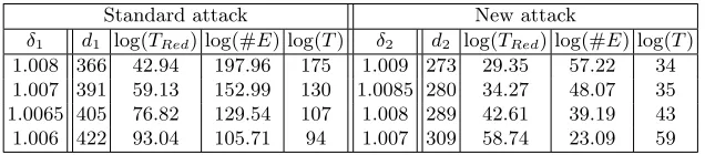
Table 4: Predictions of the running time for solving binary-LWE with (n, q, σ) = (128,4093,22.6) using BKZ lattice reduction followed by pruned enumeration. Columns
diare the lattice dimensions. The BKZ reduction (preprocessing) achieves the targeted
Hermite factorδi. ColumnTRedis an estimate of the BKZ reduction time (in seconds).
Column #E denotes the estimated number of nodes in the enumeration. Column T
denotes the estimated total running-time in seconds.
Standard attack New attack
δ1 d1 log(TRed) log(#E) log(T) δ2 d2 log(TRed) log(#E) log(T)
1.008 366 42.94 197.96 175 1.009 273 29.35 57.22 34 1.007 391 59.13 152.99 130 1.0085 280 34.27 48.07 35 1.0065 405 76.82 129.54 107 1.008 289 42.61 39.19 43 1.006 422 93.04 105.71 94 1.007 309 58.74 23.09 59
Acknowledgements
The authors are grateful to Chris Peikert for suggesting the lattice re-scaling idea. The authors would also like to thank Robert Fitzpatrick, Mingjie Liu, Phong Q. Nguyen and the Program Chairs for helpful comments and discussions.
The authors wish to acknowledge NeSI (New Zealand eScience Infrastructure) and the Centre for eResearch at the University of Auckland for providing CPU hours and support.
References
1. Martin R. Albrecht, Carlos Cid, Jean-Charles Faug`ere, Robert Fitzpatrick and Ludovic Perret, On the Complexity of the BKW Algorithm on LWE, Designs, Codes and Cryptography, Volume 74, Issue 2 (2015) 325-354.
2. Martin R. Albrecht, Robert Fitzpatrick, and Florian G¨opfert, On the Efficacy of Solving LWE by Reduction to Unique-SVP, in Hyang-Sook Lee and Dong-Guk Han (eds), Proceedings of the International Conference on Information Security and Cryptology ICISC 2013, Springer LNCS 8565 (2014) 293-310.
3. Benny Applebaum and David Cash and Chris Peikert and Amit Sahai, Fast Crypto-graphic Primitives and Circular-Secure Encryption Based on Hard Learning Prob-lems, in S. Halevi (ed.), CRYPTO 2009, Springer LNCS 5677 (2009) 595–618. 4. Sanjeev Arora and Rong Ge, New Algorithms for Learning in Presence of Errors,
in L. Aceto, M. Henzinger and J. Sgall (eds), ICALP, Springer LNCS 6755 (2011) 403–415.
5. Anja Becker, Jean-S´ebastien Coron and Antoine Joux, Improved Generic Algo-rithms for Hard Knapsacks, in K. G. Paterson (ed.), EUROCRYPT 2011, Springer LNCS 6632 (2011) 364–385.
6. Avrim Blum, Adam Kalai and Hal Wasserman, Noise-tolerant learning, the parity problem, and the statistical query model, Journal of ACM,50, no. 4 (2003) 506– 519.
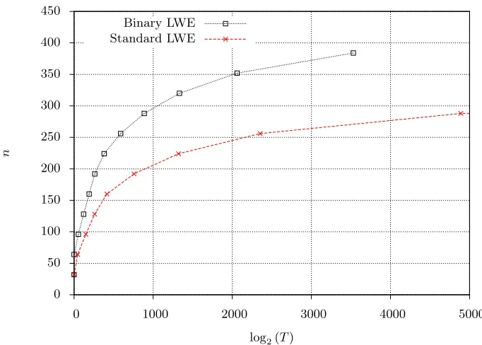
0 50 100 150 200 250 300 350 400 450
0 1000 2000 3000 4000 5000
n
log2(T) Binary LWE
Standard LWE
Fig. 2: Plot of predicted running time with respect to LWE parameternfor embedding attack on standard LWE and binary LWE.
8. Zvika Brakerski, Adeline Langlois, Chris Peikert, Oded Regev and Damien Stehl´e, Classical hardness of learning with errors, in D. Boneh, T. Roughgarden and J. Feigenbaum (eds.), STOC 2013, ACM (2013) 575–584.
9. David Cad´e, Xavier Pujol and Damien Stehl´e, FPLLL, http://perso.ens-lyon.fr/damien.stehle/fplll, 2013.
10. Yuanmi Chen and Phong Q. Nguyen, BKZ 2.0: Better Lattice Security Estimates, in D. H. Lee and X. Wang (eds.), ASIACRYPT 2011, Springer LNCS 7073 (2011) 1–20.
11. Nicolas Gama and Phong Q. Nguyen, Predicting Lattice Reduction, in N. P. Smart (ed.), EUROCRYPT 2008, Springer LNCS 4965 (2008) 31–51.
12. Nicolas Gama, Phong Q. Nguyen and Oded Regev, Lattice enumeration using extreme pruning, in H. Gilbert (ed.), EUROCRYPT 2010, Springer LNCS 6110 (2010) 257–278.
13. Nick Howgrave-Graham and Antoine Joux, New Generic Algorithms for Hard Knapsacks, in H. Gilbert (ed.), EUROCRYPT 2010, Springer LNCS 6110 (2010) 235–256.
14. Ravi Kannan, Minkowski’s convex body theorem and integer programming, Math-ematics of Operations Research12, no. 3 (1987) 415–440.
15. Richard Lindner and Chris Peikert, Better key sizes (and attacks) for LWE-based encryption, in A. Kiayias (ed.), CT-RSA’11, Springer LNCS 6558 (2011) 319–339. 16. Mingjie Liu and Phong Q. Nguyen, Solving BDD by Enumeration: An Update, in
17. Vadim Lyubashevsky and Daniele Micciancio, On Bounded Distance Decoding, Unique Shortest Vectors, and the Minimum Distance Problem, in S. Halevi (ed.), CRYPTO 2009, Springer LNCS 5677 (2009) 577–594.
18. Vadim Lyubashevsky, Lattice signatures without trapdoors, in D. Pointcheval and T. Johansson (eds.), EUROCRYPT 2012, Springer LNCS 7237 (2012) 738–755. 19. Laura Luzzi, Damien Stehl´e and Cong Ling, Decoding by Embedding: Correct
Decoding Radius and DMT Optimality, IEEE Transactions on Information Theory, 59(5), (2013) 2960–2973.
20. Daniele Micciancio and Petros Mol, Pseudorandom Knapsacks and the Sample Complexity of LWE Search-to-Decision Reductions, in P. Rogaway (ed.), CRYPTO 2011, Springer LNCS 6841 (2011), 465–484.
21. Daniele Micciancio and Chris Peikert, Hardness of SIS and LWE with Small Pa-rameters, in R. Canetti and J. A. Garay (eds.), CRYPTO 2013, Springer LNCS 8042 (2013) 21–39.
22. Daniele Micciancio and Oded Regev, Lattice-based cryptography, in D. J. Bern-stein, J. Buchmann, and E. Dahmen (eds.), Post Quantum Cryptography, Springer (2009) 147–191.
23. Oded Regev, On lattices, learning with errors, random linear codes, and cryptog-raphy, in H. N. Gabow and R. Fagin (eds.), STOC 2005, ACM (2005) 84–93. 24. Oded Regev, On lattices, learning with errors, random linear codes, and
cryptog-raphy, Journal of the ACM 56(6), article 34, 2009.