Social Interaction and Self-Organizing Map
Arijit Jha
EdgeVerve Systems Limited 44, Hosur Main Road, Electronics City
Bangalore 560100, Karnataka, India
Abstract– Self Organizing Maps or SOMs are mostly used to represent a multidimensional data in much lower dimension e.g. usually in one or two dimensions, Clustering, Exploratory data analysis and visualization, Supervised data classification, Sampling, Feature extraction, Data interpolation etc. In this paper we consider neuron societies where there are many different types of interactions. In one society, a neuron is connected with others only by the distance between two neurons. In another one, a neuron is connected with others by similarity between neurons, and so on. We here choose a special case where the interaction between neurons is weighted by the distance between them. This simplification aims to apply the new method to the creation of self-organizing maps. With this research, we expect new types of self-organizing maps to appear, ones which take into account the interactions between neurons. Here I have taken data of an automobile industry in Japan over a span of years and analyzed those data.
Keywords– Self Organizing Map, SOM, Artificial Neural Network, Neurons, Society of neurons, Social Interaction, PCA
I. INTRODUCTION
The self-organizing map (SOM) [1] is one of the most well-known techniques in neural networks. In particular, the SOM is commonly used for the visualization of complex data. Contradictorily, one of the main problems of the SOM is that it is difficult to represent final SOM knowledge. This is because self-organizing maps are generally only concerned with competition and cooperation between neurons, without due attention being paid to visualization in the course of learning. Thus, there have been many attempts to visually represent SOM knowledge [1], [2], [3], [4], [5], [6], [7], [8], [9]. However, it is still presently difficult to visualize SOM knowledge clearly; thus, the present study is an additional attempt at clearly visualizing SOM knowledge.
The hypothetical improved visualization is possible by enhancing the characteristics common to neurons based upon their interactions. In addition, our method can be used to control the degree of interaction or cooperation, which contributes to the better visualization of SOM knowledge. Similar method is applied to the analysis of Japanese automobile production for a period of twenty years. The automobile industry underwent drastic changes during these years due to severe competition in the development of environmentally friendly and fuel-efficient cars, and in reducing production costs. However, because of the lack of the methods to clarify the overall characteristics of the automobile industry, it has been difficult to clarify the main characteristics of automobile production. This method is expected to focus upon the important characteristics of the automobile industry through social interaction, because two
neurons with similar outputs interact with each other. Even if the conventional SOM does not create interpretable representations, our method can be used to create interpretable representations by controlling the degree of interaction.
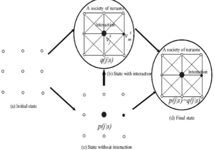
Fig. 1 Social Interaction from an initial state (a) to a final state (d)
In Section II, given the explanation of a concept of social interaction and how to compute social interaction. Then, the method is applied to the self-organizing maps. Here I define the KL-divergence between neurons in interaction and usual neurons. By minimizing the KL-divergence, I derive the optimal outputs and connection weights. In Section III, the experimental results applied to the extraction of characteristics of automobile production from the period of 1993 to 2011 in Japan are presented. I will first determine the optimal representation to maximize mutual information between neurons and input patterns. Then, I will try to interpret connection weights. In the discussion section, I will try to interpret the final representations based on the events and incidents of this period.
II. THEORY AND COMPUTATIONAL METHODS A. Social Interaction
Here we consider societies formed by the interaction of neurons. Suppose that two neurons’ outputs are represented by vj and vm, respectively as shown in
Figure 1. Then, the interaction is defined by the product of two neurons’ outputs:
interactjm = vjvm (1)
In addition, the distance between two neurons should be considered. Now, suppose that the distance is represented by hjm. Then, the interaction is modified as
interactjm = vjhjmvm (2)
m=M
interactj = ∑vjhjmvm (3) m=1
The relative output after the interaction becomes m=M
q(j) = (interactj)/∑interactm (4) m=1
Then, let us suppose that neurons gradually transform from an initial state of society without interaction in Figure 1(a) to a final state with interaction in Figure 1(d). Thus, I should develop a method to model this transformation. Now, let p(j) denote the relative output without the interaction of the jth neuron. Then, this neuron must imitate
the corresponding neuron with interaction. The difference between two types of neurons can be defined by the KL-divergence:
M
D = ∑p(j)log p(j)/q(j) (5) j=1
A society of neurons is formed by minimizing this KL-divergence. By minimizing this divergence, the relative output p(j) becomes closer to the output after the interaction.
B. Application to SOM
Let us apply the concept of a society of neurons to the self-organizing maps. The sth input pattern of total S
patterns can be represented by xs = [x
1s,x2s,…,xLs]T where s
= 1,2,..,S. Connection weights into the jth neuron of total M neurons are computed by wj = [wj1,wj2,…,wjL]T, j =
1,2,…,M. Then the jth neuron’s output can be computed by vjsα exp{-½ (xs-wj)T ˄ (xs-wj)} (6)
where xs and wj are supposed to represent L-dimensional input and weight column vectors, where L denotes the number of input units. The L X L matrix ˄ is called a “scaling matrix”, and the klth element of the matrix is
denoted by (˄)kl is defined by
(˄)kl = δkl k,l= 1,2,….,L (7)
where σα is a spread parameter and is defined by
σα= (8)
Now let us consider the neighbourhood function generally used in self organizing maps
hjcα exp( -
‖
) (9)
where rj and rc denote the position of the jth and the cth unit
on the output space and σγ is a spread parameter. Using this neighborhood function, we have
(
)
(
)
exp
21 1 j s T j s M mjm
x
w
x
w
h
(10)
The relative output of the jth neuron with interaction can be obtained by
q(j|s) = (interactjs)/(∑ ) (11)
Let p(j|s) denote the relative output from the jth neuron
without interaction; then KL divergence is defined by
D = ∑ ∑ p s p j|s log || (12)
By minimizing this divergence we have,
p*(j|s) =
|
21(
x
s
w
j)
T
(
x
s
w
j)
∑ |
21(
x
s
w
m)
T
(
x
s
w
m)
(13)Then by substituting p(j|s) for p*(j|s) we have the well known well known free energy function [10], [11]
F =
2 ∑ p s log ∑ q j|s exp
21(
)
(
)
j s T j s
w
x
w
x
(14)
By differentiating the free energy, we can have connection weights
wj =
∑ ∗ |
∑ ∗ | (15)
III. EXPERIMENTS A. Data Description and Network Architecture
The automobile industry has undergone drastic changes these days because of the increasing interest in environmental problems and severe competition between different automobile manufacturers around the world. In particular, the Japanese automobile industry has undergone major changes in developing advanced technologies and lowering the costs of manufacturing. In advanced technologies, much focus has been upon more fuel-efficiency automobiles, like electric, hybrid, and fuel cell vehicles. In addition, the high appreciation of the Japanese yen has made it impossible to produce automobiles with lower costs in Japan. Thus, it is certain that these drastic changes have been observed in the production and sales of automobiles in Japan. However, it has been difficult to extract the overall characteristics from complex automobile production and sales data. I here focus upon the analysis of automobile production and try to show the main characteristics of the production over these twenty years.
Fig. 2 Network architecture for the automobile data
Fig. 3 Mutual information as a function of the parameter α(a) and with a fixed value (1/10) of the parameter α(b)
B. Optimal representation and mutual information
The social interaction method can produce many different types of networks by taking into account the degree of interaction and competition. The degree of interaction can be changed through the parameter α. Thus, we must choose an appropriate representation among them. One of the possibilities is to use mutual information between neurons and input patterns. When this mutual information is
increased, neurons tend to contain more information on input patterns. Mutual information can be defined by
I(α) = ∑ p s ∑ p s p j|s; α log | ;; (16) One of the problems with this mutual information is that it increases constantly when the Gaussian width decreases or the parameter αincreases, as shown in Figure 3(a). Thus, we must assign a constant value to the parameter α. Note that in actual learning, the parameter α was changed from one to ten, and the parameter was fixed only for computing mutual information. Figure 3(b) shows this mutual information when the parameter α was set to 1/10. As can be seen in the figure, mutual information increased initially and reached its highest point when the parameter αwas 4. Then, mutual information gradually decreased. Though mutual information increased when the parameter α was increased in Figure 3(a), the actual mutual information did not increase when the parameter αwas increased from 4 in Figure 3(b). Thus, we can say that when the parameter α was 4, we could obtain an optimal representation which had the maximum amount of information on input patterns.
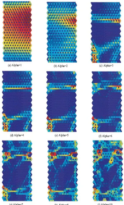
Fig. 4 U matrices when the parameter α was changed from 1(a) to10(i)
clearer, and other class boundaries began to appear on the lower side of the matrix. When the parameter α was 4 in Figure 4(d), the class boundary on the upper side of the matrix became the clearest and the other boundaries on the lower side became much clearer. Then, when the parameter α was further increased from 5 in Figure 4(e) to 10 in Figure 4(i), the class boundaries began to gradually deteriorate. These results corresponded to those of mutual information in Figure 3(b). When mutual information was 4, we could obtain maximum information, and then mutual information gradually decreased. When mutual information reached its maximum, the clearest representation in Figure 4(d) could be obtained.
Fig. 5 U matrices (1) and labels(2) when the parameter α was 4
C. Interpretation of optimal representation
I interpret the optimal representation with maximum mutual information when the parameter αwas 4. Figure 5 shows the U-matrix and labels with class boundaries when the parameter α was 4. As shown in Figure 5(1), a clear class boundary in warmer color could be detected on the upper side of the matrix. Additionally, several minor class boundaries were located on the lower side of the matrix. From these boundaries and labels in Figure 5(2), the data was classified into three classes (periods). The first period (a) represented the production from 1993-1998. The second period ranged between 1999 and 2006, and the third period between 2007 and 2011. In the third period, the period between 2007 and 2008 and the year 2011 were separated from the period in the middle. In addition, we can see that in the first and the third periods, the data were arranged from right to left. On the other hand, in the second period, the data were arranged from left to right.
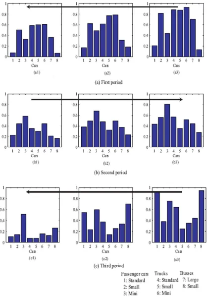
Fig. 6 Connection weights from all variables when the parameter α was 4
Figure 6 shows connection weights from the eight variables. As shown in Figure 6(a3), in the second and third periods, the production of mini-cars was very large, shown in warmer colors. On the other hand, standard, small and mini trucks were more heavily produced in the first period, in Figure 6 (b1), (b2) and (b3). In the third period, standard passenger cars and small buses were produced largely, represented by warmer colors in Figure 6(a1) and (c2). In addition, for all variables, the parts on the left hand at the bottom were very low in dark blue. This means that the production of automobiles was the lowest around 2011.
production of standard passenger cars and small buses were much higher than that of any other type of cars. However, the production decreased gradually in Figure 7(c2). Finally,
in 2011, shown in Figure 7(c1), though overall production was very low, the production of mini-cars remained relatively higher.
Fig.8 Umatrix (a) and labels (b) by the conventional SOM
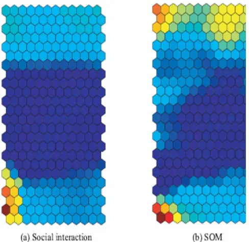
Fig. 9 Information content of neurons by social interaction (a) and by SOM (b)
D. Comparison of SOM wth PCA
We here compare the results of our method with those obtained by the standard SOM and PCA. Figure 8 shows the U-matrix and labels by the conventional SOM. We used the SOM toolbox for the experiments [4]. As can be seen in Figure 8(a), two class boundaries in warmer colors appeared on the upper side and the lower left hand side of the matrix, but they were rather ambiguous. Labels in Figure 8(b) show that the class boundaries in Figure 8(b) corresponded to those in Figure 5(2).
Figure 9 shows information contained in the jth
neuron on the input neurons. Let p(k|j) denote the relative output of the kth input neuron for the jth neuron; then,
information for the jth neuron on the input neurons is
defined by
Ij = log L + ∑ p k|j log | (17)
where
p(k|j) = ∑ (18)
Figure 9 shows this information computed by the social interaction (a) and SOM (b). As shown in Figure 9(a), we could see three classes on the map by the social interaction. On the other hand, by the SOM, as in Figure 9(b), boundaries between three classes were not always clear. On the lower left hand side of the maps by the social interaction and SOM, neurons with the highest information on input neurons appeared. This part corresponded to year 2011, where only mini-car was produced largely. This proves that the year 2011 showed the most explicit characteristic of all periods. Namely, the number of mini cars was much larger than any other cars in terms of production.
Figure 10 shows the results of PCA applied to data itself (a), connection weights by the conventional SOM (b) and social interaction (c). With the PCA applied to the data itself, seen in Figure 10(a), three classes were observed but they were extensively overlapping. Figure 10(b) shows the results of PCA applied to the connection weights by the conventional SOM. Though three classes could be observed, many weights were scattered between boundaries. Finally, when the social interaction was used in Figure 10(c), the classes were clearly separated
E. Discussion
1) Summary of Results: Let us summarize the main results of the automobile production. In 2000s, the automobile production gradually decreased as shown in Figure 7(a3) to (a1). In the second period (the beginning of 1990s), the production inversely increased, and in particular, the production of mini-cars increased as shown in Figure 7(b3) to (b1). Then, in the beginning of the third period (2007 and 2008), the production of standard passenger cars and small buses increased significantly, shown in Figure 7(c3). The production then decreased again in Figure 7(c2). Finally, in 2011, only the production of mini-cars maintained relatively high production rates, while all the other types of car showed rather low production rates, as shown in Figure 7(c1).
2) Explaining by Actual Events: These characteristics can be explained by the two important factors occuring in these periods: the revised regulation law for mini cars and the economic crisis called the "Lehman shock."
First, the class boundary between the first and second period could be explained by the revised regulation law for mini cars in 1998. In the first period, all types of cars were being produced equally, except standard and mini-cars and small buses. In the 2000s, only the production of mini-cars increased, albeit gradually. We examined the events and incidents around this boundary period, and found that the automobile regulation by the Japanese government was revised in 1998. In the revision of the safety regulation for the mini-cars in 1998, the size of mini-cars became larger and the safety levels became higher, obtaining performance comparable to that of larger cars. Because of this revision of the regulation, the Japanese automobile market was drastically changed around 1998.
Second, the third period was explained by the economic crisis of 2008. We could observe the high production in standard passenger cars and small buses in the beginning of the third period in Figure 7(c3) around 2007 and 2008. In this period, we recognized the well-known "Lehman Shock" phenomenon following the economic crisis, which damaged the Japanese automobile industry. In particular, the increase in the production of standard passenger cars in this period was one of the main causes of troubles in the automobile industry.
3) Implication for Automobile Industry: Considering these results and facts, we can point out two factors concerning the automobile industry, namely, policy and planning.
First, one important factor in the development of automobile industry is the policy for the industry. It is necessary to guide the industry through the effective and industrial policy, conceptualized and implemented by the government. In our experimental results, the revised regulation law for the mini-cars drastically changed the market, leading to a sharp increase in the production of mini cars.
Second, production should be more carefully planned. The increase in production in the beginning of 2000s had long lasting negative effects on the automobile industry. We observed that the production in the beginning of 2000s was focused on mini cars, meaning that smaller cars were generally preferred. Despite this, standard passenger cars were largely produced in the beginning of the period. Even if the majority were for export purposes, more restrained production should have been expected, which would have led to lessened damages from the economic crisis.
4) Problems of the Method: Though our method has shown better performance in visualization, we should point out two problems, namely, optimality and topological preservation.
First, we used mutual information to obtain optimal representations. In other words, mutual information was used to choose the optimal values of the parameter a. When mutual information increases, neurons tend to respond very specifically to input patterns. By increasing mutual information, representations become simpler. However, one of the problems is that we did not increase this mutual information, but rather decreased KL-divergence. Thus, we need to examine the relation between KL-divergence and mutual information more carefully.
Second, we should examine the relations between visualization and topological preservation. We have shown that the method worked better to clarify class boundaries. When visualization can be improved, it may happen that topological relations cannot be maintained. This is because better visualization enhances some parts of input patterns, reducing topological preservation. However, we have not yet finished examining the relations between the improved performance and topological preservation. Even if the performance in visualization is improved, if topological relations are not preserved, then the reliability of the final maps decreases. Thus, we should more precisely examine the relationship between visual performance and topological preservation.
5) Possibilities of the Method: The main possibilities of the method are summarized by two points, namely, flexibility and new self-organizing maps.
present probabilities q(j | s) by new ones. For example, we can imagine a case where even if the distance between neurons is very large, they still may strongly be connected with each other. We can take into account this kind of interaction.
Second, we can create new types of self-organizing maps based upon the social interaction. As mentioned above, our method can create a variety of interactions between neurons. Based upon these different types of interaction, it is possible for networks to self-organize, leading to characteristics different from those by the conventional SOM. If we take into account the different types of cooperation between neurons, new types of self-organizing maps can be created.
IV. CONCLUSION
In this chapter, we proposed a new type of information-theoretic method in which neurons are supposed to form a society. In this society, the interaction of neurons is the product of all neighboring neurons’ outputs weighted by their distance. The individual neuron tries to imitate this interaction as much as possible. The difference between neurons with and without interaction is computed by the KL-divergence. By minimizing the KL-divergence, we can obtain the optimal outputs of the neuron and the free energy. By differentiating the free energy, we can obtain the re-estimation rules for connection weights.
We applied our method to the data of the production of Japanese automobiles during the period of 1993 and 2011. We can summarize the final results from two points of view. Technically, the new method showed better performance in clarifying class boundaries, compared with the conventional SOM. Explicit class boundaries were due to the interaction of neurons, similar neurons interacting strongly with each other in terms of distance and firing rates. Second, the strong class boundaries were traced back to the important events or incidents which occurred in the period. For example, the class boundary between the first and the second period was due to the revision of regulation law for mini-cars. Thanks to this revision, the number of mini-cars in production increased gradually. In the third period, a significant production increase at the beginning of the period was accompanied by a decrease in production of other models, with only mini-cars being largely produced in the end. This period was well explained by the economic crisis in 2008.
Though there are some problems such as optimality and topological preservation, as explained in the discussion section, we have shown that it is possible to create different types of neuron societies, where different kinds of interaction can be implemented.
ACKNOWLEDGEMENT
I would like to thank a few people without whom this could not be completed. First and foremost I would like to show my gratitude towards Mr.Sourav Dutta, faculty of Department of Computer Science, Netaji Subhash Engineering College, West Bengal University of Technology, for his continuous support by providing the necessary information and educating me about the topic. Then I would like to mention about Mr. Anil Jalagam, Product Manager of AssistEdge, EdgeVerve Systems Ltd. for enriching me with all his knowledge in the concerned field. And at last thanks to all my collegues for their continuous support and help during data collection and analysis phase. Without all you people this wouldn’t have seen the light.
REFERENCES
[1] Kohonen, Teuvo (1982). "Self-Organized Formation of Topologically Correct Feature Maps". Biological Cybernetics43 (1):
59–69.
[2] Ultsch, Alfred; Siemon, H. Peter (1990). "Kohonen's Self Organizing Feature Maps for Exploratory Data Analysis". In Widrow, Bernard; Angeniol, Bernard. Proceedings of the International Neural Network Conference (INNC-90), Paris, France, July 9–13, 19901. Dordrecht,
Netherlands: Kluwer. pp. 305–308. ISBN 978-0-7923-0831-7. URL:
http://www.uni-marburg.de/fb12/datenbionik/pdf/pubs/1990/UltschSiemon90
[3] J.W. Sammon. A nonlinear mapping for data structure analysis. IEEE Transactions on Computers, C-18(5):401–409, 1969.
[4] A. Ultsch and H. P. Siemon. Kohonen self-organization feature maps for exploratory data analysis. In Proceedings of International Neural Network Conference, pages 305–308, Dordrecht, 1990. Kulwer Academic Publisher.
[5] A. Ultsch. U*-matrix: a tool to visualize clusters in high dimensional data. Technical Report 36, Department of Computer Science, University of Marburg, 2003.
[6] R. Kamimura. Self-enhancement learning: target-creating learning and its application to self-organizing maps. Biological cybernetics, pages 1–34, 2011.
[7] R. Kamimura. Constrained information maximization by free energy minimization. International Journal of General Systems, 40(7):701– 725, 2011.
[8] Hujun Yin. ViSOM-a novel method for multivariate data projection and structure visualization. IEEE Transactions on Neural Networks, 13(1):237–243, 2002.
[9] Lu Xu, Yang Xu, and Tommy W.S. Chow. PolSOM-a new method for multidimensional data visualization. Pattern Recognition, 43:1668–1675, 2010.