Improved Apriori Algorithm – A Comparative study using different Objective measures

(1)

Improved Apriori Algorithm – A Comparative

study using different Objective measures.

Prof. Dr. K. Rajeswari HOD, Dept. of Computer Engineering Pimpri Chinchwad college Of Engineering Pune, India

Abstract – Apriori algorithm is a popular and classical algorithm in data mining. The apriori algorithm has certain disadvantages too. This paper discusses about 6 improved apriori algorithms, new techniques used, how they are more efficient as compared to traditional apriori algorithm. Paper also provides comparisons of algorithm based on certain important attributes, identifies the strength and weakness and proposes future work in this domain. Different objective measures to identify relationship between attributes are also discussed.

Keywords – Data mining, Apriori algorithm, Improved Apriori, Objective measures.

1. INTRODUCTION

There is a huge amount of data around us and to extract valuable information data mining is used. Data mining is defined as the process of discovering interesting patterns in data. Data mining is about solving problems by analyzing the data present in the database and identifying useful patterns. Patterns allow us to make prediction on new database. Association rule mining techniques is an important concept in data mining which is used to describe association between various item set among large amount of data. Many algorithms come under association rule mining but Apriori algorithm is one of the typical algorithms. It was introduced by Agarwal in 1993; it is a strong algorithm which helps in finding association between itemsets. A basic property of apriori algorithm is “every subset of a frequent item sets is still frequent item set, and every superset of a non-frequent item set is not a frequent item set”[1]. This property is used in apriori algorithm to discover all the frequent item sets. Further in the paper we will discuss more about the different objective measures used for finding relationship between variables, properties of objective measures, Apriori algorithm steps in detail and Improved Apriori algorithms.

1.1 Traditional Apriori Algorithm

Before going into details of Apriori algorithm we will first see the definitions of some common terminologies which are used in algorithm [8].

Itemset - Itemset is collection of items in a database which is denoted by I = {i1, i2,…, in}, where n is the number of

items.

Transaction – Transaction is a database entry which contains collection of items. Transaction is denoted by T and T  I. A transaction contains set of items T={i1,i2,..,in}.

Minimum support – Minimum support is the condition which should be satisfied by the given items so that further processing of that item can be done. Minimum support can be considered as a condition which helps in removal of the

in-frequent items in any database. Usually the Minimum support is given in terms of percentage.

Frequent itemset – The itemsets which satisfies the minimum support criteria are known as frequent itemsets. It is usually denoted by Liwhere i indicate the i-itemset.

Candidate itemset – Candidate itemset are items which are only to be consider for the processing. Candidate itemset are all the possible combination of itemset. It is usually denoted by Ciwhere i indicate the i-itemset.

Support – Usefulness of a rule can be measured with the help of support threshold. Support helps us to measure how many transactions have such itemsets that match both sides of the implication in the association rule.

Consider two items are there A and B to calculate support of A  B the following formula is used,

Support(AB)

= (number of transaction containing both A & B) (Total number of transaction)

Confidence –Confidence indicates the certainty of the rule. This parameter lets us to count how often a transaction’s itemset matches with the left side of the implication in the association rule also matches for the right side. The itemset which does not satisfies the above condition can be discarded.

Consider two items are there A and B to calculate confidence of A  B the following formula is used,

Conf(AB)

=(number of transaction containing both A & B) (Transaction containing only A)

Note:Conf(AB) might not be equal to conf(BA).

Aprioir Algorithm -Apriori algorithm works on two concepts a)Self Join and b)Pruining. Apriori uses a level-wise search where K-itemsets are used to find (K+1 )-itemset.

1. First, the set of frequent 1- itemsets is found which is denoted by C1.

2. The next step is support calculation which means the occurance of the item in the database. This requires to scan the complete database.

3. Then the pruning step is carried out on C1in which the

items are compared with the minimum support parameter.The items which satisfies the minimum support criteria are only taken into consideration for the next process which are denoted by L1.

4. Then the candidate set generation step is carried out in which 2-itemset are generated this is denoted by C2.

(2)

which satisfies the minimum support criteria are further used for 3-itemset candidate set generation. 6. This above step continues till there is no frequent or

candidate set that can be generated.

We can easily understand the concepts used by the aprioir with the help of following example. Table 1 shows a transactional database having 4 transactions. TIDis a unique identification given to the each transaction.

TABLE 1 SAMPLE DATABASE

TID Items

T001 A, C, D T002 B, C, E T003 A, B, C, E

T004 B, E

Performing the first step that is scanning the database to identify the number of occurance for a particular item. After the first step we will get C1 which is shown in Table

2.

TABLE 2 C1

Itemset Support

{A} 2 {B} 3 {C} 3 {D} 1 {E} 3

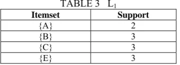
The next step is the pruning step in which the itemset support is compared with the minimum support. The itemset which satisfies the minimum support will only be taken further for processing.Assuminig minimum support here as 2. We will get L1 from this step. Table 3 shows the

result of pruining.

TABLE 3 L1

Itemset Support

{A} 2 {B} 3 {C} 3 {E} 3

Now the candidate generation step is carried out in which all possible but unique 2-itemset candidates are created. This table will be denoted by C2. Table 4 shows all the

possible combination that can be made from Table 3 itemset

TABLE 4 C2

Itemset Support

{A, B} 1

{A, C} 2

{A, E} 1

{B, C} 2

{B, E} 3

{C, E} 2

Now pruning has to be done on the basis of minimum support criteria. From Table 4 two itemsets will be removed. After pruning we get the following results.

TABLE 5 L2

Itemset Support

{A, C} 2

{B, C} 2

{B, E} 3

{C, E} 2

The same procedure gets continued till there are no frequent itemsets or candidate setthat can be generated. The further processing is described in Table 6 and Table 7.

TABLE 6 C3

Itemset Support

{A,B,C} 1 {A,B,E} 1 {B,C,E} 2

TABLE 7 L3 FINAL RESULT

Itemset Support

{A,B,C} 1 {A,B,E} 1 {B,C,E} 2

Pseudo Code -

Ck: Candidate itemset of size k

Lk : frequent itemset of size k

L1 = {frequent items};

for (k = 1; Lk !=; k++) do begin

Ck+1 = candidates generated from Lk; for each transaction t in database do

increment the count of all candidates in Ck+1that are

contained in t

Lk+1 = candidates in Ck+1 with min_support end

returnkLk;

Drawbacks of Apriori algorithm

 Large Number of infrequent itemset are generated which increases the space complexity.

 Too many database scans requires because of large number of itemsets generated.

 As the number of database scans are more the time complexity increases as the database increases.

Due to these drawbacks there is a necessity in making some modification in the Apriori algorithm which we will see further in this paper.

1.2 Improved Apriori Algorithms

1.2.1 Improved apriori based on matrix[2]

Events: One transaction of commodity is an event. That is Event = 1 Transaction containing various Items.

Event Database (D): An event T in D can be shown as Ti<i1,i2,i3,…,in> , Where Ti is unique in the whole Database.

First step in this improved apriori is to make a Matrix library. The matrix library contains a binary representation where 1 indicated item present in transaction and 0 indicated it is absent. Assume that in the event Matrix library of database D, the matrix is A mxn , then the corresponding BOOL data item set of item Ij(1<= j <= n)in P in Matrix Amxn is the mat of Ij, Mati is items in the mat.

(3)

TID LIST OF Items I1 I2 I3 I4 I5

T001 I1, I2 ,I5 1 1 0 0 1 T002 I2, I4 0 1 0 1 0 T003 I2, I3 0 1 1 0 0 T004 I1 ,I2 ,I4 1 1 0 1 0 T005 I1, I3 1 0 1 0 0 T006 I2, I3 0 1 1 0 0 T007 I1, I2 1 1 0 0 0 T008 I1, I2, I3, I5 1 1 1 0 1 T009 I1, I2, I3 1 1 1 0 0

For 1-itemset matrix represented is used (i.e.) MAT(I1) = 100110111

MAT(I2) = 111101111 MAT(I3) = 001011011 MAT(I4) = 010100000 MAT(I5) = 100000010

Now by counting the number of 1’s in the matrix we can easily fint the occurance of that item.

For 2-itemset we can just multiply the binary representation of the items to get the occurance to that items together. To find how many times item Ij and Ik are appearing

together we have to multiply the MAT(Ij) and MAT(Ik).

(i.e) MAT(Ij,Ik)=MAT(Ij) * MAT(Ik).

MAT(I2,I5)=MAT(I2) * MAT(I5) = 100000010 * 111101111 = 100000010

Mat(I2,I5) = 100000010

Then support of these two items can be calculated as follows:

Support (I2, I5) = (Nos. of times Appearing together/Tot. Transaction) = 2 / 9

Similarly the same procedure can be followed for all possible itemset. This algorithm needs to scan the database only once and also does not requires to find the candidate set when searching for frequent itemset.Table 9 provides the computational time of Apriori and improved apriori.

TABLE 9 COMPUTATION TIME FOR APRIORI AND IMPROVED APRIORI

Record number

Apriori Computing time(ms)

Improved Apriori Computing time(ms)

500 1787 35

1000 8187 108

1500 44444 178

2000 46288 214

2500 97467 292

3000 199253 407

3500 226558 467

4000 310379 569

5000 155243 470

1.2.2 Improved apriori using hash structure[3]

The IMPROVED-APRIORI algorithm uses Hash structure which optimizes 2-items generation which improves the save time and space. Using the IMPROVED-APRIORI algorithm directly L2 is generated from only one database scan without generation of C1, L1 and C2. By using hash table instead of hash tree the searching cost is reduced. The L2 is directly generated using an hash function.

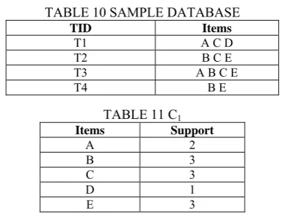
The first step is to read the database once and make a hash table which includes each itemset and its support. Table 10 shows sample database and Table 11 shows the results of first step.

TID Items

T1 A C D

T2 B C E

T3 A B C E

T4 B E

TABLE 11 C1

Items Support

A 2 B 3 C 3 D 1 E 3

Before going to next step we will discard the items which does not satisfies the minimum support criteria. The next step suggested in APRIOIR-IMPROVE is to make combination of 2-itemsets for each transaction (i.e.) if transaction 1 contains items like A B C then possible combination would be {AB} {AC} {BC} so by applying this process we get the following results.

TABLE 12: MAKING COMBINATION

TID Items

T1 {AC} {AD} {CD} T2 {BC} {BE} {CE}

T3 {AB} {AC} {AE} {BC} {BE} {CE} T4 {BE}

Now by using the following Hash function we will store the support of each combination Table 13

Hash Function: H(x,y) = (P(x)-1)*(N-1)+P(y)-P(x)*(P(x)-1)/2-1

TABLE 13 HASH STRUCTURE

AB AC AD AE BC BD BE CD CE DE 1 2 1 1 2 0 3 1 2 0

From the above table we get L2 (i.e.) after pruning the above table data we can get the 2 Item set. Similarly for the further candidate set generation we use the same procedure. Using a different storage structure and different pruning method the number of scan required to form the 2nd_{Item set}

is reduced to one which in far better than traditional apriori algorithm. Hence this will be effective if there is less number of items as for storing and retrieving hash table and hash function will be used. More number of items leads to more number of combinations and more number of combination leads to more number of storage.

1.2.3 Improved Algorithm for Weighted Apriori[4] In traditional apriori meaningless frequent itemset exist that increases the database scans and requires lots of storage space.

(4)

steps like pruning and selection can be done according to the minimum weighted support and confidence.

Let I = (i1,i2,i3,….,ij) is a set of items and T=(t1,t2,….,tn) is the set of transactions.

Weights (wi) are assigned to each Transaction ti, where 0 ≤ wi ≤ 1, (i=1,2,…n). K is K-itemset.

The weighted confidence will be calculated using the following formula:

TABLE 14: SAMPLE DATABASE

TID Product List TID Product List

1 A1,B1,B2,D1 6 A1,A2,D1 2 A2,B1,C1 7 A2,B1,B2 3 A1,A2,B2,D1 8 A1,A2,B2 4 A1,C1,D1 9 B1,B2 5 A1,A2,B1,B2,D1 10 A1,A2,C1,D1

Here we will consider supermarket example where A, B, C, D are considered as categories according to the types of goods. A, B, C, D each has several kinds of merchandise goods.

The next step will be setting the weights according to the categories. The weight values indicate the degree of importance of the interrelation of the goods.

Now using the Traditional apriori two methods (i.e.) Pruning and connecting

First step: Connect; this will connect the frequent item with candidate set.

TABLE 15: SUPPORT CALCULATION

Item set Supporting degree count

Supporting degree

Weighted supporting

degree

A1 7 70% 70% A2 7 70% 70% B1 4 40% 36% B2 5 50% 45% C1 3 30% 24% D1 6 60% 42%

Second step: Pruning; this step will scan the database and remove the items which do not satisfies the minimum support criteria. So by considering minimum support as 30% for above database we get the following results.

TABLE 16: DATABASE AFTER PRUNING

Supporting degree

degree

A1 7 70% 70% A2 7 70% 70% B1 4 40% 36% B2 5 50% 45% D1 6 60% 42%

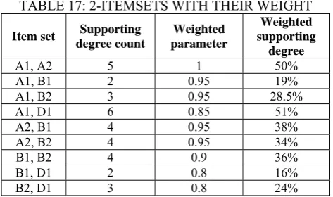
The next step includes creation of 2-Itemset so all possible combination are made. For above database following combinations are possible.

TABLE 17: 2-ITEMSETS WITH THEIR WEIGHT

Weighted parameter

degree

A1, A2 5 1 50%

A1, B1 2 0.95 19% A1, B2 3 0.95 28.5% A1, D1 6 0.85 51% A2, B1 4 0.95 38% A2, B2 4 0.95 34%

B1, B2 4 0.9 36%

B1, D1 2 0.8 16%

B2, D1 3 0.8 24%

Again the pruning step is carried out which scans the database and removes the items which do not satisfies the minimum support criteria. Then for further itemsets generation the apriori method is followed.

In this paper the same procedure is carried out as in Apriori but the only difference is that instead of taking all the items we will make a group and then apply the apriori algorithm on it. Due to which the scans are faster, less number of space is required as compared to traditional algorithm. But making groups requires a lot of analysis; if no analysis is made improper groups can create an invalid association of items

1.2.4 Improved apriori - OOO algorithm[5]

This paper proposes a new strategy of accessing the database which significantly improves the performance of the Apriori algorithm. Not only computation efficiency is improved the time and space complexity is also improved. The OOO algorithm proposed in this paper need only one database scan. The steps carried out in this algorithm are - initially the database is scanned and support degree of each item is calculated. This algorithm will not produce the candidate item whose support degree is 0 which will reduce the number of candidate items. The 10 details OOO algorithm processes are as follows:

Step 1: Read DB, set i=1, candidate set C=Φ, frequent set L=Φ

Step 2: if i>|DB|, go to Step 10 Step 3: set t=Ri, compute j=|t|

Step 4: if j=0, go to Step 9

Step 5: Cj={x|x⊆t∧|x|=j}. If x∈Cj∧x∈L, Cj=Cj–x Step 6: C=CU Cj∧x. count=x. count+1

Step 7: if x∈C∧x. count=min_sup, L=L {y|y ⊆x }∧C=C–x Step 8: j=j-1, go to Step 4

Step 9: i=i+1, go to Step 2

Step 10: Close database and start producing association rule Time Complexity of OOO algorithm

f’(k)=|DB|+(|R1|+|R2|+…+|Rj|)∑ki=1 (|Ci|+|Li|)

Where DB is database, Ri is record i.

Table 18 Indicates the execution process of OOO Algorithm. Suppose sample data is there and there are four records: ABC, BCD, ABCE, BD. Table 18 shows the complete execution of OOO algorithm.

∑

Wi

(Ti ε(xUY)/K)(S(x  y)) ≥ w min i sup

∑

Wi

(5)

The first transaction is scanned and the 1-itemset column is filled (i.e.) C1 column. If the items are repeated in the next transaction then the count of the item is incremented. After the complete scanning of the database we get L1 column which is then used for 2-itemset candidate set generation. C2 column is filled with possible combination of two items and simultaneously count is also incremented if the same items are repeated in the next transaction.

TABLE 18 COMPLETE EXECUTION OF OOO ALGORITHM

ITE MS

C4/C ount

C3/C ount

C2/C ount

C1/C ount

L3/C ount

L2/C ount

L1/C ount

ABC ABC AB A

AC B

BC C

BCD BCD BC/2 D BC/2 B/2

BD C/2

CD

ABC E

ABC/

2 AE E

ABC/

2 AB/2 A/2

ABE BE AC/2 B/3

ACE CE BC/3 C/3

BCE

BD BD/2 ABC/₂ AB/2 A/2

AC/2 B/4

BC/3 C/3

BD/2 D/2

These steps are followed till there are no frequent items to generate from any transaction This algorithm scans the database only once and also does not generate the candidates whose occurrence is 0. By scanning the database only once we can identify the counts of items which are more likely to come together.

1.2.5 Improved algorithm based on Interest itemset[6] The improved apriori algorithm suggested in this paper proposes that by using the interest items the candidates set can be reduced and also the speed of the algorithm is accelerated. This algorithm is based on interest measures. There are some constraints on the selection of interest itemset. These constraints are:

Selection of interest items is done by user. These items are denoted by Itsnand collection of interested itemset are

denoted by Its = {its1, its2,….,itsn}.This algorithm uses

interest items to exclude the items which are not relevant.

TID Items Num L

1 I1, I2 20 2

2 I1, I3, I4 5 3

3 I2, I5, I6 70 3

4 I6, I7 5 3

For example the itemset contains I={I1,I2,I3,I4,I5,I6,I7} and we need to find the association between I1,I2,I3,I4,I5 then the rest are excluded. So Its will contains Its= {I1, I2, I3, I4, I5}.

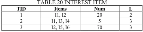
Now the uninterested data is removed from Table 19 and the remaining items will only be present. Table 20 represents the interested items.

TABLE 20 INTEREST ITEM

TID Items Num L

1 I1, I2 20 2

2 I1, I3, I4 5 3

3 I2, I5, I6 70 3

Array structure is used to store data and to reduce the database scans. Following is the array representation of the transaction.

A[]={I1,I2 ; I1,I3,I4 ; I2,I5}

Then the array is traversed to scan the frequent itemset based on the minimum support. The frequent items are inserted into the array {A1, A2, A3, …, An} where n represents length of itemset. So A1 will contain A1[]=={I1,0.25; I2,0.9; I5,0.7} and A2 will contain A2[]={I1,I2,0.2;I2,I5,0.7}.

TABLE 21 COMPARISION OF APRIORI AND IMPROVED APRIORI

Apriori Improved

Apriori

Efficiency improvement

Frequent Itemsets 114 44 61.4% Strong association

rules 51 20 62%

Time 79 24 69.62%

The concept of interested items selection is very efficient in terms of rules generation and database scans. But the drawback could be use of Arrays as array structure has some disadvantages which can become a drawback for the improved apriori algorithm.

1.2.6 Improved Apriori based on transaction compression[7]

The proposed Improved Apriori algorithm works by compressing transaction database, by using an attribute named count the efficiency of the algorithm is improved. The transaction database creates lots of same records after a certain amount of time. For example if we consider the transaction database of super market then applying apriori algorithm on repeated database will require unnecessary scans. So clustering can be done for these kinds of databases. Only one entry is made in the database and whenever the same item in transaction occurs as the previous one it is discarded. To show the frequency of repeated records an attribute is added named count. The next steps are similar to apriori algorithm like candidate set generation and pruning.

(6)

TABLE 22 EMPLOYMENT OF COLLEGE GRADUATE

Seq No. Degree

(Yes/No)

Major

(Hot/Cold) Major score

English Grade

Computer capability

Social Practical

Employment (Yes/No)

1 Yes Hot 85 Level 6 Pass Yes Yes

2 Yes Cold 83 Level 4 Pass Yes Yes

4 No Cold 65 Fail Fail Yes No

6 Yes Cold 86 Level 6 Pass Yes Yes

8 No Hot 87 Fail Pass No No

9 No Cold 71 Level 4 Fail No No

10 No Cold 62 Level 4 Fail Yes No

…… …… …… …… …… …… …… ……

TABLE 23 COLLEGE GRADUATE DATA AFTER PREPROCESSING

Degree (Yes/No)

Major

(Hot/Cold) Major score English Grade Computer capability Social Experience Count

1 1 1 1 1 1 2

1 0 1 1 1 1 2

1 1 0 1 1 1 2

…… …… …… …… …… …… ……

The above student college data is scanned and a new table is created in which the repeated data is placed only once and a new column is added Count which indicate the frequency of the same tuple occurring in the database. With the help of this algorithm huge database can be normalized which reduces the number of transaction. This transaction can then be forwarded to Apriori algorithm and association rules can be found. The database scan frequency is also reduced. The major problem is data preprocessing which will consume a lot of time.

1.2.7 Methods to improve apriori efficiency

•Hash-based itemset counting: Am-itemset whose matching hashing bucket count is lowerthan the threshold cannot be frequent.

•Reduction of Transaction: A transaction that does not contain any frequent m-itemsetis worthless in successive scans.

•Partitioning:Anyitemset that is potentially frequent in Data base must be frequent in at least one of the partitions of Database.

•Sampling:Mining on a subset of given data.

•Dynamic itemset counting:Include new candidate itemsets onlywhen all of their subsets are estimated to be frequent.

2. COMPARISON OF IMPROVED APRIORI

TABLE 24 COMPARISION OF IMPROVED APRIORI

Attributes

Improved algorithm based on

matrix

Improved algorithm based on hash

structure

Improved algorithm based on weighted apriori

OOO algorithm

Improved algorithm based on

Interest Itemset

Improved algorithm based on Transaction compression

New Technique Used

Binary matrix which to reduce

the database scans

Hash structure introduced to quick retrieve data from

database

Large amount of items divided categorized into

groups

New strategy for accessing the database

items

Only the interested items

of user are considered

Pre-processing is done on database to

remove redundancy

Number of scans 1 1 More than 1 1 More than 1 More than 1

Storage structure

used 2-D array Hash Table

Normal Database

Normal

database Array

Normal database

Efficiency improved(against

Apriori)

(7)

3. DISCUSSION

The above comparison clearly states that many new modifications are possible that can improve the efficiency of the apriori. The main attribute that always will be in consideration is the number of database scans. As the number of transaction grows the size of the database increases due to which the number of scans increases. Many algorithms above have suggested a new technique which requires only one database scan. These methods can also further be modified to increase the efficiency of apriori.

Also candidate set generation is another important aspect that should be more focused on. The item sets generation step of apriori many times generatesitem set which are not frequent and most of the time not required. Some algorithms have suggested to scan each transaction and combination of items should be based on items present in the transaction only. But this method will require keeping a track of items which have been traversed, and for doing this again we will require more number of comparison that leads to greater time complexity.

These are some areas which can be focused and which would help in improving the association rule mining’s apriori better and optimized algorithm. In our next paper a new technique will be discussed which will provide a more optimized solution for association rule mining.

4. CONCLUSION

In this paper we have discussed on 6 improved apriori algorithms which provides a new technique in generating rules. These algorithms are more efficient than the traditional algorithm and provide faster results in terms of time complexity. Comparison has been made which discusses on various attributes. Also different objective measure used to identify relationship between attributes is discussed. Association rule mining will be an important aspect as data in the world is increasing day by day.

REFERENCES

[1] H. Road and S. Jose, “Fast Algorithms for Mining Association,” pp. 487–499.

[2] X. Luo and W. Wang, “Improved Algorithms Research for Association Rule Based on Matrix,” 2010 International Conference on Intelligent Computing and Cognitive Informatics, pp. 415–419,

Jun. 2010.

[3] R. Chang and Z. Liu, “An Improved Apriori Algorithm,” no.Iceoe, pp. 476–478, 2011.

[4] Y. Shaoqian, “A kind of improved algorithm for weighted Apriori and application to Data Mining,” pp. 27–30, 2010.

[5] L. Lu and P. Liu, “Application In Supermarket,” pp. 441–443. [6] L. Wu, “Research on Improving Apriori Algorithm Based on

Interested Table,” pp. 422–426, 2010.

[7] T. Junfang, “An Improved Algorithm of Apriori Based on Transaction Compression,” vol. 00, pp. 356–358, 2011.

[8] Jiawei Han and MichelineKamber,"Data mining concepts and techniques" , Elsevier, 2nd_{Edition, 2006.}

[9] M. Steinbach, P. Tan, H. Xiong, and V. Kumar, “Objective Measures for Association Pattern Analysis,” pp. 1–21, 2007. [10] Pang-Ning, Michael S, "Introduction to Data Mining",