Coarse-grained integer - Smooth? Rough? Both!

Daniel Loebenberger and Michael Nüsken November 9, 2012

Abstract. We count]B, C]-grained,k-factor integers which are simultaneously B-rough andC-smooth and have a fixed numberkof prime factors. Our aim is to exploit explicit versions of the prime number theorem as much as possible to get good explicit bounds for the count of such integers. This analysis was inspired by certain inner procedures in the general number field sieve. The result should at least provide some insight in what happens there.

We estimate the given count in terms of some recursively defined functions. Since they are still difficult to handle, only another approximation step reveals their orders.

Finally, we use the obtained bounds to perform numerical experiments that show how good the desired count can be approximated for the parameters of the general number field sieve in the mentioned inspiring application.

Keywords. Smooth numbers, rough numbers, counting, prime number theo-rem, general number field sieve, RSA.

Subject classification. 11Axx,11N05,11N25

Let us call an integer _A-grained iff all its prime factors are in the set _A. Then an integer is C-smooth iff it is ]0, C]-grained, and B-rough iff it is ]B,_∞[-grained. You may want to call an integer familycoarse-grained if it is]B, C]-grained and the number of factors is bounded. We consider the number of integers up to a real positive boundx that are]B, C]-grained and have a given number k of factors, in formulae: (0.1) πk_B,C(x) := #nn_≤x _∃p1, . . . , pk∈P∩]B, C] :n=p1· · ·pk

o .

are known, see for example the overview by Granville (2008). It is difficult, however, to compare our results to existing ones, since we consider integers with afixed number of factors. This restriction is completely sufficient for the application we have in mind. To our knowledge these kind of investigations cannot be found in the literature. Our main result implies the following

Corollary. _{Fix k ∈}N_{≥2, α > 0 and ε > 0. Then for large B and C =B}1+α _we

have uniformly forx_∈[Bk(1 +ε), Ck(1₋ε)] that

πk_B,C(x)_∈Θ x lnB

.

Actually, we can describe a piecewise smooth function that approximatesπ_B,Ck up to an additive error of order _O√x

B

and the hidden constant depends on ε,k and α only, see Theorem 9.2, Theorem 9.3.

To avoid difficulties with non-squarefree numbers, instead of numbers we count lists of primes

(0.2) κk_B,C(x) := #n(p1, . . . , pk)∈(P∩]B, C])k p1· · ·pk ≤x

o .

It turns out that there are anyways only a few non-squarefree numbers counted by πk_B,C, namely k!_·π_B,Ck (x) _≈ κk_B,C(x). This would actually be an equality if there were no non-squarefree numbers in the count. We defer a precise treatment until Section 8.

We head for determining precise bounds κk_B,C(x)or π_B,Ck (x)that can be used in practical situations. However, to understand these bounds we additionally consider the asymptotical behaviours. This is tricky since we have to deal with the three parameters B, C and x simultaneously. To guide us in considering different asymp-totics, we usually writeB=xβ,C=xγ andγ =β(1 +α). In particular, C=B1+α. So we replace (B, C, x) with(x, β, γ) or(x, α, β), similar to the considerations when counting smooth or rough numbers in the literature. Alternatively, it seems also natural to fix xsomehow in the interval ]Bk, Ck]by introducing a parameterξ by

x=Bk−ξCξ=Bk+ξα.

Now the parameters are(B, C, ξ) or (B, α, ξ). As a first observation, note thatκk

B,C(x)is constantly0forx < Bkand constantly

(π(C)₋π(B))k for x_≥Ck and grows monotonically when xgoes through [Bk, Ck]. Here π denotes the prime counting function. For ‘middle’ x-values the asymptotics can be derived from our main result:

Corollary. _{Fix k ∈}N_{≥2, α > 0 and ε > 0. Then for large B and C =B}1+α _we

have uniformly forx_∈[Bk(1 +ε), Ck(1₋ε)] that

κk_B,C(x)_∈Θ x lnB

= Θ

_x

βlnx

Later, we specify a piecewise smooth function _eκk_B,C which approximates κk_B,C with an error of order_O√x

B

where the hidden constants depend onε,kandα only, see Theorem 3.2, Theorem 3.5, and subsequent considerations.

The preceeding result is in contrast to the asymptotics at x=Ck_:

κk_B,CCk_≈ C

k

lnkC =

Bk(1+α)

(1 +α)k_lnk_B ∈Θ

x βk_lnk_x

.

This observation is explained as follows: Note that roughly half of the numbers up tox are in the interval [1₂x, x]and similarly for primes. Thus the behaviour of those candidates largely rule κkB,C(x)/x. For an x = Bk−ξCξ with a fixed ξ ∈ ]0, k[, it

is mostly determined by the requirement that the counted numbers are B-rough, and we thus observe a comparatively large fraction of ]B, C]-grained numbers. In the extreme case x = Ck_{, most candidates are ruled out by the requirement to be}

C-smooth and thus we see a much smaller fraction of]B, C]-grained numbers. The case that the intervals]Bk_{, C}k_{]are disjoint for considered valueskis especially}

nice, as then the number of prime factors of aB-smooth andC-rough numberncan be derived from the number n. So we assume in the entire paper that C < Bs for some fixed s >1. (Clearly, we cannot have a fixed s that grants disjointness for all intervals. But for the first few we can.) In the inspiring number field sieve application we haveC < B1.232 .1 This ensures that the intervalsBk, Ckfork_≤5are disjoint. A further application is related to RSA. Decker & Moree (2008) give estimates for the number of RSA-integers. They use one ad-hoc definition proposed by B. de Weger. However, it is not so clear which numbers we should call RSA-integers. A discussion and further calculations to adapt our results to the different shape are needed. We have treated these issues in Loebenberger & Nüsken (2011).

As our basic field of interest is cryptography and there the largest occurring numbers are actually small in the number theorist’s view, we assume the Riemann hypothesis throughout the entire paper. We use the following version of the prime number theorem:

Prime number theorem 0.3 _{(Von Koch 1901, Schoenfeld 1976). If (and only if)}

the Riemann hypothesis holds then forx_≥2657

|π(x)₋li(x)_|< 1 8π

√

xlnx,

where li(x) =R₀x_ln1_t dt. 1

Side remark: to indicate how a real number was rounded we append a special symbol. Examples:

We have numerically verified this inequality forx_≤240_≈1.1_·1012 based on Kulsha’s tables (Kulsha 2008) and extensions built using the segmented siever implemented by Oliveira e Silva (2003). We are confident that we can extend this verification much further. In the inspiring application we havex <237 and so for thosex we can take this theorem for granted even if the Riemann hypothesis should not hold.

We arrive at the following description of the desired count: Theorem. _{Let B < C =B}1+α _{with α ≥} ln_√B

B and fix k ≥2. Then for any (small)

ε > 0 and B tending to infinity we have for x _∈ Bk(1 +ε), Ck(1₋ε) a value

e

a_∈h αk−1˘ck k!(1+α)k,_k1_!

i

with˘ck=min

2−4ε_kk_!,2−k ε_(kk₋−_1)!1 such that

πk_B,C(x)_−ea x lnB

≤(2k₋1)αk−2(1 +α)_·√x B + 2

k−1x

B.

Also without assuming the Riemann hypothesis we can achieve meaningful re-sults provided we use a good unconditional version of the prime number theorem whose error estimate is at least in _Olnx3_x

. The famous work by Rosser & Schoen-feld (1962, 1975) is not sufficient. Yet, Dusart (1998) provides an explicit error bound of order _Olnx3_x

, and Ford (2002a) provides explicit error bounds of order

Ox exp_{−(ln ln}A(lnx_x)₎31//55

though this only applies for x beyond 10171 or even much later depending onA and the _O-constant, see Fact 6.1.

1. The recursion

The essential basis for the analysis of the counting functions κk_B,C is the following simple description.

Lemma 1.1. _{For all k∈}N_{>0 we have the recursion}

κk_B,C(x) = X

pk∈P∩]B,C]

κk_B,C−1(x/pk)

based on

κ0_B,C(x) = (

0 if x_∈[0,1[, 1 if x_∈[1,_∞[.

Proof. _{In casek >0 we have}

κk_B,C(x) = #n(p1, . . . , pk)∈(P∩]B, C])k p1· · ·pk≤x

o

= # ]

p∈P_∩]B,C] (

(p1, . . . , pk)∈(P∩]B, C])k

p1· · ·pk−1≤x/pk,

pk=p

)

= X

pk∈P_∩]B,C]

The case k= 0 is immediate from the definition.

From the definition (0.2) or from Lemma 1.1, it is clear that

κ1_B,C(x) =     

0 if x_∈[0, B[, π(x)₋π(B) if x_∈[B, C[, π(C)₋π(B) if x_∈[C,_∞[.

This reveals that the case distinction in κ0_B,C leaves its traces on higher κk_B,C. For further calculations it is vital that we make this precise. This will enable us later to do our estimates. Fork_∈Nwe distinguishk+ 2cases:

x is in case (k,₋1) :_⇐⇒ x_∈h0, Bkh,

x is in case (k, j) :_⇐⇒ x_∈hBk−jCj, Bk−1−jCj+1h, x is in case(k, k) :_⇐⇒ x_∈hCk,_∞h,

where j_∈N_{<k. Note that most cases are characterized by the exponent of C at the}

left end of the interval.

Lemma 1.2. _{Fork, j ∈}N_{,0≤j < k and x in case(k, j), we have}

κk_B,C(x) = X

pk∈P∩

i

x Bk−1−_{j Cj},C

iκ

k−1

B,C(x/pk) +

X

pk∈P∩

i

B, x Bk−1−_{j Cj}

iκ

k−1

B,C(x/pk)

where in the first sumx/pk is in case(k−1, j−1)and in the second in case(k−1, j).

For j = ₋1, and j = k we do not split the sum, as then all x/pk are in one case

anyways. Forj= 0 the left part is zero, so that the splitting there is less visible.

Proof. _{We only have to verify that x/pk ∈ B}k−1−j_Cj_{, B}k−j−2_Cj+1 _{for pk ∈}

P_{∩]B, x/B}k−1−j_Cj_{] and x ∈ B}k−j_Cj_{, B}k−1−j_Cj+1_{. Similarly, the statement for}

the second sum is established.

For example, we obtain

κ2_B,C(x) =                   

0 if x_∈0, B2_,

P

p2∈P∩]B,_Bx] P

p1∈P∩

i

B,_px 2

i_{1 if x∈B}2_{, BC,}

P

p2∈P∩]_Cx,C] P

p1∈P∩

i

B,_px 2

i₁

+P_p

2∈P∩]B,_Cx] P

p1∈P∩]B,C]1

if x_∈BC, C2, P

p2∈P∩]B,C] P

p1∈P∩]B,C]1 if x∈

C2_,∞.

So for κ2_B,C(x) we have four cases with four 2-fold sums. In general κk_B,C(x) has k+ 2cases with 2k k-fold sums. Well, we better stop unfolding here.

Based on the intuition that a randomly selected integer n is prime with proba-bility _ln1_n we can replace P_p∈P_∩]B,C]f(p) with

RC B

f(p)

lnp dp. This directly leads to the

approximation function. We prefer however to follow a better founded way to them which will also give information about the error term.

2. Using estimates

From the recursion forκk_B,C(x) it is clear that we have to compute terms like X

p∈P_∩]B,C]

f(p) or X

p∈P_∩]B,C]

f(x/p).

To get good estimates for such a sum we follow the classic path, as Rosser & Schoen-feld (1962): we rewrite the sum as a Lebesque-Stieltjes-integral over the prime count-ing functionπ(p). Then we substitute π(t) =Li(t) +E(t), keeping in mind that we know good bounds on the error termE(t)by the Prime number theorem 0.3. Finally, we integrate by parts, estimate and integrate by parts back:

X

p∈P_∩]B,C] f(p)

= Z C

B

f(t) dπ(t)

= Z C

B

f(t) d Li(t) + Z C

B

f(t) dE(t)

= Z C

B

f(t)

lnt dt+f(C)E(C)−f(B)E(B)− Z C

B

E(t) df(t).

The existence of all integrals follow from the existence of the first. If the sum kernel f is differentiable with respect to t we can rewrite R_BCE(t) df(t) =R_BCf′(t)E(t) dt. Now we can use the estimate on the error termE(t):

X

p∈P_∩]B,C] f(p)₋

Z C

B

f(t) lnt dt

≤ |f(C)_|Eb(C) +_|f(B)_|Eb(B) + Z C

B |

f′(t)_|Eb(t)dt.

What remains is, given the concrete f, to determine the occurring integrals. For the counting functions κk_B,C —as one would guess— this task is more and more complicated the largerk is. Clearly, smoothness properties off must be considered carefully.

Lemma 2.1 _{(Prime sum approximation). Letf,f}e_,fb_{be functions}R_{>0 →}R_{≥0 such}

thatfeand fbare piecewise continuous, fe+fbis increasing, and

f(x)₋fe(x)_≤fb(x)

forx_∈R_{>0. Further, let E}b_{(p)be a positive valued, increasing, smooth function of p}

bounding _|π(p)₋Li(p)_| on [B, C]. (For example, under the Riemann hypothesis we can takeEb(p) = ₈1_π√plnp provided p_≥2657.) Then for x_∈R_>0

X

p∈P_∩]B,C]

f(x/p)_{− e}g(x)

≤ bg(x)

where

e g(x) =

Z C

B

e f(x/p)

lnp dp , b

g(x) = Z C

B

b f(x/p)

lnp dp+2(fe+fb)(x/B)Eb(B) + Z C

B

e

f+fb(x/p)Eb′(p) dp .

Moreover, _eg and_bg are piecewise continuous, and_eg+_bgis increasing.

Proof. _{The assumption immediately implies}

X

p∈P_∩]B,C]

f(x/p)₋ X

p∈P_∩]B,C] e f(x/p)

≤ X

p∈P_∩]B,C] b f(x/p).

Using the techniques just sketched we obtain P_p∈P_∩]B,C]fe(x/p) = RC

B

e

f(x/p) lnp dp+

RC

B fe(x/p) dE(p) with E(p) = π(p)−Li(p). Shifting the second term to the

corre-spondingly transformed error bound, we now have X

p∈P_∩]B,C]

f(x/p)₋ Z C

B

e f(x/p)

lnp dp

| {z }

=eg(x)

≤ Z C B b f(x/p)

lnp dp+ Z C

B

(fb+fe)(x/p) dE(p).

h(p) = (fe+fb)(x/p) we estimate the last integral: Z C

B

h(p)dE(p) =h(C)E(C)₋h(B)E(B)₋ Z C

B

E(p)dh(p)

≤h(C)Eb(C) +h(B)Eb(B)₋ Z C

B

b

E(p)dh(p) = +h(C)Eb(C) +h(B)Eb(B)

−h(C)Eb(C) +h(B)Eb(B)

+ Z C

B

h(p) dEb(p).

For the inequality we use that h(p)is decreasing inp. Collecting gives the claim. Finally, _eg and _bg being obviously piecewise continuous it remains to show that e

g+_bg is increasing. By the (defining) equation (_eg+_bg)(x) =

Z C

B

(fe+fb)(x/p)

1 lnp+Eb

′_{(p) dp+2(fe+fb)(x/B)Eb(B)}

this follows fromfe+fband Eb being increasing.

3. Approximations

Based on Lemma 2.1 we recursively define approximation functions κ_ek_B,C and error bounding functions κ_bk_B,C. Recursive application of Lemma 2.1 will lead to a good estimate in Theorem 3.2. For the understanding we further need to determine the asymptotic order of the functions defined here, which we start in the remainder of this section. Theorem 3.5 relates the functions_eκk_B,C and_bκk_B,C to some easier manageable functions. These in turn are computed or estimated, respectively, in Section 4 and Section 5.

Definition 3.1. _{Forx≥0 we define}

e

κ0_B,C(x) :=κ0_B,C(x), _bκ0_B,C(x) := 0

and recursively fork >0

e

κk_B,C(x) := Z C

B

e

κk_B,C−1(x/pk)

lnpk

dpk,

b

κk_B,C(x) := Z C

B

b

κk_B,C−1(x/pk)

lnpk

dpk

+ 2κ_ek_B,C−1+_bκ_B,Ck−1(x/B)Eb(B)

+ Z C

B

e

These functions now describe the behavior ofκk_B,C nicely: Theorem 3.2. _Givenx∈R_{>0 and k∈}N_{. Then the inequality}

κk_B,C(x)_−eκk_B,C(x)_≤bκk_B,C(x)

holds.

Proof. _{Using Lemma 2.1 the claim together with the fact that κe}k

B,C +κbkB,C is

increasing follow simultaneously by induction onkbased on_eκ0_B,C =κ0_B,C and_bκ0_B,C=

0.

In order to give a first impression we calculate _eκ1_B,C and κ_b1_B,C. Analogous to Lemma 1.2, we split the integration at x/Bk−1−j_Cj _{so that the parts fall entirely}

into case(k₋1, j₋1) or into case(k₋1, j):

e

κk_B,C(x) = Z C

x/Bk−1−j_Cj

e

κk_B,C−1(x/pk) dpk+

Z _x/Bk−1−j_Cj

B e

κk_B,C−1(x/pk) dpk.

Also for _bκk_B,C this can be done, simply split the occurring integrals at x/Bk−1−j_Cj_.

Now unfolding the recursive definition ofκ_e1_B,C gives:

e

κ1_B,C(x) =     

0 if x_∈[0, B[, Rx

B ln1p1 dp1 if x∈[B, C[, RC

B ln1p1 dp1 if x∈[C,∞[,

b

κ1_B,C(x) =     

0 if x_∈[0, B[, b

E(x) +Eb(B) if x_∈[B, C[, b

E(C) +Eb(B) if x_∈[C,_∞[,

which corresponds exactly to the approximation of the prime counting function by the logarithmic integral Li. In casek= 2we obtain

e

κ2_B,C(x) =                   

0 if x_∈0, B2,

R x B B

R x p₂

B lnp11lnp2 dp1 dp2 if x∈

B2, BC, RC

x C

R x p₂

B lnp11lnp2 dp1 dp2 +RCx

B

RC

B lnp11lnp2 dp1 dp2

if x_∈BC, C2, RC

B

RC

B lnp11lnp2 dp1 dp2 if x∈

C2_,∞.

(3.3)

have computed it. But the resulting terms are so complex that we didn’t really learn much from it. Here is an expression forx_∈B2_{, BC:}

b

κ2_B,C(x) = Z x

B

B

Z x p

B

b E′(q)

lnp + b E′(p)

lnq +Eb

′_(p)Eb′_(q) !

dq dp

+ 4Eb(B) Z x

B

B

1

lnp dp + 4Eb(B)Eb(x/B)

Though this term is still handleable, it becomes apparent that things get more and more complicated with increasingk. We escape from this issue by loosening the bonds and weakening our bounds slightly. The first aim will be to obtain easily computable terms while retaining the asymptotic orders, the second aim will be to still retain meaningful bounds for the fixed valuesB = 1100_·106,C= 237₋1,k_{∈ {}2,3,4_}from our inspiring application.

Our next task is to describe the orders of_eκk

B,C andbκkB,C. The main problem in an

exact calculation is that most of the time we cannot elementary integrate a function with a logarithm occurring in the denominator. But usingB _≤p_≤C we can obtain a suitably good approximation instead by replacing _ln1_p with _ln1_B in the integrals. At this point we start usingC_≤Bs and rewriteC=B1+α where αis a new parameter (bounded bys₋1). For the time being you can considerαas a constant, but actually we make no assumption on it. This leads to the following

Definition 3.4. _{Forx≥0 we let}

e

λ0(x) :=κ0_B,C(x), bλ0(x) := 0,

and recursively fork >0

e

λk(x) := Z C

B

e

λk−1(x/pk)

lnB dpk, b

λk(x) := Z C

B

b

λk−1_(x/p

k)

lnB dpk

+ 2eλk−1+bλk−1(x/B)Eb(B)

+ Z C

B

e

λk−1+bλk−1(x/pk)Eb′(pk) dpk.

We observe that lnB _≤ lnpk ≤ lnC = (1 +α)lnB. Thus we obtain R_BC f_ln(p_p) dp∈

h

1 1+α,1

i RC B

f(p)

lnB dp for any positive integrable function f. By induction on k we

Theorem 3.5. _{WriteC =B}1+α _{and fix k∈}N_{>0. Then for x∈}R_{>0 we have}

e

κk_B,C(x)_∈

1 (1 +α)k,1

e λk(x),

b

κk_B,C(x)_∈

1 (1 +α)k,1

b

λk(x).

In order to determine at least the asymptotic orders of κ_ek_B,C and _bκk_B,C (along with precise estimates) it remains to solve the recursions for eλk and bλk, or at least to estimate these functions. As a first step, we rewrite all integrals in Definition 3.4 in terms of ̺defined by pk=B1+̺α.

Definition 3.4 continued. _{Rewrite x = B}k+ξα _{with a new parameter ξ and let}

e

λk_hξ_i:=eλk Bk+ξαandλbk_hξ_i:=bλk Bk+ξα. (Actually, you may think offk_hξ_i:= fk_(Bk+ξα_{) for any family of functions f}k_.)

Lemma 3.6. _{Fork >0 we now have the recursion}

e

λk_hξ_i=α Z 1

0

e

λk−1_hξ₋̺_iB1+̺αd̺ , b

λk_hξ_i= α Z 1

0

b

λk−1_hξ₋̺_iB1+̺α d̺ + 2eλk−1+λbk−1_hξ_iEb(B)

+αlnB Z 1

0

e

λk−1+bλk−1_hξ₋̺_iEb′(B1+̺α)B1+̺α d̺ .

4. Solving the recursion for eλk

To construct a useful description of the function eλk _{we make a small excursion and}

consider the following family of piecewise polynomial functions.

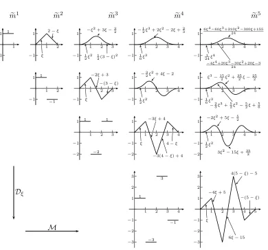
Definition 4.1 _{(Polynomial hills). Initially, define the integral operatorMby}

(_Mf)(ξ) = Z 1

0

f(ξ₋̺) d̺= Z ξ

ξ−1

f(̺) d̺

for any integrable functionf:R_→R_{. Now fork∈}N_{>1 let the k-th polynomial hill}

be

e

mk:=_Mm_ek−1

based on the rectangular functionm_e1 given bym_e1(ξ) = 1forξ _∈[0,1[andm_e1(ξ) = 0

Actually, m_e1 =_Mm_e0 if we let m_e0 =δ be the ‘left lopsided’ Dirac delta distribution defined by its integral R_−∞ξ δ(t) dt being 0 for ξ <0 and 1 for ξ _≥0. Contrastingly, the standard Dirac delta function is balanced and hasR_−∞0 δ(t) dt= 1₂. However, we will stick to the lopsided variant throughout the entire paper. By _Dξ we denote the differential operator with respect toξ .

Lemma 4.2 _{(Polynomial hills).}

(i) m_ek(ξ) = 0 for ξ <0 or ξ_≥k.

(ii) m_ek_{(ξ) =} 1

(k−1)!ξk−1 forξ ∈[0,1[andmek(ξ) = (k−11)!(k−ξ)k−1forξ ∈[k−1, k[.

(iii) m_ek restricted to [j, j+ 1[ is a polynomial function of degree k ₋1 for j _∈

{0, . . . , k₋1_}. In particular,m_ek is smooth for ξ_∈R_{\ {0, . . . , k}.}

(iv) m_ek _{is(k−2)-fold continuously differentiable.}

(v) Conversely, the conditions (i) through (iv) uniquely determine m_ek.

(vi) _Dξim_ek =_MDi_ξm_ek−1 as long as i_≤k₋2 and even fori=k₋1 when read for distributions.

(vii) The function m_ek is symmetric to k₂: m_ek(ξ) =m_ek(k₋ξ).

(viii) Forξ_∈[j, j+ 1[ (corresponding to case(k, j)) we have

Dkξ−1mek(ξ) = (−1)j ·

_k

−1 j

.

(ix) The next derivate can only be correctly described as a linear combination of Dirac delta distributions:

Dkξmek(ξ) =

X

0≤j≤k

(₋1)j

k j

·δ(ξ₋j).

(x) For any 0_≤ℓ < k we obtain the following explicit description:

Dξℓmek(ξ) =

1 (k₋1₋ℓ)!

X

0≤i≤⌊ξ⌋

k i

(₋1)i(ξ₋i)k−1−ℓ

e m1 1 −1 1 1 e m2 1 −1 1 2 ξ

2−ξ

1 −1 1 2 1 −1 e m3 1 −1

1 2 3

1

2ξ2

−ξ2+ 3ξ−3₂

1

2(3−ξ)2

1

−1

1 2 3 ξ

−2ξ+ 3 −(3−ξ)

1

−1

−2

1 2 3 1 −2 1 e m4 1 −1

1 2 3 4

1

6ξ3

−1₂ξ3+ 2ξ2−2ξ+2₃

1

−1

1 2 3 4

1

2ξ2

−3₂ξ2+ 4ξ−2

1

−1

−2

1 2 3 4

ξ

−3ξ+ 4

−3(4−ξ) + 4 4−ξ

1 2 3 −1 −2 −3

1 2 3 4

1 −3 3 −1 e m5 1 −1

1 2 3 4 5

1

24ξ4

−4ξ4+20ξ3−30ξ2+20ξ−3

24

6ξ4−60ξ3+210ξ2−300ξ+155

24

1

−1

1 2 3 4 5

1

6ξ3

−2₃ξ3+5₂ξ2−5₂ξ+5₆ ξ3−152ξ

2₊35

2ξ−

25 2

1

−1

−2

1 2 3 4 5

1

2ξ2

−2ξ2+ 5ξ−5₂

3ξ2−15ξ+35 2 1 2 3 −1 −2 −3

1 2 3 4 5

ξ

−4ξ+ 5

6ξ−15 4(5−ξ)−5

−(5−ξ)

M Dξ

Figure 4.1: Graphs of the polynomial hills m_ek _{for k≤5 and their derivatives}

Curiosity: The function√k_·m_ekcan also be described as the volume of a slice through a(k₋1)-dimensional unit hypercube of thickness √1

k orthogonal to a main diagonal.

That’s the same as saying it is √1

k times the (k−1)-volume of the cut between a

k-dimensional hypercube and the hyperplaneP_1≤i≤k̺i =ξ. This last interpretation

makes it obvious that _Z

k

0 e

mk(ξ) dξ= 1, since this is the volume of thek-hypercube.

Proof. _{From the definition (i) through (vii) follow directly. Further, note that}

k >1. The recursion form_e differentiated k₋1times yields forξ _∈[j, j+ 1[

Dξk−1mek(ξ) =DξMDξk−2mek−1(ξ)

=_Dξk−2m_ek−1(ξ)_{− Dξ}k−2m_ek−1(ξ₋1)

= (₋1)j

k₋2 j

−(₋1)j−1

k₋2 j₋1

= (₋1)j

k₋1 j

.

(ix) follows similarly.

To prove (x) consider h(ξ) = _(k−1_1)!P_{0≤i≤⌊ξ⌋} k_i(₋1)i_(ξ−i)k−1_{. ThenD}k−1

ξ h= Dξk−1mek using (viii). And obviously Dξℓh(0) = 0 = Dξℓmek(0) for 0 ≤ ℓ < k−1, so

that inductively (with fallingℓ) we get _Dξℓh=_Dξℓm_ek.

As we do not need (v) and (xi), we leave these proofs to the interested reader.

Most of the following is easier if we first renormalize λek_{. So we let}

e

λk_normhξ_i:= 1 αk_Bk+ξαλe

k hξ_i. (4.3)

The recursion foreλk _{now turns into}

e

λk_norm=_Meλk_norm−1 .

Theorem 4.4 _{(Approximation order). For any ξ∈}R_{we have}

e

λk_normhξ_i= Z ξ

0

B−̺αm_ek(ξ₋̺) d̺=B−ξα Z ξ

0

B̺αm_ek(̺) d̺ ,

e

λk_normhξ_i= 1 (₋αlnB)k



 X

0≤i≤⌊ξ⌋ _k

i

(₋1)iB−(ξ−i)α

− X

0≤ℓ≤k−1

(₋αlnB)ℓ_{· Dξ}k−ℓ−1m_ek(ξ)  ,

e

λk_normhξ_i= X

0≤i≤⌊ξ⌋

k i

(₋1)icutexpk(−(ξ−i)αlnB) (₋αlnB)k ,

where cutexp_k(ζ) =exp(ζ)₋P_{0≤ℓ≤k−1}ζ_ℓℓ_! =P_ℓ≥kζ_ℓℓ_!. We can also express cutexp_k

Proof. _{The definition for}e_λ0 _{turns into}

e

λ0_normhξ_i= Z _∞

0

B−̺αδ(ξ₋̺) d̺ .

Now, since_Mcommutes with this integration this immediately implies that e

λk_normhξ_i= Z _∞

0

B−̺αm_ek(ξ₋̺) d̺

which is the first stated equality noting that m_ek is zero outside [0, k]. By partial integration we obtain

e

λk_normhξ_i= 1 αlnBme

k_(ξ)− 1

αlnB Z _∞

0

B−̺α_Dξm_ek(ξ₋̺) d̺

= X

1≤i≤k

(₋1)i−1

(αlnB)iD

i−1

ξ mek(ξ) +

(₋1)k

(αlnB)k Z _∞

0

B−̺α_Dξkm_ek(ξ₋̺) d̺ .

Using the description of _Dk_ξm_ek from Lemma 4.2(ix) the last integral turns into the claimed sum of the second stated equality. Expressing _Dk_ξ−ℓ−1m_ek(ξ ₋̺) us-ing Lemma 4.2(x) and rearrangus-ing slightly yields the third equality.

We are going to estimate the estimation of the error in the next section. To that aim we first need to estimateλek_norm. If k >0 then, based on Theorem 4.4 and

e

mk_{(ξ)≤1, we obtain the upper bound}

e

λk_normhξ_i= Z _∞

0

B−̺αm_ek(ξ₋̺)d̺_≤ 1 αlnB.

For k = 0 we have λe0_normhξ_i = B−ξα for ξ _≥0 and so eλ0_normhξ_{i ≤} 1 will do for all ξ_∈R_.

We first describe the qualitative behaviour of eλk_norm. Actually its graph looks like a slighty biaswise hill.

Lemma 4.5. _{The function λ}ek

normhξi=B−ξα

Rξ

0 B̺αmek(̺) d̺ is zero at ξ = 0, posi-tive atξ =k, more precisely

e

λk_normhk_i= ₁

−B−α

αlnB k

,

and there is a position ξk1 2 ∈

]0, k] such that it is increasing on]0, ξk1 2

[and decreasing

on]ξk1 2

, ξ[. Further, ξk1 2 ≥

k

Proof. _{First, inspecting}

e

λ1_normhξ_i= Z ξ

0

B−̺αm_e1(ξ₋̺) d̺

=     

0 if ξ <0,

1−B−ξα

αlnB if ξ∈[0,1],

1−B−α

αlnB B−(ξ−1)α if ξ >1. 0 1

1−B−α

αlnB

shows that for k= 1 all claims hold with ξk 1 2

= 1. So in the remainder of this proof we assumek >1.

Next, computeλek_normhk_i inductively:

e

λk_normhk_i=B−kα Z k

0

B̺α Z 1

0 e

mk−1(̺₋̺k) d̺k d̺

=B−α Z 1

0

B̺kα d̺k

| {z }

=1−B−α αlnB

·B−(k−1)α Z k−1

0

Bτ αm_ek−1(τ) dτ

| {z }

=λek−1

normhk−1i

=

1₋B−α

αlnB k

.

Here we have substituted τ = ̺ ₋̺k and collapsed the new integration interval

[₋̺k, k−̺k]for τ to [0, k−1]sincemek−1 vanishes on the difference Moreover, based

onλek

normhξi=B−ξα

Rξ

0 B̺αmek(̺) d̺ we obtain

Dξλek_normhξ_i=₋αlnB_·eλk_normhξ_i+m_ek(ξ), (4.6)

and infer that_Dξeλk_normhk_i=₋αlnB1_α−_lnB−_Bαk is negative. Finally, compute the derivate ofeλk

norm differently

Dξeλk_normhξ_i=_Dξ Z ξ

0

B−̺αm_ek(ξ₋̺) d̺

=B−ξα Z ξ

0

B̺α_Dξm_ek(̺)d̺ .

The integral kernel B̺α_Dξmek_{(̺) is positive on ]0,}k

2[ and negative on ]k2, k[. Thus

Rξ

0 B̺αDξmek(̺) d̺ increases on ]0,k2[and decreases on]k2, k[. Since this term starts

at zero, it is positive for some time, begins to decrease at k₂, traverses zero at some pointξk1

2

recalling that atkthe value is negative, and stays negative tilξ =ksince it continues to decrease. Thus the sign of_Dξλek

normhξiis positive on]0, ξk1 2

[and negative on]ξk1

2

, k[, and soeλk_normhξ_i is increasing till ξk1 2

0 1 2 3 4 5 6 7 1−B−α

αlnB

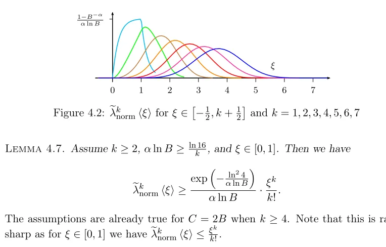
ξ

Figure 4.2: eλk_normhξ_ifor ξ _∈−1₂, k+ 1₂and k= 1,2,3,4,5,6,7

Lemma 4.7. _{Assume k≥2, αlnB ≥} ln16

k , and ξ∈[0,1]. Then we have

e

λk_normhξ_{i ≥}

exp_−αln_ln24_B αlnB ·

ξk k!.

The assumptions are already true for C = 2B when k_≥4. Note that this is rather sharp as forξ_∈[0,1]we haveλek_normhξ_{i ≤} ξ_kk_!.

Proof. _{We use the integral representation from Theorem 4.4 and estimate the} polynomial hill partm_ek_{(ξ−̺) of its kernel by a simple piecewise constant function}

as indicated in the picture. We obtain

e

λk_normhξ_i= Z ξ

0

B−̺αm_ek(ξ₋̺) d̺

≥

Z ε

0

B−̺α d̺_·m_ek(ξ₋ε)

= 1

αlnB 1−exp(−εαlnB)

e

mk(ξ₋ε).

B−̺α

e

mk(ξ−̺)

0 1

0 1 2

̺ ξ

ε

This holds for anyε_∈[0, ξ]since0_≤ξ_≤ k₂ ensures thatm_ekis increasing. So we can optimize εdepending on ξ. We obtain a suitable value when setting εby

1₋exp(₋εαlnB) = ξ k. (4.8)

To make sure that now ε_≤ξ we use the following simple fact. Fact 4.9. _{For any ϑ >0 andτ =} 1−exp(−ϑ)

ϑ the map

[0, ϑ] _−→ [0, τ ϑ], z _7−→ 1₋exp(₋z),

ϑ τ ϑ 1−e−z

τ z z

Let ϑ1 > 0 be such that 1−exp(−ϑ1) = _k1. Namely, ϑ1 = −ln 1−_k1. With

τ1= 1−exp(_ϑ1−ϑ1) then1 =τ1ϑ1kand _kξ ≤τ1ϑ1. Thus we haveεαlnB ∈[0, ϑ1]so that

τ1εαlnB≤1−exp(−εαlnB) =

ξ

k ≤εαlnB. (4.10)

In particular,ε_≤ξ follows fromkτ1αlnB = _ϑ1₁αlnB ≥1. By Fact 4.9 withϑ=ln2

we obtain τ = _2ln1₂ and 1_−k1k _≥ exp(₋1_τ) = exp(₋ln4) for all k _≥ 2. Thus kϑ1 = −kln 1−1_k ≤ ln4. Further, αlnB ≥ ln_k16 > ln4_k ≥ ϑ1. This now implies

ε_≤ξ.

Since ξ_∈[0,1] we have the explicit expressionm_ek(ξ₋ε) = (ξ₍−_k−ε)_1)!k−1 and so

e

λk_normhξ_{i ≥} ξ kαlnBme

k_{(ξ−ε) =} (1−ε/ξ)k−1

αlnB · ξk k!.

Sinceϑ1< αlnBwe can defineϑ2by1−exp(−ϑ2) = _αϑ_ln1_B, and according to Fact 4.9

let τ2 = 1−exp(_ϑ2−ϑ2). Combining with (4.10) gives us

1₋ε_ξk _≥ 1_−kτ 1 1αlnB

k

=

exp_−τ 1

2τ1αlnB

and thus simplifies our above inequality to

e

λk_normhξ_{i ≥}

exp_−τ 1

2τ1αlnB

αlnB · ξk

k!. (4.11)

By our choices

1 τ1τ2αlnB

=kϑ2 ≥

kϑ1

αlnB ≥ 1 αlnB.

Though these inequalities get equalities with k _{→ ∞}, we need a precise estimate. Substituting kin₋kln 1₋ 1_k≤ln4 with kα_lnln₄B yields

1 τ2τ1

=kαlnB_·ϑ2 =−kαlnBln

1₋ kϑ1 kαlnB

≤ −kα_lnln₄B ln

1₋ ln4 kαlnB

ln4_≤ln24

provided αlnB _≥ ln_k16.

Though we know the value of eλk_normhk_i, it is orders smaller than the above left lower bound. Thus let us consider eλk

Lemma 4.12. _{Ifk≥3 then forξ∈[k−1, k]we have}

e

λk_normhξ_{i ≥} (1−B−

α₎k

αlnB ·

(k₋ξ)k−1

(k₋1)! .

Proof. _{By definition we have} e_λk

normhξi =

e

λk_hξi

αk_Bk+ξα. Theorem 4.4’s third

descrip-tion expresseseλk

normon[k−1, k]as a sum ofkterms. Adding the missing termi=k

we obtain _αkλe_Bkhkk+iξα, noting that eλk is constant forξ > k:

e

λk_normhξ_i=

1₋B−α

αlnB k

B(k−ξ)α₋cutexpk((k−ξ)αlnB) (αlnB)k

To check the claimed inequality we substitute τ = (k₋ξ)αlnB _∈[0, αlnB] (elimi-natingξ):

e

λk_normhξ_i= P

0≤ℓ≤k−1 τ

ℓ ℓ! −

1₋(1₋B−α)keτ

(αlnB)k .

We have to show that this is at least (1−B−α)k

(αlnB)k

τk−1

(k−1)! which we rewrite to

X

0≤ℓ≤k−2

τℓ ℓ! ≥

1₋(1₋B−α)k eτ₋ τ

k−1

(k₋1)!

.

Obviously(1₋B−α₎k _≥(1−e−τ₎k _{in our situation, with equality for τ =αlnB or}

ξ=k₋1. Thus it suffices to show for any τ >0 X

0≤ℓ≤k−2

τℓ

ℓ! ≥(1−(1−e −τ₎k₎

eτ₋ τ

k−1

(k₋1)!

. (4.13)

The remaining proof proceeds in four steps:

◦ High case: P_{0≤ℓ≤k−2} τ_ℓℓ_{! ≥}k.

◦ Low case: 1−_τe−τ _≥ qk 1+σ

k! , where 1σ + 1≤

ek−1_(k−1)!

(k−1)k−1 . ◦ Covering: Fixingσ := √ 1

2π(k−1)−1 these cases cover allτ >0 if k≥4.

◦ Brute-force: Prove (4.13) fork= 3. (Actually, for k_{∈ {}3,4,5,6,7,8,9_}.) High case: Since eτ _≥ P_{0≤ℓ≤k−2}τ_ℓℓ_{! ≥} k in this case we have τ _≥ lnk. Employing

Bernoulli’s inequality(1₋T)k_≥1₋kT for T =e−τ _≤1 we obtain (1₋(1₋e−τ)k)

eτ₋ τ

k−1

(k₋1)!

≤ke−τ

eτ ₋ τ

k−1

(k₋1)!

=k

1₋ τ

k−1

(k₋1)!e −τ

≤k_≤ X

0≤ℓ≤k−2

τℓ

As Bernoulli’s inequality is good forT close to 0 only, it is not surprising that this only gives a sufficient result forτ large enough.

Low case: Assume 1−_τe−τ _≥ qk 1+σ

k! where σ is chosen such that σ1 + 1 <

ek−1_(k−1)!

(k−1)k−1 .

(Since 1−e_τ−τ is decreasing, this is always true on some interval[0, τ0].)

The condition on σ implies that eτ₋ 1_σ + 1₍τ_k−k−_1)!1 is non-negative for all τ >0: Considerf0(τ) = e

τ_(k−1)!

τk−1 − _σ1 + 1

. Then f₀′ vanishes at τ =k₋1 only and thusf0

is minimal there. The assumption onσ is precisely f0(k−1)≥0.

Further, note that ₍τ_kk₋−_2)!2 + _(kτk₋−_1)!1 _≤ eτ _≤ P_{0≤ℓ≤k−1} τ_ℓℓ_! +eτ τ_kk_!. We use this to obtain:

1₋(1₋e−τ)k | {z } ≥(1+kσ!)τ k

eτ₋ τ

k−1

(k₋1)!

| {z }

≥0

≤eτ ₋ τ

k−1

(k₋1)! −(1 +σ) τk k!e

τ_{+ (1 +σ)}τk

k! τk−1 (k₋1)!

≤ X

0≤ℓ≤k−2

τℓ ℓ! −

στk k! e

τ _{+ (1 +σ)}τk

k! τk−1 (k₋1)!

= X

0≤ℓ≤k−2

τℓ ℓ! −σ

τk k!

eτ₋

1 σ + 1

τk−1 (k₋1)!

| {z }

≥0

≤ X

0≤ℓ≤k−2

τℓ ℓ!.

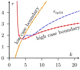
Notice that the value ofσ only influences the set of values ofτ that fall in this case. Covering: We chooseσ := √ 1

2π(k−1)−1. Recall Stirling’s formula: For any n >0there

is a ϑ _∈ ]0,1[ such that n! = n_en√2πne12n1+ϑ_{, see Robbins (1955). We thus have}

1

σ+1 =

p

2π(k₋1)< e₍k_k−₋1(₁₎kk−−1)!1 as required. Further, we define the valueτsplitwhere

we split between the low and the high case:

τsplit:=

    

2lnk_e if k_≥8, 2 if 5_≤k_≤7,

√

7₋1 if k= 4. We start with the treatment of the casesk_≥8.

We claim that for τ _≤τsplit we are in the low case, ie.

1₋e−τ

τ ≥

k

r 1 +σ

k! =:ϑ. (4.14)

Consider f2(τ) = 1−e−τ −ϑτ. It obviously vanishes atτ = 0. The derivative off2

Coarse-grained integers 21 0 1 2 3 4

0 5 10 15 20

τ τsplit low case bou nd ary highcase boundary k b

b b b b b

b b b b

b b

b b b b b b b b b b b b b b b b

b b b b b b b b b b b b b b b b b b b b b b b b b c b

c bc bc bcbc

b c b c b c b c b c b

c bc

b

c bc

b

c bc

b

c bc

b

c bc bc

b

c bc bc

b

c bc bc

Figure 4.3: Case coverage and τsplit

prove (4.14) forτ _∈]0, τsplit]it is thus sufficient to prove that f2 is at least 0at the

right boundary. First, note that by Stirling’s formula we have k!_≥ k_ek√2π and so we can estimate ϑby _ke:

ϑ= k r

1 +σ k! ≤

e k k s 2 √ 2π | {z }

≤1

≤ _ke.

Well, now we have

k_·f2(τsplit) =k−

e2

k −kϑτsplit

≥k₋e

2

k −2e ln k

e =:f3(k).

Checking that f3(e) = 0 and the derivative f3′(k) = (1− ek)2 is positive for k > e

shows that f3(k) >0 for all k ≥ 3. Thus for τ ≤τsplit we are in the low case with

the above choice of σ.

It remains to check that forτ _≥τsplitwe are in the high case. We use the Lagrange

remainder estimate of the power series of the exponential function and again Stirling’s formula to obtain

X

0≤ℓ≤k−2

τℓ

ℓ! ≥e

τ

1₋ τ

k−1

(k₋1)!

≥eτ 1₋

eτ k₋1

k−1!

=:f5(k, τ).

As the left hand side is increasing in τ > 0 we consider the smallest τ in question: letf6(k) :=f5(k, τsplit)/k. Therein,

eτsplit

k₋1 k−1

=exp

−(k₋1) | {z }

(I)

−ln2₋1₋ln lnk

e +ln(k−1)

| {z }

(II)

Observe that the term (I) is obviously positive and increasing fork_≥8. The same is true for the term (II): its derivative _k−1_1−k(ln1_k

−1) is positive fork≥e2≈7.39 and

the value of term (II) at e2 _{is positive. Using this we infer that f}

6 is increasing and

positive. Checkingf6(10)>1(f6(10)∈]1.19,1.20[) now provesP0≤ℓ≤k−2

(2lnk_e)ℓ

ℓ! ≥

kfor k_≥10. For k= 8 andk= 9 we just verify this inequality directly.

It remains to consider4_≤k_≤7. Here we use individual seperation positions as defined above:

k 4 5 6 7 (8) (9)

τsplit √7−1 2 2 2 2ln8_e 2ln9_e 1−e−τsplit

τsplit 0.49 0.43 0.43 0.43 0.40 0.37

∨ for low case

k

q

1+σ

k! 0.48 0.40 0.35 0.31 0.28 0.25

P

0≤ℓ≤k−2

τℓ

split

ℓ! 4 6.33 7.00 7.27 8.60 10.93 ≥kfor high case

Just check that for this τsplit the low and the high case conditions are both fulfilled.

Summing up: the claim is proved fork_≥4.

k <10: For k= 3 we need an explicit check as the estimates done in the low and the high case are too sloppy. As the following actually is a general computational way to verify the inequality (4.13) we do describe it in general, show computational results for 3_≤k_≤10 and make the critical case k= 3 hand-checkable at the end. For the verification we use a small trick and brute force: First, we substitute occurrences of e−τ _{with a new variableT. The task turns into showing that the bivariate polynomial}

Fk(τ, T) :=

X

0≤ℓ≤k−2

τℓ

ℓ! −

(1₋(1₋T)k₎

T

1₋ τ

k−1

(k₋1)!T

is non-negative at τ = ₋lnT for T _∈ ]0,1]. Now, observe that Fk is increasing in

τ >0 for fixed T _∈ [0,1]. If we thus replace ₋lnT with a lower bound and we can show that the resulting term is still non-negative then we are done. For T _∈ ]0,1] we have ₋lnT _≥P_1≤ℓ≤s(1−_ℓT)ℓ. This lower bound even converges to ₋lnT, which actually ensures that we can always find some sthat allows the following reduction. We consider the univariate polynomial

gk,s(T) :=Fk



 X

1≤ℓ≤s

(1₋T)ℓ ℓ , T

 .

By our reasoning, the claim follows if _∀T _∈ ]0,1] : gk,s(T) ≥0 for some s. This in

turn is implied by

gk,s(0)>0 ∧ gk,s(T) has no zero for0< T <1.

The second statement can be checked using Sturm’s theorem (Sturm 1835) by only evaluating certain rational polynomials at T = 0 and T = 1. However, this only works if the chosensis large enough. We have determined the smallest sthat make (4.15) true:

k 3 4 5 6 7 (8) (9)

s 4 3 4 5 6 7 8

deggk,s 11 13 21 31 43 57 73

time (sec) 0.19 0.29 0.60 2.8 24 235 1704 Though we can always divide out(1₋T)k _fromg

k,s the degrees are in all cases quite

high and the computations better done by a computer. The timings refer to our own (non-optimized) MuPad-program used to assert (4.15). As k = 3 is the only case that we do not cover otherwise we giveg3,4 here:

g3,4(T)/(1−T)3 =

1

12(1−T) + 5

6T+T(1−T)

481

96 (1−T)

2₊35

24T

2_+T(1

−T)

245

96 (1−T) + 103

24 T +T(1−T)

119

144(1−T)

2₊ 89

144T

2_+T(1−T)·407

288

With this description you can easily see that it is positive on[0,1[. Finally, we put together the upper bound oneλk_norm, Lemma 4.5, Lemma 4.7, and Lemma 4.12 in the following theorem.

Theorem 4.16. _{For any k≥1 we have}

e

λk_normhξ_{i ≤e}ck:=

( ₁

αlnB if k >0,

1 if k= 0.

Assume αlnB _≥max ln2,ln_k16. Then for any ε_∈]0,1] withε_≤k₋ξk1 2

or k < 3

there is ac˘k >0such that for ξ ∈[ε, k−ε]

e

λk_normhξ_{i ≥} ˘ck αlnB.

Here we can choose

˘

ck=min

2−4_·ε

k

k!, 2

−k_· εk−1

(k₋1)!

Note thatξk1 2

is the maximum ofeλk_normwhich in our experiments is always less thenk₋ 1fork_≥3. However, proving that would result in a stronger version of Lemma 4.12, which even in the given form required quite some effort. However, we just want that to work for some small εand that is always granted.

Proof. _{The upper bound being proven we consider the lower bound. First, keeping} in mind that αlnB _≥ln2 andαlnB _≥ ln_k16, we consider the cases k_≥3. We know by Lemma 4.5 thateλk

normon[ε, k−ε]attains its minimal value at one of the boundaries

since ξk1 2 ∈

[ε, k ₋ε] (by assumption). We thus only need to consider its values at ξ=ε and atξ=k₋ε.

On the left hand side Lemma 4.7 gives

αlnB_·eλk_normhε_{i ≥}exp

− ln

2₄

αlnB

εk

k! ≥exp

−ln

2₄

ln2

εk

k! = 2 −4_·εk

k!

using the conditions onαlnB.

On the right hand side by Lemma 4.12 we find

αlnB_·eλk_normhk₋ε_{i ≥}(1₋exp(₋αlnB))k ε

k−1

(k₋1)! ≥2

−k εk−1

(k₋1)!

using again αlnB _≥ln2. This completes the proof for the casesk_≥3.

We will now show corresponding lower bounds for the cases k= 1,2. For k= 1 we have forε_∈]0,1] usingαlnB _≥ln2:

αlnB_·λe1_normhε_i= 1₋exp(₋εαlnB)_≥1₋exp(₋εln2). Using Fact 4.9 and ε_≤1, we have

1₋exp(₋εln2)_≥ 1−exp(−ln2) ln2 ε=

1 2ln2ε≥

1 2ε.

Fork= 2 we again apply Lemma 4.7 for the left hand side as in the general case. For the right hand side we show that

α2ln2B_·λe2_normh2₋ε_{i ≥}

1₋ 1 2ln2

εαlnB

for0_≤εαlnB _≤αlnB, ln2_≤αlnB. Since 1_−2ln1_2≥2−2 this proves the claim. Now, using Theorem 4.4 we write the left hand side minus the right hand side as f5(εαlnB, αlnB) withf5(τ, ϑ) =exp(τ −2ϑ)−2exp(τ −ϑ) +_2ln21 τ + 1. We have

to show thatf5 is non-negative if0≤τ ≤ϑandϑ≥ln2. Theϑ-derivative of f5,

∂f5

is positive forϑ >0. Thus it suffices to show thatf5(τ, ϑ)≥0for the smallest allowed

ϑ, which is the larger ofτ and ln2. Ifτ _≥ln2then we considerf5(τ, τ) =exp(−τ) + 1

2ln2τ −1. This expression is increasing in this case (even for τ ≥ln2 +ln ln2) and

so it is greater than or equal tof5(ln2,ln2) = 0. If otherwise 0 ≤τ ≤ln2 then we

considerf5(τ,ln2) =−3₄exp(τ) +_2ln1₂τ + 1which is decreasing even for τ ≥0 and

so it is greater than or equal tof5(ln2,ln2) = 0.

Summing up we obtain:

Corollary 4.17. _{For any ε ∈ ]0,1] and any k ≥ 1 we have uniformly for ξ ∈}

[ε, k₋ε]

e

λk_normhξ_{i ∈}Θ

₁

αlnB

.

5. Estimating the estimate bλk

The recurrence Lemma 3.6 for bλk _{is more complex than the one for eλ}k_{, so instead}

of solving it we estimate it. We consider also here the normed version bλk_normhξ_i :=

b

λk_hξi

αk_Bk+ξα. To better understand how the error behaves we compute it for k= 1:

b

λ1_normhξ_i=       

0 if ξ_∈]_−∞,0[,

1+ξα

8πα lnB B12 +ξα2

+_8πα1 lnB

B12 +ξα if ξ∈[0,1[,

1+α

8πα_B1lnB 2−α_{2 +}ξα +

1 8πα_Bln1B

2 +ξα if ξ∈[1,∞[.

From this we estimatebλ1

norm directly:

b

λ1_normhξ_{i ≤}     

0 if ξ _∈]_−∞,0[,

(2+α)lnB

8πα B− 1+ξα

2 ifξ ∈[0,1[,

(1+α)lnB

8πα B− 1

2+α2−ξα+lnB

8πα·B− 1

2−ξα ifξ ∈[1,∞[.

We have also looked at precise expressions for largerk, yet they are huge and do not give rise to better bounds.

Theorem 5.1. _{Define values bck recursively by}

b

ck:=bck−1+

4 + 3lnB

8πα√B (eck−1+bck−1)

for k_≥3 based on _bc0 := 0, bc1:= (2+_8παα)√ln_BB, and

b c2 :=

6 + 3α 8πα2

1

√

B +

4 + 3lnB

8πα√B (ec1+bc1)

= 9 + 3α 8πα2

1

√

B +

1

2πα2√_BlnB +

Then for any kand ξ_∈R_{we have}

b

λk_normhξ_{i ≤b}ck

Ifα_≥ ln√B

B we have for k≥2 and largeB the inequality

b ck≤

(2k₋1)(1 +α) α2√_B .

For k = 1 the order of _bc1 is necessarily slightly larger. More precisely, we have for largeB that

b c1≤

(1 +α)lnB α√B .

Instead of defining_bc2 and bc1 we could have left that to the recursion. But the given

values are smaller than the ones derived from the recursion based on _bc0 only. For

k= 1 the recursion would give 4+3lnB

8πα√B. For k≥2 however the improvement due to

these explicit settings is a factor of order lnB.

Proof. _{We first show that the valuebckis bounded as claimed. Fork= 1the claim} follows directly from the definition, since we have forB >exp(1)that(2 +α)lnB_≤ 2(1 +α)lnB asα is positive. Fork= 2we have for ln2B _≤√B the inequality

b c2 =

6 + 3α 8πα2

1

√

B +

4 + 3lnB

8πα√B (ec1+bc1)

≤ 1 +α

α2√_B +

1 α2√_B +

(1 +α)ln2B α2_B

≤ 3(1 +α)

α2√_B .

Fork_≥2we proceed inductively. We have b

ck=bck−1+

4 + 3lnB

8πα√B (eck−1+bck−1)

≤ (2

k−1_{−1)(1 +α)}

α2√_B +

lnB α√B

1 αlnB +

(2k−1₋1)(1 +α) αlnB

= (2

k_{−1)(1 +α)}

α2√_B .

Now we prove the remaining estimate by induction onk. The casek= 0is true by definition ofλb0_{(with equality). Fork= 1the inspection above proves the claim. The}

case. So assumek_≥3. Using the definition of bλk from Lemma 3.6 we split bλk into three summands:

b

λk_normhξ_i= Z 1

0

b

λk_norm−1 _hξ₋̺_i d̺

+2Eb(B) αB ·(eλ

k−1

norm+λbknorm−1 )hξi

+ Z 1

0

(eλk_norm−1 +bλk_norm−1 )_hξ₋̺_iEb′(B1+̺α)lnB d̺ .

ForEb(x) = ₈1_π√xlnx we calculate as a preparative 2Eb(B)

αB = lnB 4πα√B, (5.2)

Z 1

0

b

E′(B1+̺α)lnB d̺= 4 +lnB 8πα√B −

4 +lnC 8πα√C. (5.3)

The first summand of bλk

norm is at most bck−1 by induction hypothesis. The second

summand we estimate using (5.2) by lnB

4πα√B(eck−1+bck−1).

The third summand is bounded by

(_eck−1+bck−1)

Z 1

0

b

E′(B1+̺α)lnB d̺ .

By (5.3) the third summand is at most 4 +lnB

8πα√B (eck−1+bck−1).

This completes the proof of the casek_≥3: b

λk_normhξ_{i ≤b}ck−1+

lnB

4πα√B(eck−1+bck−1) +

4 +lnB

8πα√B (eck−1+bck−1) =_bck.

prove. Forξ_∈[0,1[we find for this first summand Z ξ

0

b

λ1_normhξ₋̺_i d̺_≤ Z ξ

0

(2 +α)lnB 8πα B−

1 2−

(ξ−̺)α 2 d̺ = (2 +α)lnB

8πα B

−1 2 B−

ξα 2

Z ξ

0

B̺α2 d̺

| {z }

=_αln2_B

1−B−ξα₂

≤ 2 +α

4πα2√_B.

Forξ_∈[1,2]we find Z 1

0

b

λ1_normhξ₋̺_i d̺_≤ Z 1

ξ−1

(2 +α)lnB 8πα B−

1 2−

(ξ−̺)α 2 d̺ +

Z ξ−1

0

b

λ1_normh1_iB1+αB−(1+(ξ−̺)α) d̺

= (2 +α)lnB 8πα B−

1 2−

(ξ−1)α 2 B−

α 2

Z 1

ξ−1

B̺α2 d̺

| {z }

=_αln2_B

1−B−(2−₂ξ)α

+λb1_normh1_iB−(ξ−1)α Z ξ−1

0

B̺α d̺

| {z }

=_αln1_B(1−B−(ξ−1)α₎

≤ 2 +_4παα₂B−12− (ξ−1)α

2 + 1 +α 8πα2B−

1 2−

α 2 + 1

8πα2B−

1 2−α

≤ 6 + 3α

8πα2√_B

As bλ1

norm decreases for ξ ≥ 1 this bound also holds for ξ ≥ 2. Putting everything

together the above defined value_bc2 boundsλb2normhξias claimed.

It is tempting to guess that we can save more lnB factors for larger k. How-ever, inspecting bλ2

norm shows that, say, bλ3norm

₁

2

∈Ω√1

B

. (For ξ _∈[0,1[ we find b

λ2

normhξi= _4πα3√_B+O

1

√

BlnB

.)

6. Reestimating λbk _{without Riemann}

Fact 6.1. _{◦ Forx >10 we have}

|π(x)₋Li(x)_{| ≤}11.88x(lnx)35 exp

−₅₇1 (lnx)35(ln lnx)− 1 5

.

◦ There is a constantC and a frontier x0 such that for x > x0 we have

|π(x)₋Li(x)_{| ≤}C xexp₋0.2098(lnx)35(ln lnx)−15

.

Admittedly, these bounds only start to be meaningful at large values of x (eg. the first statement around10159 299_{). All those bounds are of the form: For all x > x}

0

|π(x)₋Li(x)_{| ≤}C x(lnx)c0_{exp −A(lnx)}c1_{(ln lnx)}−c2

| {z }

=:Eb(x)

holds. Here, C >0,x0 >0,c0 ∈R,c1 >0,c2 >0 and A >0 are given parameters

(which are not always known). Note that we have that b

E(x)_/x

is decreasing for large x. Actually, with the parameter sets from Fact 6.1 this is already true forx_≥5. Moreover, the quotient of the relative errors atx1+αand atx

b

E(x1+α₎lnx1+α x1+α

b

E(x)ln_xx =

(1 +α)Eb(x1+α) xα_Eb_(x)

is bounded (or even tends to zero) with x _{→ ∞} for any α > 0. This follows from b

E(x)_{/x decreasing when α is constant, but you may also consider values for α that} increase when xgrows.

Revisiting the proof of Theorem 5.1 shows that only (5.2), (5.3), and the initial values_bc1 andbc2 depend on the specific boundE. We now use the following recursionb

for the bounds: b

ck:=bck−1+

2Eb(B) αB +

Z 1

0

b

E′(B1+̺α)lnB d̺ !

| {z }

=:u

(_eck−1+bck−1)

for k_≥1 based on _bc0 = 0, and possibly values forbc1 and bc2.

To bound u tightly the trickiest step is bounding the integral. As our interests lie elsewhere we take the easy way out. We integrate by parts and use that Eb(x)_/x is decreasing for the following rough estimate

Z 1

0

b

E′(B1+̺α)lnB d̺= Eb(B

1+α₎

αB1+α −

b E(B)

αB +lnB Z 1

0

b

E(B1+̺α₎

B1+̺α d̺

| {z }

≤Eb(BB)

Thusu is bounded by

u_≤ 1 + 1

αlnB 1 + b

E(B1+α) Bα_Eb(B)

| {z }

bounded

!! b

E(B)lnB

B .

In the following we neglect the bounded term, as we can compensate its effect for example by a small additional factor. Since u is small for large B, we expect _bck to

be dominated by_bc1 =u. Precisely, for k >1 we havebck = (1 +u)bck−1+_αlnu_B, thus

b

ck= (1 +u)k−1u+

(1 +u)k−1₋1 αlnB ∼

1 + k−1 αlnB

u.

Theorem 6.2. _{Assume that E}b_{(x) bounds |π(x)−Li(x)| and E}b_{(x)/x is decreasing}

for x > x0 and the relative error decreases fast, ie.

b

E(x1+α)ln_xx1+1+αα

b

E(x)ln_xx =

(1 +α)Eb(x1+α₎

xα_Eb_(x)

is bounded under the chosen behavior ofα. Then for anyk_≥2 andB large we have

b

λk_normhξ_{i ∈ O} 1 + k−1

αlnB 1 + 1 αlnB

bE(B)lnB B

!

for k_≥2.

This is close to optimal, we only loose a factor of order lnB in the relative error compared to the used error bound in the prime number theorem:

b λk

normhξi

e λk

normhξi

≤ 1 + k−1

αlnB

1 +_αln1_BEb(B_B)lnB

˘

ck αlnB

∼ α

˘ ck

lnB_·Eb(B)lnB

B .

The assumptions onEbalso hold for explicit error bounds withEb(x)_{∈ O} x

lnℓ_x

. Due to the lost lnB the result is only meaningful if ℓ_≥3, so Rosser & Schoenfeld (1962) does not suffice. From Dusart (1998) we can useEb(x) = 2.3854 x

ln3x for x >355 991,

and obtain

b

λk_normhξ_{i ∈ O 1}

lnB