Soft Computing Technique Based Economic Load Dispatch Using Improved Particle Swarm Optimization

Soft Computing Technique Based Economic Load

Dispatch Using Improved Particle Swarm

Optimization

Bangbang Hermanto1, Wendhi Yuniarto2, Rusman Rusman3, Hardiansyah Hardiansyah4

1, 2, 3

Department of Electrical Engineering, State Polytechnic of Pontianak, Pontianak 78124, Indonesia

4

Department of Electrical Engineering, University of Tanjungpura, Pontianak 78124, Indonesia

Abstract

This paper proposes a novel optimization methodology aimed to solve economic load dispatch (ELD) problem considering valve-point effects using improved particle swarm optimization (IPSO) algorithm through the application of Gaussian and Cauchy probability distributions. The IPSO approach introduces new diversification and intensification strategy into the particles thus preventing PSO algorithm from premature convergence. To demonstrate the effectiveness of the proposed approach, the numerical studies have been performed for two different test systems, i.e. 15 and 40 generating units, respectively. The obtained results denote superiority of the proposed technique and confirm its potential to solve the ELD problems.

Keywords: Improved particle swarm optimization, economic load dispatch, valve-point effects.

1. Introduction

The increasing energy demand and decreasing energy resources have necessitated the optimum use of available energy resources. The ELD problem is one of the fundamental issues in power system planning, operation, and control, where the total required load demand is distributed among the generation units in operation. The main goal of ELD problem of electrical power generation is to minimizing total generation cost while satisfying load demand and operational constraints. Traditionally, fuel cost function of a generator is represented by single quadratic function. But a quadratic function is not able to show the practical behavior of generator. The ELD problem is a non-convex and nonlinear optimization problem. Due to ELD complex and nonlinear characteristics, it is hard to solve the problem using classical optimization methods.

Most of classical optimization techniques such as lambda iteration method, gradient method, linear programming,

Newton’s method, interior point method and dynamic programming have been used to solve the basic economic dispatch problem [1]. In the case of ELD is practically represented as a non-convex optimization problem with equality and inequalities constraints, which cannot be solved by traditional mathematical methods. Dynamic programming (DP) technique [2] can solve such types of problems, but it suffers from so-called the curse of dimensionality. Over the past few decades, as an alternative solution to the conventional mathematical approaches, many heuristic techniques have been developed for solving the ELD problem such as genetic algorithm (GA) [3], tabu search (TS) [4], simulated annealing (SA) [5], bacterial foraging optimization (BFO) [6], evolutionary programming (EP) [7], ant colony optimization (ACO) [8], harmony search [9], biogeography-based optimization (BBO) [10], particle swarm optimization (PSO) [11]-[14], differential evolution (DE) [15], and gravitational search algorithm (GSA) [16, 17].

Recently, a heuristic technique called as particle swarm optimization (PSO) is inspired the analogy of swarm of bird and school of fish were developed by Kennedy and Eberhart [18]. In PSO, each individual makes its decision based on its own experience together with other individual’s experiences. The individual particles are pulled stochastically toward the current individual velocity positions, their own best previous performance, and previous best performance from their neighbors [19].

PSO algorithm is a useful strategy to ensure convergence of the particle swarm algorithm. Feasibility of the proposed method has been demonstrated on two different test systems, i.e. 15 and 40 generating units. The results obtained with the proposed technique were compared with other optimization results reported in literature.

2. Problem Formulation

The purpose of the ELD problem is to find the optimal scheduling of power generations that minimizes the total generation cost while satisfying equality and inequality constraints. The fuel cost curve for any unit is assumed to be approximated by segments of quadratic functions of the active power output of the generator. For a given power system network, the problem may be described as optimization (minimization) of total fuel cost under a set of operating constraints.

∑

∑

(

)

= =

+

+

=

=

n i i i i i i n i i i

T

F

P

a

P

b

P

c

F

1 2

1

)

(

(1)

where FT is total fuel cost of generation in the system

($/h), ai, bi, and ci are the cost coefficient of the ith

generator, Pi is the power generated by the ith unit and n is

the number of generators. The cost is minimized subjected to the following constraints:

2.1 Active Power Balance Equation

The total generated power by the units must be the same as total load demand plus the total transmission loss.

Loss n

i i

D P P

P =

∑

−

=1

(2)

where PD and PLoss are the total load demand and total

transmission losses, respectively. The transmission loss can be calculated by using B matrix technique and is defined as follows: 00 1 0 1 1 B P B P B P P _i n i i j ij n i n j i

Loss =

∑∑

+

∑

+

= = =

(3)

where Bij is coefficient of transmission losses and the B0i

and B00 is matrix for loss in transmission which are

constant under certain assumed conditions.

2.2 Minimum and Maximum Power Limits

The generation output of each units must be lie between minimum and maximum limits. The corresponding inequality constraint for each generator is

P

i,min

≤

P

i

≤

P

i,max

for

i

=

1

,

2

,



,

n

(4)

where Pi,min and Pi,max are the minimum and maximum

outputs of the ith generator, respectively.

2.3 Valve-Point Effects

For more rational and precise modeling of fuel cost function, the above expression of cost function is to be modified suitably. The generating units with multi-valve steam turbines exhibit a greater variation in the fuel-cost functions [12]. These “valve-point effects” are illustrated in Fig. 1.

$/MWh MW A B C D E

A : Primary Valve B : Secondary Valve C : Tertiary Valve D : Quaternary Valve E : Quinary Valve

Fig. 1 Valve-point effect [12]

The fuel cost function with valve-point effects of the generators is usually modeled as [12]:

(

)

(

)

∑

∑

= =         − × × + + + = = n

i i i i i

i i i i i n i i i T P P f e c P b P a P F F

1 ,min

2

1 sin

)

( (5)

where FT is total fuel cost of generation in ($/h) including

valve point loading, ei, fi are fuel cost coefficients of the ith generating unit reflecting valve-point effects.

3. Particle Swarm Optimization

3.1 Overview of Particle Swarm Optimization

The PSO method was introduced in 1995 by Kennedy and Eberhart [18]. The method is motivated by social behavior of organisms such as fish schooling and bird flocking. PSO provides a population-based search procedure in which individuals called particles change their position with time. In a PSO system, particles fly around in a multi dimensional search space. During the evolutionary process, each particle adjust its position based on its own experience as well as the experience of the neighboring particles, making use of the best position encountered by itself and its neighbors.

the bird to fly in the previous direction. The cognitive component models the memory of the bird about its previous best position, and the social component models the memory of the bird about the best position among the particles. The particles move around the multidimensional search space until they find the optimal solution. The modified velocity of each agent can be calculated using the current velocity and the distance from Pbest and Gbest as given below.

(

)

(

k

)

i k k i k i k i k i

X

Gbest

r

C

X

Pbest

r

C

V

W

V

−

×

×

+

−

×

×

+

×

=

+ 2 2 1 1 1

(6) where, k i

V

velocity of individual i at iteration k

k i

X

position of individual i at iteration k W inertia weight

2 1

,

C

C

acceleration coefficients

k i

Pbest best position of individual i at iteration k

k

Gbest

best position of the group until iteration k

2 1

,

r

r

random numbers between 0 and 1

In general, the inertia weight (W) is set according to the following equation [12]:

_Iter

Iter W W W

W _×

     − − = max min max max

( ₍₇₎

where,

min max,W

W initial and final weights

max

Iter

maximum iteration number

Iter

current iteration number

The approach using (7) is called “inertia weight approach (IWA)”. By using (7), a certain velocity, which gradually gets close to Pbest and Gbest can be calculated. The current position (searching point in the solution space), each individual move from the current position to the next one by the modified velocity in (6) using the following equation:

+1

=

+

k+1 i k i k

i

X

V

X

(8) where,

1

+

k i

X current position of individual i at iteration k+1 1

+

k i

V velocity of individual i at iteration k+1

The concept of the searching mechanism of PSO using the modified velocity and position of individual i based on (6) and (8) if the value of W, C1, C2, r1, and r2 are 1, as shown

in Fig. 2.

V

ki

X

ki

V

ki 1

+

X

ki

1 +

Gbest

k

Pbest

ki

V

Pbesti

V

Gbesti

Fig. 2 Concept of modification of searching point by PSO [18]

The process of implementing the PSO is as follows:

Step 1: Create an initial population of individual with random positions and velocity within the solution space.

Step 2: For each individual, calculate the value of the fitness function.

Step 3: Compare the fitness of each individual with each

Pbest. If the current solution is better than its

Pbest, then replace its Pbest by the current solution.

Step 4: Compare the fitness of all individual with Gbest. If the fitness of any individual is better than

Gbest, then replace Gbest.

Step 5: Update the velocity and position of all individual according to (6) and (8).

Step 6: Repeat steps 2-5 until a criterion is met.

3.2 Improved Particle Swarm Optimization

In recent research, some modifications to the standard PSO are proposed mainly to improve the convergence and to increase diversity. Coelho and Krohling [20] proposed the use of truncated Gaussian and Cauchy probability distribution to generate random numbers for the velocity updating equation of PSO. The proposed IPSO technique is based on Gaussian probability distribution (Gd) and Cauchy probability distribution (Cd). In this new approach, random numbers are generated using Gaussian probability function and/or Cauchy probability function in the interval [0, 1].

The Gaussian distribution (Gd), also called normal

importance of the Gaussian distribution is due in part to the central limit theorem. Since a standard Gaussian distribution has zero mean and variance of value one, it helps in a faster convergence for local search.

Here the Cauchy distribution Cd, is used to generate

random numbers in the interval [0, 1], in the social part and Gaussian distribution Gd, is used to generate random numbers in the interval [0, 1] in the cognitive part. The modified velocity equation (6) is given by

    

  

− +

− +

⋅ =

+

) ()(

) ()(

.

2 1 1

k i k d

k i k i d

k i k

i

X Gbest C

C

X Pbest G

C V W K

V (9)

ϕ ϕ

ϕ 4

2 2

2₋ − − =

K (10)

where

ϕ

=

C

₁

+

C

₂

,

ϕ

>

4

The convergence characteristic of the system can be

controlled by

ϕ

. In the constriction factor approach

(CFA),

ϕ

must be greater than 4.0 to guarantee stability.

However, as

ϕ

increases, the constriction factor K

decreases and diversification is reduced, yielding slower response. Typically, when the constriction factor is used,

ϕ

is set to 4.1 (i.e. C1, C2 = 2.05) and the constant

multiplier K is thus 0.729.

4. Simulation Results

In order to demostrate the efficiency of the proposed technique, two different power systems were tested: (1) 15-unit system considering transmission loss and valve-point effects; and (2) 40-unit system with valve-point effects and transmission losses are neglected.

Test Case 1: 15-unit system

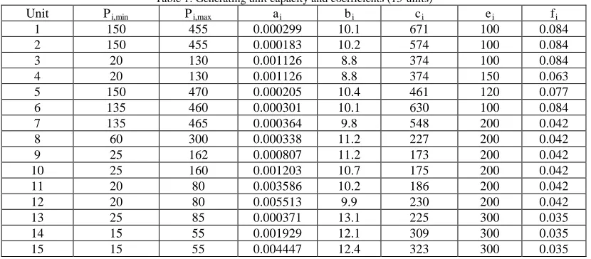
This system consists of 15 generating units and the input data of 15-generator system are given in Table 1 [11], [21]. Transmission loss B-coefficients are taken from [21]. In order to validate the proposed IPSO method, it is tested with 15-unit system having non-convex solution spaces, and the load demand is 2630 MW.

The best fuel cost result obtained from proposed IPSO and other optimization algorithms are compared in Table 2 for load demands of 2630 MW. In Table 2, generation outputs and corresponding fuel cost and losses obtained by the proposed IPSO are compared with those of GA and PSO [21]. The proposed IPSO provides better solution (total

generation cost of 30320.7233 $/h and power loss of

30.4039 MW) than other methods while satisfying the system constraints. We have also observed that the solutions by IPSO always are satisfied with the equality and inequality constraints.

Test Case 2: 40-unit system

This system consisting of 40 generating units and the input data for 40-generator system is given in Table 3 [7]. The total demand is set to 10500 MW.

The obtained results for the 40-unit system using the proposed IPSO technique are given in Table 4 and the results are compared with other methods reported in literature, including PSO, PPSO, APPSO and GSA [17, 22]. It can be observed that the proposed technique can get total generation cost of 121031.1225$/h, which is the best solution among all the methods. These results show that the proposed methods are feasible and indeed capable of acquiring better solution.

Table 1: Generating unit capacity and coefficients (15-units)

Unit Pi,min Pi,max ai bi ci ei fi

1 150 455 0.000299 10.1 671 100 0.084

2 150 455 0.000183 10.2 574 100 0.084

3 20 130 0.001126 8.8 374 100 0.084

4 20 130 0.001126 8.8 374 150 0.063

5 150 470 0.000205 10.4 461 120 0.077

6 135 460 0.000301 10.1 630 100 0.084

7 135 465 0.000364 9.8 548 200 0.042

8 60 300 0.000338 11.2 227 200 0.042

9 25 162 0.000807 11.2 173 200 0.042

10 25 160 0.001203 10.7 175 200 0.042

11 20 80 0.003586 10.2 186 200 0.042

12 20 80 0.005513 9.9 230 200 0.042

13 25 85 0.000371 13.1 225 300 0.035

14 15 55 0.001929 12.1 309 300 0.035

Table 2: Best solution of 15-unit systems

Unit power output GA [21] PSO [21] IPSO

P1 (MW) 415.3108 439.1162 455.0000

P2 (MW) 359.7206 407.9729 363.1539

P3 (MW) 104.4250 119.6324 71.3987

P4 (MW) 74.9853 129.9925 75.1350

P5 (MW) 380.2844 151.0681 364.5806

P6 (MW) 426.7902 459.9978 408.7329

P7 (MW) 341.3164 425.5601 403.8775

P8 (MW) 124.7876 98.5699 108.0356

P9 (MW) 133.1445 113.4936 66.1967

P10 (MW) 89.2567 101.1142 133.1241

P11 (MW) 60.0572 33.9116 53.7672

P12 (MW) 49.9998 79.9583 40.5174

P13 (MW) 38.7713 25.0042 39.7611

P14 (MW) 41.4140 41.4140 54.6636

P15 (MW) 22.6445 36.6140 22.4498

Total power output (MW) 2668.2782 2662.4306 2660.4039 Total generation cost ($/h) 33113.0 32858.0 30320.7233

Power loss (MW) 38.2782 32.4306 30.4039

Table 3: Generating unit capacity and coefficients (40-units)

Unit Pi,min Pi,max ai bi ci ei fi

1 36 114 0.00690 6.73 94.705 100 0.084

2 36 114 0.00690 6.73 94.705 100 0.084

3 60 120 0.02028 7.07 309.54 100 0.084

4 80 190 0.00942 8.18 369.03 150 0.063

5 47 97 0.01140 5.35 148.89 120 0.077

6 68 140 0.01142 8.05 222.33 100 0.084

7 110 300 0.00357 8.03 287.71 200 0.042

8 135 300 0.00492 6.99 391.98 200 0.042

9 135 300 0.00573 6.60 455.76 200 0.042

10 130 300 0.00605 12.9 722.82 200 0.042

11 94 375 0.00515 12.9 635.20 200 0.042

12 94 375 0.00569 12.8 654.69 200 0.042

13 125 500 0.00421 12.5 913.40 300 0.035

14 125 500 0.00752 8.84 1760.4 300 0.035

15 125 500 0.00708 9.15 1728.3 300 0.035

16 125 500 0.00708 9.15 1728.3 300 0.035

17 220 500 0.00313 7.97 647.85 300 0.035

18 220 500 0.00313 7.95 649.69 300 0.035

19 242 550 0.00313 7.97 647.83 300 0.035

20 242 550 0.00313 7.97 647.81 300 0.035

21 254 550 0.00298 6.63 785.96 300 0.035

22 254 550 0.00298 6.63 785.96 300 0.035

23 254 550 0.00284 6.66 794.53 300 0.035

24 254 550 0.00284 6.66 794.53 300 0.035

25 254 550 0.00277 7.10 801.32 300 0.035

26 254 550 0.00277 7.10 801.32 300 0.035

27 10 150 0.52124 3.33 1055.1 120 0.077

28 10 150 0.52124 3.33 1055.1 120 0.077

29 10 150 0.52124 3.33 1055.1 120 0.077

30 47 97 0.01140 5.35 148.89 120 0.077

31 60 190 0.00160 6.43 222.92 150 0.063

32 60 190 0.00160 6.43 222.92 150 0.063

34 90 200 0.00010 8.95 107.87 200 0.042

35 90 200 0.00010 8.62 116.58 200 0.042

36 90 200 0.00010 8.62 116.58 200 0.042

37 25 110 0.01610 5.88 307.45 80 0.098

38 25 110 0.01610 5.88 307.45 80 0.098

39 25 110 0.01610 5.88 307.45 80 0.098

40 242 550 0.00313 7.97 647.83 300 0.035

Table 4: Best solution of 40-unit systems

Unit power output PSO [22] PPSO [22] APPSO [22] GSA [17] IPSO

P1 (MW) 113.116 111.601 112.579 110.2604 112.6115

P2 (MW) 113.010 111.781 111.553 105.8822 112.8864

P3 (MW) 119.702 118.613 98.751 96.5985 119.1771

P4 (MW) 81.647 179.819 180.384 161.3755 131.8259

P5 (MW) 95.062 92.443 94.389 76.0761 97.0000

P6 (MW) 139.209 139.846 139.943 118.3619 138.7205

P7 (MW) 299.127 296.703 298.937 277.7329 190.0615

P8 (MW) 287.491 284.566 285.827 282.9290 254.9897

P9 (MW) 292.316 285.164 298.381 255.8505 287.9621

P10 (MW) 279.273 203.859 130.212 198.4792 130.4386

P11 (MW) 169.766 94.283 94.385 194.7330 370.7440

P12 (MW) 94.344 94.090 169.583 261.4072 373.1686

P13 (MW) 214.871 304.830 214.617 302.8148 445.7441

P14 (MW) 304.790 304.173 304.886 363.7843 336.5109

P15 (MW) 304.563 304.467 304.547 325.7610 358.3672

P16 (MW) 304.302 304.177 304.584 382.4561 408.1342

P17 (MW) 489.173 489.544 498.452 470.1274 287.8605

P18 (MW) 491.336 489.773 497.472 451.5342 458.1819

P19 (MW) 510.880 511.280 512.816 478.0455 375.9790

P20 (MW) 511.474 510.904 548.992 500.7619 442.5035

P21 (MW) 524.814 524.092 524.652 529.9021 506.2721

P22 (MW) 524.775 523.121 523.399 515.3287 548.1050

P23 (MW) 525.563 523.242 548.895 529.2006 445.3442

P24(MW) 522.712 524.260 525.871 518.1049 538.5089

P25 (MW) 503.211 523.283 523.814 489.4889 387.6950

P26 (MW) 524.199 523.074 523.565 513.8339 484.9672

P27 (MW) 10.082 10.800 10.575 10.6119 48.6070

P28 (MW) 10.663 10.742 11.177 10.2303 61.0371

P29 (MW) 10.418 10.799 11.210 12.8966 74.8758

P30 (MW) 94.244 94.475 96.178 92.6348 96.6173

P31(MW) 189.377 189.245 189.999 187.9979 189.0000

P32 (MW) 189.796 189.995 189.924 176.9925 189.6533

P33 (MW) 189.813 188.081 189.714 184.4834 182.1303

P34 (MW) 199.797 198.475 199.284 146.4241 121.3866

P35 (MW) 199.284 197.528 199.599 172.6954 198.5367

P36 (MW) 198.165 196.971 199.751 183.6914 124.0439

P37 (MW) 109.291 109.161 109.973 101.0808 109.2031

P38 (MW) 109.087 109.900 109.506 104.7847 109.1819

P39 (MW) 109.909 109.855 109.363 90.2306 109.2571

P40 (MW) 512.348 510.984 511.261 514.4148 542.7402

Total generation cost ($/h) 122323.97 121788.22 122044.63 121940.0 121031.1225

5. Conclusions

This paper presents a new approach for solving the non-smooth ELD problem using an improved particle swarm

constraints have been considered for practical generation operation in power systems. The application of Gaussian and Cauchy probability distributions in proposed approach is a powerful strategy to improve the global searching capability and escape from local minima. Also, the equality and inequality constraints treatment methods have always provided the solutions satisfying the constraints.

References

[1] A. J. Wood and B. F. Wollenberg, Power Generation, Operation, and Control, 2nd ed., John Wiley and Sons, New York, 1996.

[2] Z. X. Liang and J. D. Glover, “A zoom feature for a dynamic programming solution to economic dispatch including transmission losses”, IEEE Transactions on Power Systems, Vol. 7, No. 2, pp. 544-550, May 1992. [3] C. L. Chiang, “Improved genetic algorithm for power

economic dispatch of units with valve-point effects and multiple fuels”, IEEE Transactions on Power Systems, Vol. 20, No. 4, pp. 1690-1699, 2005.

[4] W. M. Lin, F. S. Cheng and M. T. Tsay, “An improved tabu search for economic dispatch with multiple minima”, IEEE Transactions on Power Systems, Vol. 17, No. 1, pp. 108-112, 2002.

[5] K. P. Wong and C. C. Fung, “Simulated annealing based economic dispatch algorithm”, Proc. Inst. Elect. Eng. C, Vol. 140, No. 6, pp. 509-515, 1993.

[6] B. K. Panigrahi, B. Ravikumar and V. Pandi, “Bacterial foraging optimisation: neldel-meat hybrid algorithm for economic laod dispatch”, IET Proceedings of Generation Transmission and Distribution, vol. 2, pp. 556-565, 2008.

[7] N. Sinha, R. Chakrabarti, and P. K. Chattopadhyay, “Evolutionary programming techniques for economic load dispatch”, IEEE Transactions on Evolutionary Computation, Vol. 7, No. 1, pp. 83-94, 2003.

[8] S. Pothiya, I. Ngamroo and W. Kongprawechnon, “Ant colony optimization for economic dispatch problem with non-smooth cost functions”, International Journal of Electrical Power and Energy Systems, vol. 32, pp. 478-487, 2010.

[9] V. Ravikumar Pandi, B. K. Panigrahi, M. K. Mallick, A. Abraham and S. Das, “Improved harmony search for economic power dispatch”, Proceedings of the Ninth International Conference on Hybrid Intelligent Systems (HIS’09), vol. 3, pp. 403-408, 2009.

[10] A. Bhattacharya and P. K. Chattopadhyay, “Biogeography-based optimization for different economic load dispatch problems”, IEEE Transactions

on Power Systems, Vol. 25, No. 2, pp. 1064-1077, 2010. [11] Z. L. Gaing, “Particle swarm optimization to solving the

economic dispatch considering the generator constraints”, IEEE Transactions on Power Systems, Vol. 18, No. 3, pp. 1187-1195, 2003.

[12] J. B. Park, K. S. Lee, J. R. Shin and K. Y. Lee, “A particle swarm optimization for economic dispatch with

nonsmooth cost functions”, IEEE Transactions on Power Systems, Vol. 20, No. 1, pp. 34-42, 2005.

[13] C. H. Chen and S. N. Yeh, “Particle swarm optimization for economic power dispatch with valve-point effects”, in Proceedings IEEE PES Transmission and Distribution Conference and Exposition: Latin America, Venezuela, 15-18 August 2006.

[14] S. Y. Lim, M. Montakhab and H. Nouri, “Economic dispatch of power system using particle swarm optimization with constriction factor”, International Journal of Innovations in Energy Systems and Power, Vol. 4, No. 2, pp. 29-34, 2009.

[15] N. Noman and H. Iba, “Differential evolution for economic load dispatch problems”, Electric Power Systems Research, Vol. 78, No. 8, pp. 1322-1331, 2008. [16] S. Duman, U. Guvenc and N. Yorukeren, “Gravitational

search algorithm for economic dispatch with valve-point effects”, International Review of Electrical Engineering, Vol. 5, No. 6, pp. 2890-2895, 2010.

[17] S. Kumar, S. Metha and Y. S. Brar, “Solution of economic load dispatch problem using gravitational search algorithm with valve point loading”, International Journal of Engineering Research & Technology, vol. 3, no. 6, pp. 2007-2012, 2014

[18] J. Kennedy and R. Eberhart, “Particle swarm optimization”, in Proc. IEEE Int. Conf. Neural Networks (ICNN'95), Vol. IV, Perth, Australia, pp. 1942-1948, 1995.

[19] Y. Shi and R. Eberhart, “A modified particle swarm optimizer”, Proceedings of IEEE International Conference on Evolutionary Computation, Anchorage, Alaska, pp. 69-73, 1998.

[20] L. S. Coelho and C.S. Lee, “Solving economic load dispatch problems in power systems using chaotic and Gaussian particle swarm optimization approaches”, Electric Power and Energy Systems, Vol.30, pp. 297– 307, 2008.

[21] G. Shabib, A.G. Mesalam and A.M. Rashwan. “Modified particle swarm optimization for economic load dispatch with valve-point effects and transmission losses”, Current Development in Artificial Intelligence, Vol. 2, No. 1, pp. 39-49, 2011.

[22] C.H. Chen and S. N. Yeh, “Particle swarm optimization for economic power dispatch with valve-point effects”, IEEE PES Transmission and Distribution Conference and Exposition Latin America, Venezuela, 2006.