Publicly Evaluable Pseudorandom Functions and Their
Applications
Yu Chen ∗ [email protected]
Zongyang Zhang † [email protected]
Abstract
We put forth the notion ofpublicly evaluable pseudorandom functions (PEPRFs), which can be viewed as a counterpart of standard pseudorandom functions (PRFs) in the public-key setting. Briefly, PEPRFs are defined over domainX containing a languageLassociated with a hard relationRL, and each secret keyskis associated with a public keypk. For any
x∈L, in addition to evaluateFsk(x) usingskas standard PRFs, one is also able to evaluate
Fsk(x) withpk,xand a witnesswforx∈L. We consider two security notions for PEPRFs. The basic one is weak pseudorandomness which stipulates a PEPRF cannot be distinguished from a real random function on uniformly random chosen inputs. The strengthened one is adaptive weak pseudorandomness which requires a PEPRF remains weak pseudorandom even when an adversary is given adaptive access to an evaluation oracle. We conduct a formal study of PEPRFs, focusing on applications, constructions, and extensions.
• We show how to construct chosen-plaintext secure (CPA) and chosen-ciphertext secure (CCA) public-key encryption (PKE) schemes from (adaptive) PEPRFs. The construc-tion is simple, black-box, and admits a direct proof of security. We provide evidence that (adaptive) PEPRFs exist by showing constructions from injective trapdoor func-tions, hash proof systems, extractable hash proof systems, as well as a construction from puncturable PRFs with program obfuscation.
• We introduce the notion of publicly sampleable PRFs (PSPRFs), which is a relaxation of PEPRFs, but nonetheless imply PKE. We show (adaptive) PSPRFs are implied by (adaptive) trapdoor relations. This helps us to unify and clarify many PKE schemes from seemingly unrelated general assumptions and paradigms under the notion of PSPRFs.
• We explore similar extension on recently emerging constrained PRFs, and introduce the notion of publicly evaluable constrained PRFs, which, as an immediate application, implies attribute-based encryption.
• We propose a twist on PEPRFs, which we call publicly evaluable and verifiable func-tions (PEVFs). Compared to PEPRFs, PEVFs have an additional promising property named public verifiability while the best possible security degrades to unpredictability. We justify the applicability of PEVFs by presenting a simple construction of “hash-and-sign” signatures, both in the random oracle model and the standard model.
∗
State Key Laboratory of Information Security, Institute of Information Engineering, Chinese Academy of Sciences, China. & State Key Laboratory of Cryptology, Beijing, China.
†
1
Introduction
Pseudorandom functions (PRFs) [GGM86] are a fundamental concept in modern cryptography. Loosely speaking, PRFs are a family of keyed functions F : SK×X → Y such that: (1) it is easy to sample the functions and compute their values, i.e., given a secret key sk, one can efficiently evaluate Fsk(x) at all pointsx ∈X; (2) given only black-box access to the function, no probabilistic polynomial-time (PPT) algorithm can distinguish Fsk for a randomly chosen
sk from a real random function, or equivalently, withoutsk no PPT algorithm can distinguish
Fsk(x) from random at all pointsx∈X.
In this work, we extend the standard PRFs to what we call publicly evaluable PRFs, which partially fill the gap between the evaluation power with and without secret keys. In a publicly evaluable PRF, there exists a language L⊆X with a hard relationRL, and each secret keysk
is associated with a public key pk. In addition, for any x ∈L, except via a private evaluation algorithm withsk, one can also efficiently compute the value of Fsk(x) via a public evaluation
algorithm with the corresponding public key pk and a witness w for x ∈ L. Regarding the security requirement for PEPRFs, we require weak pseudorandomness which ensures that no PPT adversary can distinguishFsk from a real random function on uniformly distributed
chal-lenge points inL(this differs from the standard pseudorandomness for PRFs in which challenge points are arbitrarily chosen by an adversary).
While PEPRFs are a conceptually simple extension of standard PRFs, they have surprisingly powerful applications beyond what is possible with standard PRFs. Most notably, as we will see shortly, they admit a simple and black-box construction of PKE.
1.1 Motivation
PRFs have a wide range of applications in cryptography. Perhaps the most simple application is an elegant construction of private-key encryption as follows: the secret keysk of PRFs serves as the private key; to encrypt a message m, a sender first chooses a random x ∈X, and then outputs a ciphertext (x, m⊕Fsk(x)). It is tempting to think whether PRFs also yield PKE
in the same way. However, the above construction fails in the public-key setting when F is a standard PRF. This is because without sk no PPT algorithm can evaluate Fsk(x) (otherwise
this violates the pseudorandomness of PRFs) and thus it is impossible to encrypt publicly. Moreover, since PRFs and one-way functions (OWFs) imply each other [GGM86,HILL99], the implications of PRFs are inherently confined inMinicrypt.1 This result rules out the possibilities
of constructing PKE from PRFs in a black-box manner.
Meanwhile, most existing PKE schemes based on various concrete hardness assumptions can be casted into several paradigms or general assumptions in the literature. In details, hash proof systems [CS02] encompass the PKE schemes [CS98,CS03, KD04,KPSY09], extractable hash proof systems [Wee10] encompass the PKE schemes [BMW05,Kil06,CKS09,HK09,HJKS10], one-way trapdoor permutations/functions encompass the PKE schemes [RSA78,Rab81,PW08,
RS10].2 However, the celebrated Goldwasser-Micali PKE [GM84] and ElGamal PKE [ElG85] do not fit into any known paradigms or general assumptions.
Recently, indistinguishability obfuscation (iO) together with puncturable PRFs (PPRFs) have proven to be an extremely powerful combination and have been used to construct a variety of cryptographic primitives, such as PKE, short signature, non-interactive zero knowledge proof, oblivious transfer [SW14], multiparty key exchange and traitor tracing [BZ14], etc. On one hand, while these results are exciting, existing instantiations of candidate obfuscators [GGH+13b,
1
According to [Imp95],Minicryptrefers to the world where one-way functions exist, but public-key cryptogra-phy does not; whileCryptomaniarefers to the world where public-key cryptography is possible.
2
BGK+14,PST14,AGIS14] have several drawbacks in terms of efficiency [Zha16] and inherently rely on multilinear maps. On the other hand, we observe that in the constructions of PKE and multiparty key exchangeiOis in fact compiling PPRFs into some kind of “publicly computable” PRFs as an intermediate primitive, which are in turn sufficient for the applications. However, no such “publicly computable” PRFs is known to date.
Motivated by the above discussion, we ask the following intriguing questions:
Can we adapt the concept of PRFs to the public-key setting? If so: Can it enable the above PRF-based private-key encryption to work the public-key setting? Can it be instantiated from standard assumptions? Can it be used to explain unclassified PKE schemes?
1.2 Our Contributions
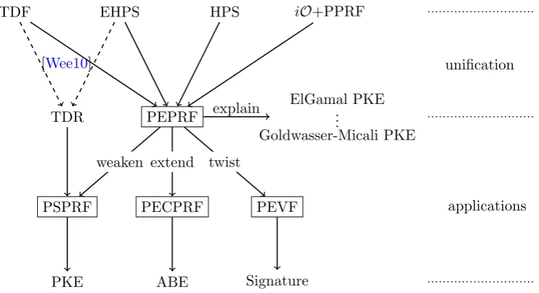
We give positive answers to the above questions. Our main results (summarized in Figure 1) are as follows:
• In Section 3, we introduce the notion of publicly evaluable PRFs (PEPRFs), which is a counterpart of standard PRFs in the public-key setting. In a PEPRF, there is a language
L⊆Xdefined by a hard relationRL, and each secret keyskis associated with a public key
pk. For any x∈L, except via a private evaluation algorithm with sk, one can efficiently evaluate Fsk(x) using pk and a witness w for x ∈ L. We also formalize security notions
for PEPRFs, namely weak pseudorandomness and adaptive weak pseudorandomness.
• In Section4, we demonstrate the power of PEPRFs by showing that they enable the PRF-based private-key encryption to work in the public-key setting, following the KEM-DEM methodology. In sketch, the public/secret key for PEPRF serves as the public/secret key for PKE. To encrypt a messagem, a sender first samples a randomx∈Lwith witnessw, then publicly evaluatesFsk(x) frompk,xandw, and outputs a ciphertext (x, m⊕Fsk(x)).
To decrypt, a receiver simply usessk to computeFsk(x) privately, then recoversm. Such
construction is simple, black-box, and admits a direct proof of security.3 In particular, in Section 3.1we show that the celebrated Goldwasser-Micali PKE and ElGamal PKE can be explained neatly by weak pseudorandom PEPRFs based on the quadratic residuosity assumption and the decisional Diffie-Hellman assumption, respectively.
• In Section 5, Section 6 and Section 7, we show how to construct PEPRFs from trap-door functions (TDFs), hash proof systems (HPSs), and extractable hash proof systems (EHPSs), respectively. This indicates that previous works on TDFs, HPSs and EHPSs im-plicitly constructed PEPRFs. Therefore, PEPRFs are abstraction of the common aspect of HPSs and EHPSs which are not formalized before. Moreover, existing constructions of TDFs, HPS and EHPS imply that PEPRFs can be instantiated from a variety of number-theoretic assumptions. In Section8, we show that recent work [SW14] essentially suggests a way to compile puncturable PRFs to adaptive weak pseudorandom PEPRFs via indis-tinguishability obfuscator. This result reinforces the intuition that in several obfuscation-based constructions the indistinguishability obfuscator is in fact compiling puncturable PRFs into some kind of publicly computable PRFs as an intermediate object.
• In Section9, we introduce the notion of publicly sampleable PRFs (PSPRFs), which is a relaxation of PEPRFs, but nonetheless implies PKE. Of independent interest, we redefine the notion of trapdoor relations (TDRs). We show that injective TDFs imply “one-to-one” TDRs, while the latter further imply PSPRFs. This implication helps us to unify and
3For simplicity, we treat PKE schemes as key encapsulation mechanisms (KEM) in this work. It is well
clarify more PKE schemes based on different paradigms and general assumptions from a conceptual standpoint, and also suggests adaptive PSPRFs as a candidate of the weakest general assumption for CCA-secure PKE.
• In Section10, we introduce an extension of PEPRFs named publicly evaluable constrained PRFs (PECPRFs). An immediate application of PECPRFs is attribute-based encryption. We also present an instantiation of PECPRFs based on an attribute-based encryption scheme from multilinear maps [GGH+13c].
• In Section 11, we propose a twist on PEPRFs named publicly evaluable and verifiable functions (PEVFs), which enjoy an additional property named public verifiability and only require unpredictability rather than weak pseudorandomness. We demonstrate the utility of PEVFs by presenting a simple construction of “hash-and-sign” signatures, both in the random oracle model and the standard model.
TDF EHPS HPS iO+PPRF
PEPRF
ElGamal PKE
Goldwasser-Micali PKE ..
. TDR
unification
applications PSPRF
PKE
PEVF
Signature PECPRF
ABE [Wee10]
explain
twist weaken extend
Figure 1: Summary of main results in this work. The bold lines and rectangles denote our contributions and our new concepts, while the dashed lines denote those from existing works.
1.3 Related Work
CCA-secure PKE from general assumptions or paradigms. Except the effort on con-structing CCA-secure PKE from specific assumptions [HK08,MH14] or from encryption schemes satisfying some weak security notions [NY90,DDN00,BCHK07,CHK10,HLW12,DS13,LT13], it is of great theoretical interest to build CCA-secure PKE from general assumptions and paradigms. Cramer and Shoup [CS02] generalized their CCA-secure PKE construction [CS98] to the notion of hash proof systems (HPSs) and used it as a paradigm to construct CCA-secure PKE from various decisional assumptions. Kurosawa and Desmedt [KD04] and Kiltz et al. [KPSY09] later improved upon the original HPS paradigm. Peikert and Waters [PW08] proposed lossy trapdoor functions (LTDFs) and showed a black-box construction of CCA-secure PKE from them. Rosen and Segev [RS10] introduced correlated-product secure trapdoor func-tions (CP-TDFs) and also showed a construction of CCA-secure PKE from them. Moreover, they showed that CP-TDFs are strictly weaker than LTDFs by giving a black-box separation be-tween them. Kiltz et al. [KMO10] introduced (injective) adaptive trapdoor functions (ATDFs) which are strictly weaker than both LTDFs and CP-TDFs but suffice to imply CCA-secure PKE. Wee [Wee10] introduced the notion of extractable hash proof systems (EHPSs) and used it as a paradigm to construct CCA-secure PKE from various search assumptions. Wee also showed that both EHPS and ATDFs imply (injective) adaptive trapdoor relations (ATDRs), which are sufficient to imply CCA-secure PKE. To the best of our knowledge, the notion of ATDRs is the weakest general assumption that implies CCA-secure PKE.
Constrained PRFs. Very recently, constrained PRFs are studied in three concurrent and independent works, by Kiayias et al. [KPTZ13] under the name ofdelegatable PRFs, by Boneh and Waters [BW13] under the name of constrained PRFs, and by Boyle, Goldwasser, and Ivan [BGI14] under the name offunctional PRFs. In constrained PRFs, the secret key admits a delegation for a family of circuits, and the delegated key for circuit f enable one to compute the PRF value at any pointxsuch thatf(x) = 1. This natural extension turns out to be useful since it has powerful applications outside the scope of standard PRFs, such as identity-based key exchange, and optimal private broadcast encryption.
Witness PRFs. Independently and concurrently of our work, Zhandry [Zha16] introduces the notion ofwitness PRFs (WPRFs), which is similar in concept to PEPRFs. In a nutshell, both WPRFs and PEPRFs are defined with respect to a language and extend standard PRFs with the same extra functionality, i.e., one can publicly evaluate Fsk(x) for x ∈ L with its witness. The main differences between WPRFs and PEPRFs are as follows:
1. In WPRFs the associated relation of the language is required to be polynomially bounded, while in PEPRFs the associated relation of the language is required to be hard.
2. WPRFs require thatFsk(x) is pseudorandom for any adversarially chosenx∈X\L, while
PEPRFs only require thatFsk(x) is pseudorandom for randomly chosenx∈L.
WPRFs are introduced as a weaker primitive to replace indistinguishability obfuscation for several obfuscation-based applications. By utilizing the reduction from any N P language to the subset-sum problem, WPRFs can handle arbitraryN Planguages. However, for applications of WPRFs whose functionalities rely on Fsk(x) forx ∈L, such as public-key encryption,
non-interactive key exchange, and hardcore functions for any one-way function, the underlyingN P
languages have to be at least hard-on-average (i.e., the associated relation is hard). This is because these applications usually need the indistinguishability betweenx←−R Land x←−R X\L
to argue Fsk(x) is computationally pseudorandom for x
2
Preliminaries
2.1 Basic Notations
We review the basic terminology used throughout the paper. For a distribution or a set S, we writes←−R S to denote the operation of samplingsaccording toS or uniformly at random from
S, and use|S|to denote its size. For a setS, we letUS denote the uniform distribution overS.
We letNdenote the positive integers. The natural security parameter throughout the paper
is λ, and all other quantities as well as all algorithms (including the adversary) are implicitly functions of λ. We write poly(λ) to denote an arbitrary polynomial function in λ. We write
negl(λ) to denote an arbitrary negligible function inλ, which vanishes faster than the inverse of any polynomial. We say a probability is overwhelming if it is 1−negl(λ), and said to be noticeable if it is 1/poly(λ). A probabilistic polynomial-time (PPT) algorithm is a randomized algorithm that runs in time poly(λ). If A is a randomized algorithm, we write z ← A(x1, . . . , xn;r) We
will omit r and write z← A(x1, . . . , xn). In addition, we assume an algorithm always outputs
⊥when its input is ⊥.
The statistical distance between two random variables X and Y having a common domain
S is ∆[X, Y] = 12P
s∈S|Pr[X=s]−Pr[Y =s]|. We write≈cas shorthand for computationally
indistinguishable.
2.2 Languages and Relations
Cryptographic hard problems are usually given by a set of instances, which we denote by X. We call a subsetLofX as a language, in which all its elements meet some property. Typically, a language L can be associated with a binary relation RL ⊆ X ×W, i.e., x ∈ L ⇔ ∃w ∈
W s.t. (x, w) ∈ RL. The only restriction is that if (x, w) ∈ RL, then |w| ≤ poly(|x|). We call
w∈W a witness for the membership ofx∈L. We recall some properties of relations as below.
1. Easy to sample a tuple: There exists a PPT algorithm SampRel that on input a public
description ppforRLand fresh random coinsr, outputs a random tuple (x, w)∈RL. We can further decompose SampRel toSampLanand SampWit. The former on input pp and
r outputs x ∈ L, while the latter on input pp and r outputs w ∈ W.4 Hereafter, let R
be the random coins space ofSampRel,SampLan, andSampWit. We require that for any
r∈R, it holds that (SampLan(r),SampWit(r))∈RL.
2. Hard to find a witness: Given x where (x, w) ← SampRel(pp;r), no PPT algorithm can
computew0 such that (x, w0)∈RL with non-negligible probability.
3. Easy to verify a tuple: RLis polynomially-verifiable (i.e., RL∈ P).
We say a relationRL ishard orone-way if it satisfies the first two properties. We say a relation
RL is polynomially bounded if it satisfies the third property. Polynomially bounded relations
define the usualN P language.
Definition 2.1 (Subset membership problem). Let L ⊂ X be a language, and both L and
X\L allow efficiently uniform sampling (let SampYesand SampNo be the sampling algorithms respectively5). We say subset membership problem w.r.t. (X, L) is hard if:
UX\L≈cUL
4When the context is clear, we usually omitppfrom the input ofSampRel. 5
2.3 Pseudorandom Functions
We first recap the definition of PRFs in order to compare them with PEPRFs more clearly.
Definition 2.2 (PRFs [GGM86]). A family of PRFs consists of three polynomial-time algo-rithms as follows:
• Setup(1λ): on input 1λ, output public parameters pp = (F, SK, X, Y) (the sets SK, X, and Y may be parameterized by λ), where F : SK×X → Y can be viewed as a keyed function indexed bySK, namely F={Fsk}sk∈SK.
• KeyGen(pp): on inputpp, output a secret keysk∈SK.
• PrivEval(sk, x): on input sk and x∈X, output y∈Y.
Correctness: For any λ∈N, any pp ←Setup(1λ), any sk ←KeyGen(pp) and any x∈X, we have Fsk(x) =PrivEval(sk, x).
Security: The standard security requirement for PRFs is pseudorandomness. Let A be an adversary against PRFs and define its advantage as:
AdvA(λ) = Pr
b=b0 :
pp←Setup(1λ);
sk←KeyGen(pp);
b← {0,1};
b0 ← AOror(b,·)(pp);
−1
2,
whereOror(0, x) =Fsk(x),Oror(1, x) =H(x) (hereHis chosen uniformly at random from all the
functions from X to Y6). Note that A can adaptively access the oracle Oror(b,·) polynomial
many times. We say that PRFs are pseudorandom if for any PPT adversary its advantage functionAdvA(λ) is negligible inλ. We refer to such security as full PRF security.
Sometimes the full PRF security is not needed and it is sufficient if the function cannot be distinguished from a uniform random one when challenged on random inputs. The formalization of such relaxed requirement is weak pseudorandomness (weak PRF security), which is defined the same way as the full PRF security except that the inputs of oracleOror(b,·) are uniformly
chosen fromX by the challenger instead of adversarially chosen by A. PRFs that satisfy weak pseudorandomness are referred to as weak PRFs.
2.4 Secret-Coin vs. Public-Coin Weak PRFs
In the original syntax of PRFs, the input-sampling algorithm is not implicitly given. Note that in the weak PRF security experiment challenge points are sampled by the challenger, thus it is convenient to explicitly introduce an input-sampling algorithm to obtain more refined security notions for weak PRFs. Hereafter, let SampDom be an algorithm that takes as input random coinsr and outputs an element x∈X. Without loss of generality, we assume the distribution of x induced by SampDom(r) conditioned onr ←−R R is statistically close tox ←−R X. Hence, in the weak PRF security experiment, the challenger can sample elements uniformly at random from X by running SampDom with random coins r ←−R R. Depending on whether the random coinsrcan be made public, weak PRFs are further divided into secret-coin and public-coin weak PRFs [PS08]. Secret-coin weak PRFs require weak pseudorandomness holds if the random coins are kept secret, whereas public-coin weak PRFs requires weak pseudorandomness holds even the random coins are made public. Clearly, whether a weak PRF is public-coin or just secret-coin depends on the input-sampling algorithm.
6
To efficiently simulate access to a uniformly random functionHfromX toY, one may think of a process in which the adversary’s queries toOror(1,·) are “lazily” answered with independently and randomly chosen elements
3
Publicly Evaluable PRFs
Here we define PEPRFs. We begin with the syntax and then define the security.
Definition 3.1 (Publicly Evaluable PRFs). A family of PEPRFs consists of four polynomial-time algorithms as below:
• Setup(1λ): on input 1λ, output public parametersppwhich includes (F, P K, SK, X, L, W, Y), whereF:SK×X →Y ∪ ⊥ could be viewed as a keyed function indexed bySK,L⊆X
is a language defined by some hard relationRL, and W is the set of associated witnesses. We assume RL is efficiently sampleable, that is, there exists a PPT algorithm SampRel
which on input random coinsr, output a random tuple (x, w)∈RL.
• KeyGen(pp): on inputpp, output a secret keysk and an associated public keypk.7
• PrivEval(sk, x): on input sk and x∈X, output y∈Y ∪ ⊥.
• PubEval(pk, x, w): on input pkand x∈L together with a witness w∈W, output y∈Y.
Correctness: For any λ∈N, any pp←Setup(1λ) and any (pk, sk)←KeyGen(pp), we have:
∀x∈X: Fsk(x) =PrivEval(sk, x)
∀x∈L with a witnessw: Fsk(x) =PubEval(pk, x, w)
Security: LetA be an adversary against PEPRFs and define its advantage as:
AdvA(λ) = Pr
b=b0:
pp←Setup(1λ);
(pk, sk)←KeyGen(pp);
{r∗i ←−R R,(x∗i, w∗i)←SampRel(ri∗)}pi=1(λ);
b← {0,1};
b0 ← AOeval(·)(pp, pk,{x∗
i,Oror(b, x∗i)} p(λ)
i=1);
−1
2,
where p(λ) is any polynomial, Oeval(x) = Fsk(x), Oror(0, x) = Fsk(x), Oror(1, x) = H(x), and
A is not allowed to query Oeval(·) with any x∗i. We say that PEPRFs are adaptive weak pseudorandom if for any PPT adversary A its advantage function AdvA(λ) is negligible in λ.8
The adaptive weak pseudorandomness captures the security against active adversaries, who are given adaptive access to the oracle Oeval(·). We also consider weak pseudorandomness which captures the security against static adversaries, who is not given access to oracle Oeval(·).
On the basis of previous works [BK03,BC10,HLAWW13], one can also define more advanced security notions such as security against related-key attacks and security against key-leakage attacks for PEPRFs.
Remark 3.1. Different from standard PRFs, PEPRFs require the existence of a languageL⊆X
as well as a public evaluation algorithm. Due to this strengthening on functionality, we cannot hope to achieve full PRF security, and hence settling for weak PRF security is a natural choice.9 Note that the weak PRF security implicitly requires that the associated relation RL is hard.
7
In a standard PRF, it is also harmless to explicitly introduce a public key, which includes the information related to secret key that can be made public. For example, in the Naor-Reingold PRF [NR04] based on the DDH assumption: F~a(x) = (ga0)
Q
xi=1ai, where~a= (a
0, a1, . . . , an)∈Znp is the secret key,gai for 1≤i≤ncan be safely published as the public key. If no information can be made public, one can always assumepk={⊥}.
8The readers should not be confused with adaptive PRFs [BH12], where “adaptive” means that instead of
deciding the queries in advance, an adversary can adaptively make queries toOror(b,·) based on previous queries.
9In the full PRF security experiment the inputs ofO
ror(b,·) are chosen by an adversary, thus it may know the
Remark 3.2. In some scenarios, it is more convenient to work with a definition that slightly restricts an adversary’s power, but is equivalent to Definition 3.1. That is, the query times
p(λ) by an adversary is fixed to 1. Due to the existence of oracle Oeval(·), a standard hybrid
argument can show that PEPRFs secure under this restricted definition are also secure under Definition3.1. In the remainder of this paper, we will work with this restricted definition.
A possible relaxation. To be completely precise, it is not necessary to require the distribution of xinduced by SampRel(r) conditioned on r ←−R R is identical or statistically close to uniform. Instead, it could be some other prescribed distributionχ. In this case, weak pseudorandomness extends naturally toχ-weak pseudorandomness.
A useful generalization. In some scenarios, it is more convenient to work with a more gener-alized notion in which we consider a collection of languages {Lpk}pk∈P K indexed by the public
key rather than a fixed languageL. Correspondingly, the sampling algorithmSampReltakes pk
as an extra input to sample a random tuple (x, w)∈RLpk. We refer to such generalized notion
as PEPRFs for public-key dependent languages, and we will work with it when constructing
adaptive PEPRFs from hash proof systems.
3.1 Two Simple PEPRFs from Number-Theoretic Assumptions
In what follows, we present two illustrative constructions of PEPRFs from the quadratic residu-osity (QR) assumption (c.f. AppendixA.6) and the decisional Diffie-Hellman (DDH) assumption (c.f. AppendixA.7), respectively.
Construction 3.1. We build PEPRFs from the QR assumption as follows:
• Setup(1λ): run (N, p, q) ← GenModulus(1λ), set X = Z∗N, Y = {0,1}, P K = {N} ×
QN R+1N ,SK={p} × {q},W =ZN∗ ,F:SK×X→Y will be defined later;Lbe the set of
elements in Z∗N having Jacobi symbol +1. Letz be an element inQN R
+1
N , we can define
L = {x : ∃w ∈ W s.t.x = w2 modN ∨x = zw2 modN}, the corresponding sampling
algorithm SampRel on input 1λ, public key (N, z), and random coins r, picks w ←−R Zp, computes eitherx=w2 modN orx=zw2 modN, then outputs (x, w).
• KeyGen(pp): pickz←−R QN R+1N , output pk= (N, z) andsk= (p, q).
• PrivEval(sk, x): output 1 if Jacobip(x) = Jacobiq(x) = 1 and 0 otherwise. This algorithm
defines F:SK×X→Y.
• PubEval(pk, x, w): output 1 if x=w2modN and 0 ifx=zw2 modN.
It is easy to verify that the above PEPRFs are weak pseudorandom based on the QR assump-tion. Looking ahead, applying the construction shown in Section 4 to the PEPRFs yields the Goldwasser-Micali PKE [GM84].
Construction 3.2. We build PEPRFs from the DDH assumption as follows:
• Setup(1λ): run (G, p, g) ← GroupGen(1λ), set X =Y = P K =L = G, SK = W =Zp, F:SK×X →Y is defined asFsk(x) =xsk; we can define L={x:∃w∈W s.t.x=gw};
the corresponding sampling algorithm SampRel on input λ and random coins r, picks
w←−R Zp, computes x=gw, then outputs (x, w).
• KeyGen(pp): picksk ←−R Zp, computepk=gsk, output (pk, sk).
• PrivEval(sk, x): output xsk.
• PubEval(pk, x, w): output pkw.
3.2 Relation to Secret-Coin and Public-Coin Weak PRFs
It is easy to see that PEPRFs naturally imply secret-coin weak PRFs by letting the input-sampling algorithm simply run (x, w)←SampRel(r) and only outputx. In fact, PEPRFs can be viewed as a special case of secret-coin weak PRFs, where the weak PRF security completely breaks down if the random coins used to sample the challenge inputs are revealed. Also, ev-ery public-coin weak PRF is clearly a secret-coin weak PRF. We depict the relations among secret-coin, public-coin, and publicly evaluable PRFs in Figure2. On one hand, Pietrzak and Sj¨odin [PS08] demonstrated that the existence of a secret-coin weak PRF which is not also a public-coin weak PRF implies the existence of two pass key-agreement and thus two pass public-key encryption. This result indicates that PEPRFs must be very artificial in Minicrypt. On the other hand, as we will see shortly, PEPRFs admit a black-box construction of PKE, which implies that PEPRFs are strictly stronger than PRFs (in a black-box sense).
Interestingly, secret-coin PRFs can be intuitively constructed from PEPRFs and public-coin PRFs. Suppose {Gsk1 :X1 → Y1}sk1∈SK1 is a public-coin PRF and {Hsk2 :X2 → Y2}sk2∈SK2
is a PEPRF, then {Fsk1,sk2(x1, x2) := (Gsk1(x1),Hsk2(x2))}constitutes a secret-coin PRF from X1×X2 toY1×Y2 indexed by SK1×SK2.
weak PRFs
publicly evaluable PRFs secret-coin weak
PRFs
public-coin weak PRFs
Figure 2: Relations among secret-coin, public-coin, and publicly evaluable PRFs.
4
KEM from Publicly Evaluable PRFs
In this section, we present a simple and black-box construction of KEM from PEPRFs. For compactness, we refer the reader to AppendixA.1for the definition and security notion of KEM.
• Setup(1λ): run PEPRF.Setup(1λ) to generatepp as public parameters.
• KeyGen(pp): run PEPRF.KeyGen(pp) to generate (pk, sk).
• Encaps(pk;r): run SampRel(r) to generate a random tuple (x, w) ∈ RL, set x as the ciphertext cand compute PEPRF.PubEval(pk, x, w) as the DEM key k, output (c, k).
• Decaps(sk, c): output PEPRF.PrivEval(sk, c).
Correctness of the above KEM construction follows immediately from correctness of PEPRFs. For security, we have the following results:
Theorem 4.1. The KEM is CPA-secure (resp. CCA-secure) if the underlying PEPRFs are weak pseudorandom (resp. adaptive weak pseudorandom).
Proof. The proof is straightforward, which transforms an adversary A against IND-CPA
pseudorandomness (resp. adaptive weak pseudorandomness) of PEPRFs. Here, we only prove the IND-CCA case and the IND-CPA case immediately follows.
B simulatesA’s challenger in the standard IND-CCA experiment.
• Setup and challenge: B receives (pp, pk, x∗, y∗b) from its own challenger, where pp ←
PEPRF.Setup(1λ), (pk, sk) ← PEPRF.KeyGen(pp), (x∗, w∗) ← SampRel(r∗) for some random coins r∗, and yb∗ is Fsk(x∗) if b= 0 or randomly chosen from Y ifb = 1. B sets
c∗ =x∗,k∗b =yb∗, and sends (pp, pk, c∗, kb∗) to Aas the challenge.
• Decapsulation queries: on decapsulation query hxi where x 6=x∗, B submits evaluation query on point x to its own challenger and forwards the reply toA.
• Guess: Aoutputs its guess b0 forband B forwardsb0 to its own challenger.
Clearly, B simulates the IND-CCA experiment perfectly. Therefore, B can break the adaptive weak pseudorandomness of PEPRFs with advantage at least AdvCCAA (λ). Assuming the
adap-tive weak pseudorandomness of the underlying PEPRFs, AdvCCAA (λ) is negligible in λ. This
concludes the proof.
The above results also hold if the underlying PEPRFs are (adaptive)χ-weak pseudorandom.
5
Connection to Trapdoor Functions
Trapdoor functions (TDFs) are a fundamental primitive introduced by Diffie and Hellman [DH76]. In the following, we recall the syntax and security notions of TDFs and then show how to con-struct PEPRFs from them.
Definition 5.1(Trapdoor Functions). A family of trapdoor functions is given by four polynomial-time algorithms as below.
• Setup(1λ): on input 1λ, output public parameterspp= (TDF, P K, SK, S, U), whereTDF:
P K×S →U can be viewed as a keyed function indexed byP K. We assume the domainS
is efficiently sampleable, that is, there exists a PPT algorithmSampDom, which on input random coinsr←−R R, output a random element s∈S.
• KeyGen(pp): on input pp, output a public key pk (serve as a key for evaluation) and a corresponding secret keysk (serve as a trapdoor for inversion).
• Eval(pk, s): on inputpk and s∈S, output u←TDFpk(s).
• TdInv(sk, u): on inputsk andu∈U, outputs∈Sor a distinguished symbol⊥indicating
u does not have pre-image.
Correctness: For any λ ∈ N, any pp ← Setup(1λ), any (pk, sk) ← KeyGen(pp) and any
s=Eval(pk, u), we haveEval(pk,TdInv(sk, s)) =s.
(Adaptive) One-wayness: Let Abe an inverter against TDFs and define its advantage as:
AdvA(λ) = Pr
s∈TDF−pk1(u∗) :
pp←Setup(1λ);
(pk, sk)←KeyGen(pp);
u∗←Eval(pk, s∗), s∗ ←SampDom(r∗);
s← AOinv(·)(pp, pk, u∗)
,
where Oinv(u) = TdInv(sk, u), andA is not allowed to queryOinv(·) for the challenge u∗. We
Definition 5.2 (Hardcore Functions). A polynomial-time algorithm hc:S → Y is said to be a hardcore function of a family of efficiently computable functions F:P K×S → U if for any PPT algorithmA, the following two distributions are computationally indistinguishable:
(pp, pk,Fpk(s),hc(s))≈c(pp, pk,Fpk(s), y)
wherepp←Setup(1λ),pk←KeyGen(pp),s←SampDom(r),y←R−Y.
Corollary 1. Let F be a family of efficiently computable injective functions. F is one-way if
and only if F has a hardcore function hc.
5.1 Construction from (Adaptive) Injective TDFs
From (adaptive) injective TDFs, we construct PEPRFs as follows:
• Setup(1λ): on input 1λ, run TDF.Setup(λ) to generate pp = (TDF, P K, SK, S, U) for TDFs, and let hc : S → Y be a corresponding hardcore function; then create public parameters pp = (F, P K, SK, X, L, W, Y) for PEPRFs as follows: set P K and SK the same as that of TDFs, set Y the same as that of the hardcore function, set X = U,
W =S,Fwill be defined latter. The algorithm TDF.Evalinduces a collection of languages
L = {Lpk}pk∈P K over X where each Lpk = {x : ∃w ∈ W s.t. x = TDF.Eval(pk, w)}.
The sampling algorithm SampRel on input r, runs s ← SampDom(r), computes u ←
TDF.Eval(pk, s), and then outputs x =u and w=s. We assume the public parameters
pp of TDFs and PEPRFs contain essentially the same information.
• KeyGen(pp): on inputpp, output (pk, sk)←TDF.KeyGen(pp).
• PrivEval(sk, x): on inputskandx∈X, outputy ←hc(TDF.TdInv(sk, x)). This algorithm defines F:SK×X→Y ∪ ⊥.
• PubEval(pk, x, w): on inputpkandx∈Lpk together with a witnessw, outputy←hc(w).
The correctness of the above construction follows from the correctness and injectivity of TDFs. For the security, we have the following theorem.
Theorem 5.1. PEPRFs are weak pseudorandom (resp. adaptive weak pseudorandom) if the underlying TDFs are one-way (resp. adaptive one-way).
Proof. The proof is straightforward, which transforms an adversary A against weak
pseudo-randomness (resp. adaptive weak pseudopseudo-randomness) of PEPRFs to an adversary B against pseudorandomness (resp. adaptive pseudorandomness) of hc, and thus contradicts to the as-sumed one-wayness (resp. adaptive one-wayness) of TDFs. Here, we only prove the adaptive weak pseudorandomness case and the weak pseudorandomness case immediately follows.
B simulatesA’s challenger in the adaptive weak pseudorandomness experiment for PEPRFs.
• Setup and challenge: B receives (pp, pk, u∗, yb∗) from its own challenger, where pp ←
TDF.Setup(1λ), (pk, sk) ← TDF.KeyGen(pp), u∗ ← TDF.Eval(pk, s∗) for some s∗ ←−R S, and yb∗ is hc(s∗) if b = 0 or randomly chosen from Y if b = 1. B sets x∗ = u∗, sends (pp, pk, x∗, yb∗) to Aas the challenge.
• Evaluation queries: on evaluation query x6=x∗,B queries the inversion oracle at point x
and gets the response s,B then responds with hc(s).
• Guess: Aoutputs its guess b0 forband B forwardsb0 to its own challenger.
Clearly, B simulates the adaptive weak pseudorandomness experiment perfectly. Therefore, B
can break pseudorandomness ofhcwith advantage at leastAdvA(λ). Assuming the one-wayness
6
Connection to Hash Proof Systems
Hash proof systems are introduced by Cramer and Shoup [CS02] as a paradigm of constructing PKE from a category of decisional problems, named subset membership problems. As a warm up, we first recall the notion of HPS and then show how to construct PEPRFs from them.
Definition 6.1 (Hash Proof System). An HPS consists of the following algorithms:
• Setup(1λ): on input 1λ, output public parameters pp which includes an HPS instance (Λ, SK, P K, X, L, W,Π, α), where Λ : SK ×X → Π can be viewed as a keyed function indexed bySK,Lis a language defined overX,W is the associated witness set, andα is a projection fromSK toP K.
• KeyGen(pp): on inputpp, picksk←−R SK, computepk←α(sk), output (pk, sk).
• PrivEval(sk, x): on input sk and x, output π= Λsk(x).
• PubEval(pk, x, w): on input pkand x∈L together with a witness w, output π= Λsk(x).
Following [CS02,KPSY09] we introduce the following notions and properties for Λ onX\L.
Collision probability. The collision probability of Λ is defined as:
δ= max
x,x∗∈X\L,x6=x∗(Prsk[Λsk(x) = Λsk(x ∗
)]).
Universal1. Λ is -universal1 if for all x∈X\L,
∆[(pk,Λsk(x)),(pk, π)]≤,
where (pk, sk)←KeyGen(λ) and π ←−R Π.
[CS02] introduced a relaxation of universal1 property, named smoothness, which only
re-quires the universal1 property holds in the average case.
Smoothness. Λ is-smooth if forx←−R X\L,
∆[(pk,Λsk(x)),(pk, π)]≤,
where (pk, sk)←KeyGen(λ) and π ←−R Π.
[CS02] also introduced a strengthening of universal1 property, named universal2 property.
Universal2. Λ is -universal2 if for all x, x∗∈X\Lwith x6=x∗,
∆[(pk,Λsk(x∗),Λsk(x)),(pk,Λsk(x∗), π)]≤
where (pk, sk)←KeyGen(λ) and π ←−R Π.
Kiltz, Pietrzak, Stam, and Yung [KPSY09] (henceforth KPSY) provides a generic transform from universal1to universal2HPS. Given a HPS with hash Λ :SK×X→Π regarding projection
α:SK →P Kand a family of functionsH={h: Π→ {0,1}`}, we can define its hashed variant
HPSHwith hash ΛH:SKH×X→ {0,1}` regardingαH:SKH→P KH whereP KH=P K×H,
SKH = SK×H, ΛH((sk,h), x) =h(Λ(sk, x)) and αH(sk,h) = (α(sk),h). Note that X and L
are the same for HPS and HPSH.
Theorem 6.1 ([KPSY09]). Assume Λ is 1-universal1 with collision probability δ ≤ 1/2 and
H={h: Π→ {0,1}`} (where`≥6) is a family of 4-wise independent hash functions, then ΛH
is 2-universal2 for:
2 = 2`−
λ−1
6.1 Construction from Smooth HPS
From smooth HPS, we construct weak pseudorandom PEPRFs as follows:
• Setup(1λ): on input 1λ, run HPS.Setup(1λ) to generate a smooth HPS instance pp = (Λ, P K, SK, X, L, W,Π, α), then create pp= (F, P K, SK, X, L, W, Y) for PEPRFs as fol-lows: setP K,SK,X,L, andW the same as that of HPS, setF= Λ,Y = Π. We assume the public parameterspp of HPS and PEPRFs contain essentially the same information.
• KeyGen(pp): on inputpp, output (pk, sk)←HPS.KeyGen(pp).
• PrivEval(sk, x): on input sk and x∈X, output y←HPS.PrivEval(sk, x).
• PubEval(pk, x, w): on input pk and x ∈ L together with a witness w∈ W for x, output
y←HPS.PubEval(pk, x, w).
We have the following theorem about the above construction.
Theorem 6.2. If the underlying subset membership problem is hard, then the PEPRFs from the smooth HPSs are weak pseudorandom.
Proof. The proof is similar to [CS02]. To establish weak pseudorandomness based on the
hard-ness of underlying subset membership problem, we proceed via a sequence of games. Let Si be
the event that Aoutputs the right guess in Game i.
Game 0(standard weak pseudorandomness experiment for PEPRFs)
• Setup and challenge: CHruns HPS.Setup(1λ) to build public parameters ppfor PEPRFs, and runs HPS.KeyGen(pp) to generate a key pair (pk, sk). CH then runs (x∗, w∗) ←
SampRel(r∗) for r∗ ←−R R, computesπ∗ ←Λsk(x∗) via HPS.PubEval(pk, x∗, w∗), sets y∗0 =
π∗, and picksy1∗←R−Y. Finally,CHpicksb←R− {0,1}, and sends (pp, pk, x∗, yb∗) toAas the challenge.
• Guess: Aoutputs its guess b0 and wins ifb0 =b.
According to the definition ofA, we have:
AdvA(λ) =|Pr[S0]−1/2| (1)
Game 1: same as Game 0 except that CH computes π∗ ← Λsk(x∗) via HPS.PrivEval(sk, x∗).
According to the functionality ofPrivEvalandPubEval, this change is perfectly hidden from the adversary. Thus, we have:
Pr[S1] = Pr[S0] (2)
Game 2: same as Game 1 except thatCHsamplesx∗via algorithmSampNoinstead ofSampRel. The sampling indistinguishability (based on the hardness of the subset membership problem) ensures that:
|Pr[S2]−Pr[S1]| ≤negl(λ) (3)
Game 3: same as Game 2 except thatCH setsy0∗ asπ0, whereπ0 ←−R Π. It now follows directly from the -smooth property of HPS that:
|Pr[S3]−Pr[S2]| ≤ (4)
It is evident that in Game 3A’s outputb0 is independent of the hidden bitb, therefore:
Pr[S3] = 1/2 (5)
6.2 Construction from Smooth and Universal2 HPS
From a smooth HPS and an universal2 HPS for the same language ˜L ⊂ X˜, we can construct
adaptive weak pseudorandom PEPRFs as follows:
• Setup(1λ): on input 1λ, run HPS1.Setup(1λ) to generate a smooth HPS instance pp1 =
(Λ1, P K1, SK1, ˜X, ˜L, ˜W, Π1, α1), run HPS2.Setup(1λ) to generate an universal2 HPS
instance pp2 = (Λ2, P K2, SK2, ˜X, ˜L, ˜W, Π2, α2), then build public parameters pp =
(F, P K, SK, X, L, W, Y) for PEPRFs from pp1 and pp2 as follows, sets X = ˜X ×Π2,
Y = Π1∪ ⊥,P K=P K1×P K2,SK =SK1×SK2,W = ˜W,Fwill be defined later. The
algorithm HPS2.PubEvalinduces a collection of languagesL={Lpk}pk∈P K overX= ˜X×
Π2, where each Lpk ={x= (˜x, π2) :∃w∈W s.t. ˜x∈L˜∧π2 = HPS2.PubEval(pk2,x, w˜ )}.
The corresponding sampling algorithm L.SampRel on input pk = (pk1, pk2) and random
coins r, runs (˜x,w˜) ← L.˜SampRel(r), computesπ2 ← HPS2.PubEval(pk2,x,˜ w˜), sets x =
(˜x, π2), w = ˜w, outputs (x, w). We assume the two HPSs share a common sampling
algorithm andpp=pp1∪pp2.
• KeyGen(pp): on input pp =pp1∪pp2, run HPS1.KeyGen(pp1) and HPS2.KeyGen(pp2) to
get (pk1, sk1) and (pk2, sk2) respectively, output pk= (pk1, pk2),sk= (sk1, sk2).
• PrivEval(sk, x): on inputsk= (sk1, sk2) andx= (˜x, π2), outputy←HPS1.PrivEval(sk1,x˜)
if π2 = HPS2.PrivEval(sk2,x˜) and ⊥ otherwise. This algorithm defines F : SK ×X →
Y ∪ ⊥.
• PubEval(pk, x, w): on input pk = (pk1, pk2) and an element x = (˜x, π2) ∈ Lpk together
with a witnessw, output y←HPS1.PubEval(pk1,x, w˜ ).
We have the following theorem about the above construction.
Theorem 6.3. If the underlying subset membership problem is hard, then the PEPRFs from
the smooth and universal2 HPSs are adaptive weak pseudorandom.
Proof. The proof is similar to [CS02]. To base adaptive weak pseudorandomness on the hardness
of underlying subset membership problem, we proceed via a sequence of games. Let Si be the
event that Aoutputs the right guess in Gamei.
Game 0(standard adaptive weak pseudorandomness experiment for PEPRFs)
• Setup and challenge: CH prepares the challenge via the following steps:
1. run HPS1.Setup(1λ) and HPS2.Setup(1λ) to generatepp1 and pp2 for a smooth HPS
instance and an universal2HPS instance respectively, then build public parameterspp
for PEPRFs frompp1andpp2; run (pk1, sk1)←HPS1.KeyGen(pp1) and (pk2, sk2)←
HPS2.KeyGen(pp2), set pk= (pk1, pk2) and sk= (sk1, sk2).
2. sample (˜x∗,w˜∗) ← L.˜ SampRel(r∗) with fresh random coins r∗ ←−R R, compute π∗2 = Λ2sk
2(˜x
∗) via HPS
2.PubEval(pk2,x˜∗,w˜∗), set x∗ = (˜x∗, π2∗); compute π1∗ = Λ1sk1(˜x ∗)
via HPS1.PubEval(pk1,x˜∗,w˜∗), set y0∗ = π∗1, sample y1∗
R
←− Y, pick b ←− {R 0,1}, and send (pp, pk, x∗, y∗b) to A as the challenge.
• Evaluation query: on evaluation query at point x 6= x∗, CH responds normally with
sk = (sk1, sk2). More precisely, CH parses x as (˜x, π2), then responds with Λ1sk1(˜x) if
Λ2sk
2(˜x) =π2 and⊥ otherwise.
• Guess: Aoutputs its guess b0 and wins ifb0 =b.
According to the definition ofA, we have:
Game 1: same as Game 0 except thatCH computes π2∗= Λ2sk
2(˜x
∗) via HPS
2.PrivEval(sk2,x˜∗)
and computes π∗1 = Λ1
sk1(˜x
∗) via HPS
1.PrivEval(sk2,x˜∗). According to the functionality of
PrivEvaland PubEval, this change is perfectly hidden from A. Thus, we have:
Pr[S1] = Pr[S0] (7)
Game 2: same as Game 1 except that CH samples ˜x∗ via SampNo instead of SampRel. The sampling indistinguishability (based on the subset membership assumption) ensures that:
|Pr[S2]−Pr[S1]| ≤negl(λ) (8)
Game 3: same as Game 2 except that when answering evaluation querieshxiwherex= (˜x, π2),
CH returns ⊥ if ˜x /∈L˜ even when Λ2
sk2(˜x) = π2. For the ease of analysis, we denote by E the
event that A submits an evaluation query x = (˜x, π2) such that ˜x /∈ L but Λ2sk2(˜x) = π2.
According to the universal2 property of HPS2, we have Pr[E]≤Q, where Q is the maximum
number of evaluation queries thatA may make. Sinceis negligible in λ, we have:
|Pr[S3]−Pr[S2]| ≤Pr[E]≤negl(λ)
Game 4: same as Game 3 except thatCHsetsy∗0 asπ10, whereπ10 ←−R Π1. Now, let us condition
on a fixed value ofpk2,b, andA’s random coins. In this conditional probability space, since the
action of Λ1sk
1 on ˜Lis determined by pk1, and all evaluation queries x= (˜x, π2) with ˜x∈
˜
Lare responded with ⊥, it follows that A’s view in Game 3 is completely determined as a function of ˜x∗, pk1, and π1∗, while A’s view in Game 4 is determined as the same function of ˜x∗, pk1,
and π10. Moreover, by independence, the joint distributions of (˜x∗, pk1, π1∗) and (˜x∗, pk1, π01) do
not change in passing from the original probability space to the conditional probability space. It now follows directly from the-smooth property of Λ1, we have:
|Pr[S4]−Pr[S3]| ≤
It is evident that in Game 4A’s outputb0 is independent of the hidden bitb. Therefore,
Pr[S4] = 1/2
Putting all these above, the theorem immediately follows.
Remark 6.1. To ensure the adaptive weak pseudorandomness of the above construction, we can
weaken universal2 property to weak universal2 property, which requires the former property
holds when x∗ ←−R X\L. This is because adaptive weak pseudorandomness only stipulates pseudorandomness holds on the average case.
6.3 Construction from Universal1 HPS
From an universal1 HPS, we can construct adaptive weak pseudorandom PEPRFs as follows:
• Setup(1λ): on input 1λ, run HPS.Setup(1λ) to generatepp
1 for an universal1 HPS instance
(Λ, P K˜ , SK˜ , ˜X, ˜L, ˜W, Π, α), then apply the KPSY-transform [KPSY09] to obtain an universal2 HPSH, whereHis a family of 4-wise independent hash functions from Π to ΠH;
then build public parameters pp = (F, P K, SK, X, L, W, Y) for PEPRFs from pp1 and H
as follows, whereX = ˜X×ΠH,Y = Π∪ ⊥,P K = ˜P K×P K˜ ×H,SK = ˜SK×SK˜ ×H,
W = ˜W, F will be defined later. The algorithm HPS.PubEval defines a collection of languages L = {Lpk}pk∈P K over X = ˜X ×ΠH where each Lpk = {x = (˜x, πh) : ˜x ∈
˜
L∧πh = h(HPS.PubEval( ˜pk2,x,˜ w˜))}. It is easy to see that a witness ˜w for ˜x ∈ L˜ is also a witness for x = (˜x, πh) ∈ Lpk. The corresponding sampling algorithm on input
pk = ( ˜pk1,pk˜2,h) and random coins r, samples (˜x,w˜) ← L.˜ SampRel(r), computes πh ←
• KeyGen(pp): on input pp = (pp1,H), run HPS.KeyGen(pp1) twice independently to get
( ˜pk1,sk˜1) and ( ˜pk2,sk˜2), pick h
R
←− H, set pk = ( ˜pk1,pk˜2,h), sk = ( ˜sk1,sk˜2,h), output
(pk, sk).
• PrivEval(sk, x): on inputsk= ( ˜sk1,sk˜2,h) andx= (˜x, πh), outputy←HPS.PrivEval( ˜sk1,x˜)
ifπh =h(HPS.PrivEval( ˜sk2,x˜)) and ⊥ otherwise. This algorithm definesF :SK×X →
Y ∪ ⊥.
• PubEval(pk, x, w): on inputpk = ( ˜pk1,pk˜2,h) and an element x= (˜x, πh)∈Lpk together
with a witnessw, output y←HPS.PubEval( ˜pk1,x, w˜ ).
In the above construction, we implicitly build HPSH, which is universal2 according to
Theo-rem 6.1. We have the following theorem about the above construction.
Theorem 6.4. If the underlying subset membership problem is hard, then the PEPRFs from
the universal1 HPSs are adaptive weak pseudorandom.
Proof. The proof is similar as that in Section6.2. To base adaptive weak pseudorandomness on
the universal1 property of Λ and the subset membership problem assumption, we proceed via
a sequence of games. LetSi be the event thatAoutputs the right guess in Gamei.
Game 0(standard adaptive weak pseudorandomness game)
• Setup and challenge: CH prepares the challenge via the following steps:
1. run HPS.Setup(1λ) to generatepp1for an universal1HPS instance and choose a family
of 4-wise independent hash functionsHfrom Π to ΠH, then build public parameters
ppfor PEPRFs fromppandH; runs HPS.KeyGen(pp) twice independently to generate ( ˜pk1,sk˜1) and ( ˜pk2,sk˜2), pick h
R
←−H, setspk= ( ˜pk1,pk˜2,h) and sk= ( ˜sk1,sk˜2,h).
2. sample (˜x∗,w˜∗) ←L.˜ SampRel(r∗) with fresh random coinsr∗ ←−R R, compute πh∗ =
h(Λsk˜2(˜x∗)) via h(HPS.PubEval( ˜pk2,x˜∗,w˜∗)), set x∗ = (˜x∗, πh
∗
); computes π∗ = Λsk˜1(˜x∗) via HPS.PubEval( ˜pk1,x˜∗,w˜∗), set y∗0 = π∗, pick y1∗
R
←− Y, pick b ←− {R 0,1}, and send (pp, pk, x∗, yb∗) to A as the challenge.
• Evaluation query: on evaluation queries at point x 6= x∗, CH responds normally with
sk = ( ˜sk1,sk˜2,h). More precisely, CH parses x as (˜x, πh), then responds with Λsk˜1(˜x) if
h(Λsk˜2(˜x)) =πh and ⊥otherwise.
• Guess: Aoutputs its guess b0 and wins ifb0 =b.
According to the definition ofA, we have:
AdvA(λ) =|Pr[S0]−1/2| (9)
Game 1: same as Game 0 exceptCHcomputesπh∗ =h(Λsk˜2(˜x∗)) viah(HPS.PrivEval( ˜sk2,x˜∗))
and computes y0∗ = Λsk˜1(˜x∗) via HPS.PrivEval( ˜sk1,x˜∗). According to the functionality of
PrivEvaland PubEval, this change is perfectly hidden from A. Thus, we have:
Pr[S1] = Pr[S0] (10)
Game 2: same as Game 1 except that CH samples ˜x∗ via SampNo instead of SampRel. The sampling indistinguishability (based on the subset membership assumption) ensures that:
Game 3: same as Game 2 except that when answering evaluation querieshxiwherex= (˜x, πh),
CH returns ⊥ when ˜x /∈L˜ even h(Λsk˜2(˜x)) =πh. For the ease of analysis, letE be the event
thatAsubmits an evaluation queryx= (˜x, πh) such that ˜x /∈L˜buth(Λsk˜2(˜x)) =πh. According
to the universal2 property of ΛH, we have Pr[E] ≤ Q, where Q is the maximum number of
evaluation queries thatA may make. Sinceis negligible inλ, we have:
|Pr[S3]−Pr[S2]| ≤Pr[E]≤negl(λ)
Game 4: same as Game 3 except that CH setsy∗0 asπ0, where π0 ←−R Π. The rest reasoning is similar as that presented in Section6.2. It now follows directly from the1-universal1 property
of Λ, we have:
|Pr[S4]−Pr[S3]| ≤1
It is evident that in Game 4A’s outputb0 is independent of the hidden bitb. Therefore,
Pr[S4] = 1/2
Putting all these above, the theorem immediately follows.
Remark 6.2. Construction6.1is straightforward, while the construction6.2and construction6.3
are more technically involved. The basic idea underlying the latter two constructions are similar as the CCA-secure PKE from smooth plus universal2 HPSs [CS02]. That is, using a “weak”
HPS to generate a random DEM key, while using a “strong” HPS to eliminate “dangerous” decapsulation queries. As we analyzed above, the minimum requirement for the weak HPS is smoothness, while the minimum requirement for the strong HPS is being universal2. The
advan-tage of construction6.2is that both HPSs exactly satisfy the respective minimum requirements, while the disadvantage is that we have to assume that there exists a strong HPS sharing the same X and L as that of the weak HPS. On the contrary, the advantage of construction 6.3
is that we can start from a single weak HPS and then build a strong HPS from it, while the disadvantage is that the weak HPS has to be universal1, which is strictly stronger than smooth.
It seems to us that the KPSY transform cannot convert a smooth HPS into an universal2 one.
7
Connection to Extractable Hash Proof Systems
Extractable hash proof systems (EHPS) were introduced by Wee [Wee10] as a paradigm of constructing PKE from search problems associated with hard relations. In the following, we recall the notion of EHPS and then show how to construct PEPRF from them.
Definition 7.1 (Extractable Hash Proof System). An EHPS consists of a tuple of algorithms (Setup,KeyGen,KeyGen0,PubEval,PrivEval,Ext) as below:
• Setup(1λ): on input 1λ, output public parameters pp which include an EHPS instance (H, P K, SK, L, W,Π), where H:P K×L→Π can be viewed as a keyed function indexed by P K. Let RL be a corresponding hard relation for L, and hc:W → Y be a hardcore
function forRL.
• KeyGen(pp): on input public parameterspp, output a key pair (pk, sk).
• KeyGen0(pp): on input public parameterspp, output a key pair (pk, sk0).
• PubEval(pk, x, r): on inputpk,xand r, output π=Hpk(x) wherex←SampLan(r).
• PrivEval(sk0, x): on input sk0 and x∈X, output π←Hpk(x).
• Ext(sk, x, π): on input sk, x ∈ X, and π ∈ Π, output w ∈ W such that (x, w) ∈ RL if
In an EHPS,KeyGen0andPrivEvalwork in the hashing mode, which are only used to establish security. An EHPS satisfies the following property:
Indistinguishable. The first outputs (namely pk) of KeyGen and KeyGen0 are statistically indistinguishable.
Definition 7.2 (All-but-One Extractable Hash Proof System). An all-but-one (ABO) EHPS is a richer abstraction of EHPS, besides algorithms (Setup,KeyGen,KeyGen0,PubEval,PrivEval,
Ext), it has an additional algorithm Ext0.
• KeyGen0(pp, x∗): on input public parameters pp and an arbitrary x∗ ∈ X, output a key pair (pk, sk0).
• PrivEval(sk0, x∗): on input sk0 and x∗, outputπ∗ =Hpk(x∗).
• Ext0(sk0, x, π): on inputsk0,x∈X such thatx6=x∗, andπ ∈Π, outputw∈W such that (x, w)∈RL ifπ=Hpk(x) and w=⊥otherwise.
In ABO EHPS,KeyGen0,PrivEval, andExt0 work in the ABO hashing mode, which are only used to establish security. All-but-one EHPS satisfies the following property:
Indistinguishable. For anyx∗ ∈X, the first output (namelypk) ofKeyGen andKeyGen0 are statistically indistinguishable.
7.1 Construction from (All-But-One) EHPS
From an (ABO) EHPS, we construct PEPRFs as follows:
• Setup(1λ): run EHPS.Setup(1λ) to generate an EHPS instance pp = (H, P K, SK, ˜L, ˜
W, Π), and let hc : ˜W → Y be a hardcore function for RL˜; build public
parame-ters pp = (F, P K, SK, X, L, W, Y) for PEPRFs as follows: sets X = ˜X ×Π, Y = Y,
W =R, and F will be defined later. The algorithm EHPS.PubEval induces a collection of languages L = {Lpk}pk∈P K over X = ˜X×Π where each Lpk = {x = (˜x, π) : ∃w ∈
W s.t. ˜x=SampLan(w)∧π= EHPS.PubEval(pk,x, w˜ )}. The corresponding sampling al-gorithmSampRelon inputr, computes ˜x←SampLan(r) andπ←EHPS.PubEval(pk,x, r˜ ), outputsx= (˜x, π) andw=r. We assume the public parameterspp of PEPRF and EHPS essentially contains the same information.
• KeyGen(pp): on inputpp, output (pk, sk)←EHPS.KeyGen(pp).
• PrivEval(sk, x): on input sk and x, parse x as (˜x, π), compute ˜w ← EHPS.Ext(sk,x, π˜ ), output y←hc( ˜w). This algorithm defines Fsk(x) as hc(EHPS.Ext(sk, x)).
• PubEval(pk, x, w): on input pk andx∈L together with a witnessw∈W for x, compute ˜
w←SampWit(w), outputy←hc( ˜w).
We have the following two theorems about the above construction.
Theorem 7.1. If the underlying binary relation RL˜ is one-way, then the PEPRFs from the
EHPSs are weak pseudorandom.
Proof. The proof is similar to [Wee10]. To establish the weak pseudorandomness based on the
one-wayness of RL˜, we proceed via a sequence of games. Let Si be the event that A outputs
the right bit in Game i.
Game 0(standard weak pseudorandomness experiment for PEPRFs)
1. run EHPS.Setup(1λ) to generate an EHPS instance and build public parameters pp
for PEPRFs from it, then run EHPS.KeyGen(pp) to generate (pk, sk).
2. sample ˜x∗←SampLan(r∗) and ˜w∗←SampWit(r∗) using fresh random coinsr∗←R−R, compute π∗ ← Hpk(˜x∗) via EHPS.PubEval(pk,x˜∗, r∗), set x∗ = (˜x∗, π∗), compute
y0∗←hc( ˜w∗), picky∗1 ←−R Y; finally, pickb←− {R 0,1}, and send (pp, pk, x∗, yb∗) to Aas the challenge.
• Guess: Aoutputs its guess b0 and wins ifb=b0.
According to the definition, we have:
AdvA(λ) =|Pr[S0]−1/2| (12)
Game 1:The differences to Game 0 are thatCHpreparing the challenge instance by operating EHPS in the hashing mode. That is, CH runs EHPS.KeyGen0(pp) to generate (pk, sk0) and computes the valueπ∗ ←Hpk(˜x∗) via EHPS.PrivEval(sk0,x˜∗). According to indistinguishability betweenKeyGen(pp) andKeyGen0(pp) as well as the correctness of the hashing mode, we have:
Pr[S1] = Pr[S0] (13)
We then show that no PPT adversary has non-negligible advantage in Game 1. We prove this by showing that if such an adversaryA exists, then we can construct an algorithmB that breaks the one-wayness of the underlying binary relationRLalso with non-negligible advantage.
B simulatesA’s challenger in Game 1 as below.
• Setup and challenge: B proceeds the same way as CH does in Game 1 except that it receives (˜x∗, yb∗) from its own challenger.
• Guess: Aoutputs its guess b0 and Bforwards b0 to its own challenger.
Clearly,B’s simulation is perfect. Therefore, we have:
AdvB(λ) =|Pr[S2]−1/2|=AdvA(λ) (14)
The theorem immediately follows.
Theorem 7.2. If the underlying binary relation RL˜ is hard, then the PEPRFs from the ABO
EHPSs are adaptive weak pseudorandom.
Proof. The proof follows immediately from [Wee10]. To base adaptive weak pseudorandomness
of PEPRFs on the properties of EHPS and one-wayness of RL˜, we proceed via a sequence of
games. Let Si be the event that Aoutputs the right guess in Gamei.
Game 0(standard adaptive weak pseudorandomness experiment for PEPRFs)
• Setup and challenge: CH prepare the challenge instance by operating the ABO EHPS in the extraction mode in the following steps.
1. run EHPS.Setup(λ) to generate an EHPS instance and build public parameters pp
for PEPRFs from it, then runs EHPS.KeyGen(pp) to generate (pk, sk).
2. sample ˜x∗ ←SampLan(r∗) and ˜w∗←SampWit(r∗) with fresh random coinsr∗←R−R, compute π∗ =Hpk(˜x∗) via EHPS.PubEval(pk, r∗), set x∗ = (˜x∗, π∗), compute y0∗ ←
• Evaluation queries: When A issues evaluation query at point x 6= x∗, CH parses x as (˜x, π), then computes ˜w←EHPS.Ext(sk,x, π˜ ) and responds with hc( ˜w).
• Guess: Aoutputs its guess b0 and wins ifb=b0.
According to the definition ofA, we have:
AdvA(λ) =|Pr[S0]−1/2|
Game 1: The differences to Game 0 is that CH prepares the challenge and handles evaluation queries by operating ABO EHPS in the ABO hashing mode.
• Setup and challenge: CH prepares the challenge via the following steps.
1. run EHPS.Setup(1λ) to generate an ABO EHPS instance and build public parameters
pp for PEPRFs from it; sample ˜x∗ ← SampLan(r∗) and ˜w∗ ← SampWit(r∗) using fresh random coins r∗ ←−R R, then run EHPS.KeyGen0(pp,x˜∗) to generate (pk, sk0). 2. compute π∗ ←Hpk(˜x∗) via EHPS.PrivEval(sk0,x˜∗), setx∗ = (˜x∗, π∗); computey0∗ =
hc( ˜w∗) and picks y1∗ ←−R Y; finally, pick b ←− {R 0,1} and send (pp, pk, x∗, yb∗) to A as the challenge.
• Evaluation queries: When A issues evaluation query at point x 6= x∗, CH parses x as (˜x, π), then computes ˜w←EHPS.Ext0(sk0,x, π˜ ) and responds withhc( ˜w).
• Guess: Aoutputs its guess b0 and wins ifb0 =b.
According to the indistinguishability betweenKeyGen(pp) andKeyGen0(pp, x∗) and the correct-ness of the ABO hashing mode, we have:
Pr[S1] = Pr[S0] (15)
We then show that no PPT adversary has non-negligible advantage in Game 1. We prove this by showing that if such an adversaryA exists, then we can construct an algorithmB that can break the one-wayness of the underlying binary relation with non-negligible advantage.
B simulatesA’s challenger in Game 1 as below.
• Setup and challenge: B proceeds the same way as CH does in Game 1 except that it receives (˜x∗, yb∗) from its own challenger.
• Evaluation queries: B proceeds the same way asCH does in Game 1.
• Guess: Aoutputs its guess b0 and Bforwards b0 to its own challenger.
Obviously,B’s simulation is perfect. Therefore, we have:
AdvB(λ) =|Pr[S1]−1/2| ≈AdvA(λ)
The theorem immediately follows.
8
Connection to Puncturable PRFs
Puncturable PRFs (PPRFs) are a special type of constrained PRFs, where the constrained key is associated with a single point x∗ ∈ X. Such constrained key allows evaluation at all points
8.1 Construction from Puncturable PRFs and Obfuscation
Sahai and Waters [SW14] showed how to construct PKE/KEM from indistinguishability obfus-cator (iO), pseudorandom generator (PRG), and PPRFs. We refer to [SW14] for the definitions of iO and PPRFs. We observe that a slight modification of their construction essentially gives us a way to compile PPRFs to PEPRFs via iO, which proceeds as follows:
• Setup(1λ): on input 1λ, generate aniO for circuit classCλ, a length-doubling
pseudoran-dom generatorPRG:{0,1}λ → {0,1}2λ, and a puncturable PRFPPRF:K× {0,1}2λ →
Y; then build public parameterspp= (F, P K, SK, X, L, W, Y) for PEPRFs, whereP K=
iO(Cλ), SK =K,X ={0,1}2λ, F=PPRF,W ={0,1}λ, andL={x:∃w∈W s.t. x= PRG(w)}. The corresponding sampling algorithmSampRel on input r ∈ {0,1}λ, outputs
x←PRG(r) andw=r.
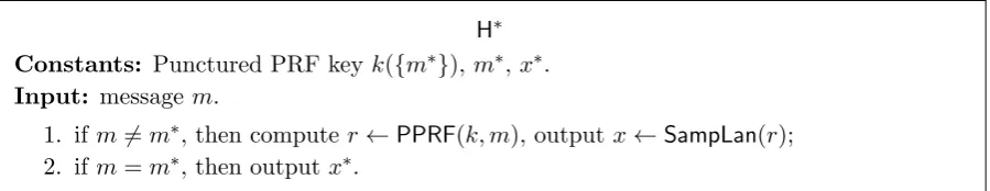
• KeyGen(pp): on inputpp, pick a puncturable PRF keyk∈K as the secret key sk, create an obfuscation of the program of Figure 3 (the size of the program is padded to be the maximum of itself and of Figure 4) as the public key pk.
• PrivEval(sk, x): on input sk and x, output y←PPRF(sk, x).
• PubEval(pk, x, w): on input pk, an element x ∈ L together with its witness w, output
y←pk(x, w).
Public Evaluation
Constants: puncturable PRF keyk.
Input: element x∈ {0,1}2λ, witnessw∈ {0,1}λ.
1. Ifx=PRG(w), outputPPRF(k, x). 2. Else, output ⊥.
Figure 3: Program Public Evaluation
Public Evaluation∗
Constants: puncturable PRF keyk({x∗}).
Input: element x∈ {0,1}2λ, witnessw∈ {0,1}λ.
1. Ifx=PRG(w), outputPPRF(k({x∗}), x). 2. Else, output ⊥.
Figure 4: Program Public Evaluation∗
Theorem 8.1. If the iO is indistinguishably secure,PRGis a secure pseudorandom generator,
and PPRFis selective pseudorandom, then the PEPRFs are adaptive weak pseudorandom.
Proof. The proof follows immediately from [SW14]. Here we only describe the proof in sketch.
To base adaptive weak pseudorandomness of PEPRFs on the security ofPRG, iO, and PPRF, we proceed via a sequence of games where the first game corresponds to the original adaptive weak pseudorandom game for PEPRFs. We prove that A’s advantage must be negligible close between each successive game and that Ahas zero advantage in the final game.
• Setup and challenge: CH runs PEPRF.Setup(1λ) to generate public parameters pp for PEPRFs, runs PEPRF.KeyGen(pp) to generate (pk, sk). CH then picks r∗ ←− {R 0,1}λ,
computes x∗ ← PRG(r∗), sets y0∗ = PrivEval(sk, x∗) and y1∗ ←−R Y, picks a random bit
b∈ {0,1}, and sends (pp, pk, x∗, yb∗) toA as the challenge.
• Evaluation queries: For evaluation queriesx6=x∗,CHanswers with PEPRF.PrivEval(sk, x).
• Guess: Aoutputs its guess b0 and wins ifb0 =b.
Game 1: same as Game 0 with the exception thatx∗ is chosen randomly from {0,1}2λ. Note
thatr∗ is no longer inA’s view and does not need to be generated.
Game 2: same as Game 1 except that the public key is created as an obfuscation of the program Public Evaluation∗ of Figure4.
Game 3: same as Game 2 except that y0∗ is randomly chosen fromY.
Game 0 and Game 1 are computationally indistinguishable assuming the security of the PRG. Game 1 and Game 2 are computationally indistinguishable assuming the security of the un-derlying obfuscation. Game 2 and Game 3 are computationally indistinguishable assuming the selective pseudorandomness of the puncturable PRF. Finally, we observe that any adver-sary’s advantage in Game 3 must be zero, since both y∗0 and y∗1 are randomly chosen from Y. Putting all these together, the desire result immediately follows because the advantage of all PPT adversaries are negligibly close in each successive game.
9
Publicly Sampleable PRFs
In this section, we consider a relaxation of the functionality for PEPRFs, that is, instead of requiring Fsk(x) is publicly evaluable on L, we only require that the distribution (x,Fsk(x))
is efficiently sampleable over L×Y. More precisely, we require there exist a PPT algorithm
PubSampthat on input fresh random coinsr, outputs (x, y)∈L×Y such thaty=Fsk(x). We
refer to this relaxed notion as publicly sampleable PRFs (PSPRFs). Clearly, PEPRFs imply PSPRFs. The (adaptive) weak pseudorandomness for PSPRFs can be defined analogously. It is easy to verify that PSPRFs and KEM imply each other by viewing PSPRF.PubSamp (resp. PSPRF.PrivEval) as KEM.Encaps (resp. KEM.Decaps).10 In light of this observation, we view
PSPRF as a high level interpretation of KEM, which allows significantly simpler and modular proof of security. In what follows, we revisit the notion of trapdoor one-way relations, and explore its relation to PSPRFs.
9.1 Trapdoor Relations
Wee [Wee10] introduced the notion of trapdoor relations (TDRs) as a functionality relaxation of injective TDFs, in which the “easy to compute” property is weakened to “easy to sample”. Wee also showed how to construct such TDRs from EHPSs.
Definition 9.1(Trapdoor Relations). A family of trapdoor relations consists of four polynomial-time algorithms as below.
• Setup(1λ): on input 1λ, output public parameterspp= (R, U, S, P K, SK) (these sets are parameterized by λ), and a collection of binary relations R:U ×S indexed byP K. We say R is one-to-one if for any pk ∈P K, we have: 1) for any s ∈S there exists one and
10
only one u ∈ U such that (u, s) ∈ Rpk; 2) for any u ∈ U there exists at most one s∈ S
such that (u, s)∈Rpk.
• KeyGen(pp): on inputpp, output a public keypk(serve as a key to sample a relation) and a secrey key sk (serve as a trapdoor to find a match).
• TdInv(td, u): on inputtdand u∈U, outputs∈S or a distinguished symbol⊥indicating
u does not have a match underRpk.
• SampRel(pk;r): on inputpk and random coins r, output a tuple (u, s)∈Rpk.
Correctness: For any λ ∈ N, any pp ← Setup(1λ), any (pk, sk) ← KeyGen(pp), and any (u, s)←SampRel(pk), we have (u,TdInv(td, u))∈Rpk.
(Adaptive) One-wayness: Let Abe an inverter against TDRs and define its advantage as:
AdvA(λ) = Pr
(u∗, s)∈Rpk:
pp←Setup(λ);
(pk, sk)←KeyGen(pp); (u∗, s∗)←SampRel(pk);
s← AOinv(·)(pp, pk, u∗)
,
where Oinv(u) = TdInv(sk, u), andA is not allowed to queryOinv(·) for the challenge u∗. We
say TDRs are adaptive one-way (or simply adaptive) if for any PPT inverter its advantage is negligible in λ. The standard one-wayness can be defined similarly as above except that the adversary is not given access to the inversion oracle.
9.2 PSPRFs from TDRs
From one-to-one TDRs, we construct PSPRFs as follows:
• Setup(1λ): run TDR.Setup(1λ) to generate pp = (R, U, S, P K, SK), and let hc :S → Y
be a hardcore function for R; build public parameters pp = (F, P K, SK, X, L, W, Y) for PSPRFs as follows: set P K and SK the same as that of TDRs, set X = U, W = S,
Y = Y, and F will be defined later. R = {Rpk}pk∈P K induces a collection of languages
L = {Lpk}pk∈P K over X = U where each Lpk = {x : ∃w ∈ W s.t. (x, w) ∈ Rpk}. The
corresponding sampling algorithm is the same as that of TDRs. We assume the public parameters pp of TDRs and PEPRFs essentially contains same information.
• KeyGen(pp): on inputpp, output (pk, sk)←TDR.KeyGen(pp).
• PrivEval(sk, x): on input sk and x, output y ← hc(TDR.TdInv(sk, x)). This algorithm defines Fsk :X →Y ∪ ⊥.
• PubSamp(pk;r): on input pk and random coins r, compute (x, w) ← SampRel(pk;r), output (x,hc(w)).
The correctness of the above construction is easy to verify. For the security, we have the following result:
Theorem 9.1. The resulting PSPRFs are (adaptive) weak pseudorandom if the underlying TDRs are (adaptive) one-way.