APPROXIMATE ANALYTICAL SOLUTIONS TO NONLINEAR OSCILLATIONS OF NON-NATURAL SYSTEMS USING HE’S ENERGY BALANCE METHOD
D. D. Ganji, S. Karimpour†,and S. S. Ganji‡
Department of Civil and Mechanical Engineering Babol University of Technology
P. O. Box484, Babol, Iran
Abstract—This paper applies He’s Energy balance method (EBM) to study periodic solutions of strongly nonlinear systems such as nonlinear vibrations and oscillations. The method is applied to two nonlinear differential equations. Some examples are given to illustrate the effectiveness and convenience of the method. The results are compared with exact solutions which lead us showing a good accuracy. The method can be easily extended to other nonlinear systems and can therefore be found widely applicable in engineering and other science.
1. INTRODUCTION
Nonlinear oscillation systems are such phenomena that mostly nonlinearly occur. These systems are important in engineering because many practical engineering components consist of vibrating systems that can be modeled using oscillator systems such as elastic beams supported by two springs or mass-on-moving belt or nonlinear pendulum and vibration of a milling machine [1, 2]. Hence solving of governing equations and due to limitation of existing exact solutions have been one of the most time-consuming and difficult affairs among researchers of vibrations problems. If there is no small parameter in the equation, the traditional perturbation methods cannot be applied directly. Recently, considerable attention has been directed towards the analytical solutions for nonlinear equations without possible small parameters. The traditional perturbation
† Also with Department of Civil and Structural Engineering, Semnan University, Semnan,
Iran
‡ Also with Department of Civil and Transportation Engineering, Azad Islamic University
methods have many shortcomings, and they are not valid for strongly nonlinear equations. To overcome the shortcomings, many new techniques have been appeared in open literature [3–14], such as Non– perturbative methods [3], homotopy perturbation method [4–7, 33– 35], perturbation techniques [8], Lindstedt-Poincar´e method [9, 10], parameter–expansion method [11, 12] and Parameterized perturbation method [13, 14].
Recently, some approximate variational methods, including approximate energy method [15–17, 37, 38], variational iteration method [18–22] and variational approach [23–29, ] and other methods [39], to solution, bifurcation, limit cycle and period solutions of nonlinear equations have been paid much attention.
This paper presents energy balance method (EBM) to study periodic solutions of strongly nonlinear systems. In this method, a variational principle for the nonlinear oscillation is established, then a Hamiltonian is constructed, from which the angular frequency can be readily obtained by collocation method. The results are valid not only for weakly nonlinear systems, but also for strongly nonlinear ones. Some examples reveal that even the lowest order approximations are of high accuracy.
2. ENERGY BALANCE METHOD
In the present paper, we consider a general nonlinear oscillator in the form [17]:
u+f = 0 (1)
in which u andt are generalized dimensionless displacement and time variables, respectively, and f =f(u, u, t).
Its variational principle can be easily obtained:
J(u) =
t
0
−1
2u
2
+F(u)
dt (2)
Its Hamiltonian, therefore, can be written in the form:
H= 1 2u
2
+F(u) =F(A) (3)
Or:
R(t) = 1 2u
2
Oscillatory systems contain two important physical parameters, i.e., the frequencyω and the amplitude of oscillation,A. So let us consider such initial conditions:
u(0) =A, u(0) = 0 (5)
Assume that its initial approximate guess can be expressed as:
u(t) =Acos(ωt) (6)
Substituting Eq. (6) intou term of Eq. (4), yield:
R(t) = 1 2ω
2A2sin2ωt+F(Acosωt)−F(A) = 0 (7)
If by any chance, the exact solution had been chosen as the trial function, then it would be possible to make R zero for all values of t by appropriate choice of ω. Since Eq. (5) is only an approximation to the exact solution,R cannot be made zero everywhere. Collocation atωt=π/4 gives:
ω=
2 (F(A)−F(Acos(π/4)))
A2sin2(π/4) (8)
Its period can be written in the form:
T = 2π
2 (F(A)−F(Acos(π/4))) A2sin2(π/4)
(9)
3. APPLICATIONS OF STRONGLY NONLINEAR VIBRATION SYSTEMS
In this section, we will present three examples to illustrate the applicability, accuracy and effectiveness of the proposed approach.
Example 1. The motion of a particle on a rotating parabola. The governing equation of motion and initial conditions can be expressed as [30]:
1 + 4q2u2d 2u
dt2 + 4q 2u
du dt
2
+ ∆u= 0, u(0) =A, du
where q > 0 and ∆ > 0 are known positive constants [31]. For this problem,f(u) = 4q2u2d2u
dt2 + 4q2u du
dt 2
+ ∆uandF(u) =−2q2u2u2+ 1
2∆u
2. Its variational and Hamiltonian formulations can be readily
obtained as follows:
J(u) =
t 0 −1 2u 2
−2q2u2u2+1 2∆u
2
dt, (11)
H = 1 2u
2
+ 2q2u2u2+1 2∆u
2= 1 2∆A
2, (12)
R(t) = 1 2u
2
+ 2q2u2u2+1 2∆u
2− 1 2∆A
2 = 0, (13)
Substituting Eq. (6) into Eq. (13), we obtain:
R(t) = 1 2A
2ω2sin2(ωt) + 2q2ω2A4cos2(ωt) sin2(ωt)
+1 2∆A
2cos2(ωt)−1 2∆A
2 = 0, (14)
If we collocate atωt=π/4, we obtain the following result:
ω=
∆
(4A2q2cos2(π/4) + 1), (15)
withT = 2ωπ, yield:
T = 2π
∆
(4A2q2cos2(π/4) + 1)
, (16)
Simplifying Eq. (16), gives:
ωEBM =
∆
(2A2q2+ 1), (17)
withT = 2ωπ, yield:
TEBM =
2π
∆ (2A2q2+ 1)
The exact period is [30]:
Tex = 4∆ −1
2 π
2
0
1 + 4q2A2cos2ϕ
1
2 dϕ. (19)
For comparison, the exact periodic solutionsuex(t) achieved by Eqs. (6) and (20), the approximate analytical periodic solutions uEBM(t) computed by Eqs. (6) and (19), are plotted in Figs. 1(a)–(c).
(a) (b)
(c)
Example 2. The motion of a rigid rod rocking back and forth on the circular surface without slipping. The governing equation of motion can be expressed as [30]:
1 12 + 1 16u 2
d2u dt + 1 16u du dt 2 + g
4lucosu= 0,
u(0) =A, du
dt(0) = 0, (20) whereg >0 and l >0 are known positive constants [31].
For the problem, its variational formulation can be obtained as follows:
J(u) =
t 0 −1 2u 2 −3 8u 2u2
+3g(cosu+ sinu) l
dt, (21)
By a similar manipulation as illustrated in previous example by using Eq. (6) and withT = 2ωπ, if we substitutingωt= π/4, we obtain the following result:
R(t) = 1 2A
2ω2sin2(ωt) +3 8A
4ω2cos2(ωt) sin2(ωt)
+
3g(cos (Acos(ωt)) +Acos(ωt) sin (Acos(ωt))
−cos(A)−Asin(A))
l = 0, (22)
ω =
2−6 lg3A2cos2(π/4) + 4(cos(Acos(π/4)) +Acos(π/4) sin(Acos(π/4))−cos(A)−Asin(A)))
(lA(3A2cos2(π/4) + 4) sin(π/4)) , (23)
T = 2π
lA3A2cos2(π/4) + 4sin(π/4)
2−6 lg3A2cos2(π/4) + 4(cos(Acos(π/4)) +Acos(π/4) sin(Acos(π/4))−cos(A)−Asin(A)))
, (24)
Substituting ωt=π/4 into (24), (25), we have:
ωEBM =
4 −3 lg (8 + 3A2) (η)
lA(3A2+ 8) , (25)
TEBM = 2πlA
3A2+ 8
4 −3 lg (8 + 3A2) (η). (26)
whereη is:
η= 2 cos
A√2 2
+A√2 sin
A√2 2
p3 :−δ∂ 2v
3(x, t)
∂x2 +v2(x, t)
∂v0(x, t)
∂x +
∂v2(x, t) ∂t
+v1(x, t)∂v1(x, t)
∂x +v0(x, t)
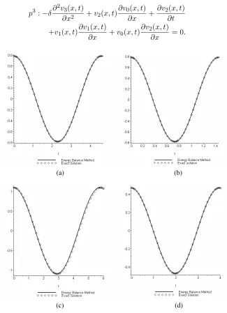
∂v2(x, t) ∂x = 0.
(a) (b)
(c) (d)
The exact period of (20) is:
Tex= 4∆ −1
2 π/2
0
4 + 3A2sin2ϕA2cos2ϕ
8 [AsinA+ cosA−Asinϕsin(Asinϕ)−cos] (Asinϕ)
1 2
dϕ.(28)
The exact period Tex achieved by Eq. (28), the approximate period
TEBM calculated by Eq. (26), are shown in Table 1. Note that for the problem, the maximum amplitude of oscillation should satisfy A < π/2.
Table 1 indicates that Eq. (25) can give an excellent approximate period for oscillation amplitude except those nearA=π/2.
Table 1. Comparison of approximate periods with exact period for Example 2.
A TEBM Tex Error percentage 0.05π 3.66129 3.66109 0.0054
0.10π 3.76397 3.76397 0.0008
0.15π 3.94064 3.94086 0.0056
0.20π 4.20181 4.20292 0.02642
0.25π 4.56432 4.56948 0.1129
0.30π 5.05831 5.07728 0.37348
0.35π 5.73741 5.79770 1.0399
0.40π 6.70586 6.89564 2.7521
0.45π 8.60226 8.94333 3.8136
The exact periodic solutionuex(t) obtained by Eqs. (6) and (28), and the approximate analytical periodic solutions uEBM(t) computed by Eqs. (6) and (25) are plotted in Figs. 2(a)–(d).
4. CONCLUSION
REFERENCES
1. Fidlin, A., Nonlinear Oscillations in Mechanical Engineering, Springer-Verlag, Berlin Heidelberg, 2006.
2. Dimarogonas, A. D. and S. Haddad, Vibration for Engineers, Prentice-Hall, Englewood Cliffs, New Jersey, 1992.
3. He, J. H., “Non-perturbative methods for strongly nonlinear problems,” Dissertation, de-Verlag im Internet GmbH, Berlin, 2006.
4. He, J. H., “Homotopy perturbation technique,” Computer Methods in Applied Mechanics and Engineering, Vol. 178, 257– 262, 1999.
5. He, J. H., “The homotopy perturbation method for nonlinear os-cillators with discontinuities,” Applied Mathematics and Compu-tation, Vol. 151, 287–292, 2004.
6. Hashemi, S. H., H. R. M. Daniali, and D. D. Ganji, “Numerical simulation of the generalized Huxley equation by He’s homotopy perturbation method,” Applied Mathematics and Computation, Vol. 192, 157–161, 2007.
7. Ganji, D. D. and A. Sadighi, “Application of He’s homotopy-perturbation method to nonlinear coupled systems of reaction-diffusion equations,” Int.J.Nonl.Sci.and Num.Simu., Vol. 7, No. 4, 411–418, 2006.
8. Nayfeh, A. H., Introduction to Perturbation Techniques, Wiley, New York, 1981.
9. He, J. H., “Modified Lindstedt–Poincare methods for some strongly nonlinear oscillations, Part I: Expansion of a constant,” International Journal Non-linear Mechanic, Vol. 37, 309–314, 2002.
10. He, J. H., “Modified Lindstedt–Poincare methods for some strongly nonlinear oscillations, Part III: Double series expansion,” International Journal Non-linear Science and Numerical Simula-tion, Vol. 2, 317–320, 2001.
11. Wang, S. Q. and J. H. He, “Nonlinear oscillator with discontinuity by parameter-expansion method,” Chaos & Soliton and Fractals, Vol. 35, 688–691, 2008.
12. He, J. H., “Some asymptotic methods for strongly nonlinear equations,” International Journal Modern Physic B, Vol. 20, 1141–1199, 2006.
perturbation technique,” Communications in Nonlinear Science and Numerical Simulation, Vol. 4, 81–82, 1999.
14. He, J. H., “A review on some new recently developed nonlinear analytical techniques,”International Journal of Nonlinear Science and Numerical Simulation, Vol. 1, 51–70, 2000.
15. He, J. H., “Determination of limit cycles for strongly nonlinear oscillators,”Physic Review Letter, Vol. 90, 174–181, 2006.
16. Ganji, S. S., D. D. Ganji, Z. Z. Ganji, and S. Karimpour, “Periodic solution for strongly nonlinear vibration systems by energy balance method,” Acta Applicandae Mathematicae, doi: 10.1007/s10440-008-9283-6.
17. He, J. H., “Preliminary report on the energy balance for nonlinear oscillations,”Mechanics Research Communications, Vol. 29, 107– 118, 2002.
18. He, J. H., “Variational iteration method — A kind of nonlinear analytical technique: Some examples,” Int.J.Nonlinear Mech., Vol. 34, 699–708, 1999.
19. Rafei, M., D. D. Ganji, H. Daniali, and H. Pashaei, “The variational iteration method for nonlinear oscillators with discontinuities,” Journal of Sound and Vibration, Vol. 305, 614– 620, 2007.
20. He, J. H. and X. H. Wu, “Construction of solitary solution and compaction-like solution by variational iteration method,”Chaos, Solitons & Fractals, Vol. 29, 108–113, 2006.
21. Varedi, S. M., M. J. Hosseini, M. Rahimi, and D. D. Ganji, “He’s variational iteration method for solving a semi-linear inverse parabolic Equation,” Physics Letters A, Vol. 370, 275–280, 2007. 22. Hashemi, S. H. A., K. N. Tolou, A. Barari, and A. J. Choobbasti,
“On the approximate explicit solution of linear and non-linear non-homogeneous dissipative wave equations,” Istanbul Conferences, Torque, accepted, 2008.
23. He, J. H., “Variational approach for nonlinear oscillators,”Chaos, Solitons and Fractals, Vol. 34, 1430–1439, 2007.
24. Naghipour, M., D. D. Ganji, S. H. A. Hashemi, and K. Jafari, “Analysis of non-linear oscillations systems using analytical approach,”Journal of Physics, Vol. 96, 2008.
27. Inokuti, M., et al., “General use of the Lagrange multiplier in non–linear mathematical physics,” Variational Method in the Mechanics of Solids, S. Nemat-Nasser (Ed.), 156–162, Pergamon Press, Oxford, 1978.
28. Liu, H. M., “Generalized variational principles for ion acoustic plasma waves by He’s semi-inverse method,” Chaos, Solitons & Fractals, Vol. 23, No. 2, 573–576, 2005.
29. He, J. H., “Variational principles for some nonlinear partial differential equations with variable coefficient,” Chaos, Solitons and Fractals, Vol. 19, No. 4, 847–851, 2004.
30. Wu, B. S., C. W. Lim, and L. H. He, “A new method for approximate analytical solutions to nonlinear oscillations of nonnatural systems,”Nonlinear Dynamics, Vol. 32, 1–13, 2003. 31. Nayfeh, A. H. and D. T. Mook, Nonlinear Oscillations, Wiley,
New York, 1979.
32. He, J. H., “Variational iteration method — Some recent results and new interpretations,” Journal of Computational and Applied Mathematics, Vol. 207, 3–17, 2007.
33. Dehghan, M. and F. Shakeri, “Solution of an integro-differential equation arising in oscillation magnetic fields using He’s homotopy perturbation method,” Progress In Electromagnetics Research, PIER 78, 361–376, 2008.
34. Bel´endez, A., C. Pascual, S. Gallego, M. Ortu˜no, and C. Neipp, “Application of a modified He’s homotopy perturbation method to obtain higher-order approximations of an force nonlinear oscillator,” Physics Letters A, Vol. 371, 421, 2007.
35. Bel´endez, A., C. Pascual, M. Ortu˜no, C. Neipp, T. Bel´endez,and S. Gallego, “Application of a modified He’s homotopy perturba-tion method to obtain higher-order approximaperturba-tions to a nonlinear oscillator with discontinuities,” Nonlinear Analysis: Real World Applications, 2007, In press.
36. Ganji, S. S., D. D. Ganji, H. Babazadeh, and S. Karimpour, “Variational approach method for nonlinear oscillations of the motion of a rigid rod rocking back and cubic-quintic Duffing oscillators,”Progress In Electromagnetics Research M, Vol. 4, 23– 32, 2008.
37. Pashaei, H., D. D. Ganji, and M. Akbarzade, “Application of energy balance method for strongly nonlinear oscillators,” J. Progress In Electromagnetics Research M, Vol. 2, 47–56, 2008. 38. Akbarzade, M., D. D. Ganji, and H. Pashaei, “Progress analysis of
J.Progress In Electromagnetics Research C, Vol. 3, 57–66, 2008. 39. Vahdati, H. and A. Abdipour, “Nonlinear stability analysis