Distribution of the Cell Under Test in Sliding Window
Detection Processes
Graham V. Weinberg*
Abstract—Radar sliding window detection processes are often used in signal processing as alternatives to Neyman-Pearson based decision rules, due to the fact that they have a simpler receiver implementation and can often be designed to maintain a constant false alarm rate in homogeneous clutter. These detection processes produce a measurement of the clutter level from a series of observations, and compare a normalised version of this to a cell under test. The latter is an amplitude squared measurement of the signal plus clutter in the complex domain. It has been suggested by some authors that that there is sufficient merit in the approximation of the cell under test by a distributional model similar to that assumed for the clutter distribution. This is certainly the case when a Gaussian target is combined with Gaussian clutter, or equivalently a Swerling 1 target and exponentially distributed intensity clutter. The purpose of the current paper is to demonstrate, in a modern maritime surveillance radar context where the clutter is modelled by Pareto statistics, that such an approximation is only valid under certain limiting conditions.
1. INTRODUCTION
The subject under consideration here is whether the cell under test (CUT), in a sliding window detection process operating in high resolution X-band maritime surveillance radar clutter, can be approximated by the same distribution as that used for the clutter, except with different underlying distributional parameters. Sliding window detectors have been of interest to researchers and engineers in radar signal processing for many years [1–3]. These decision rules can often be designed to induce a constant false alarm rate (CFAR) in ideal situations. In recent times the Pareto class of distributions has been validated for the context of interest [4–6]. Based upon this, it has been possible to design, in a systematic way, sliding window detectors for operation in such clutter, with the CFAR property [7].
Sliding window detectors suppose that a series of clutter measurements, denoted asZ1, Z2, . . . , ZN, are available, which are assumed to be non-negative, independent, and identically distributed. A functiong =g(Z1, Z2, . . . , ZN) is then used to produce a single measurement of the clutter level. The CUT is modelled by a non-negative statisticZ0, which is also assumed to be independent of the clutter statistics. The idea is to test whetherZ0 has the same statistical structure as the clutter measurements, or whether it is actually a target embedded within clutter [3]. Suppose thatH0 is the hypothesis that the CUT is just another clutter measurement, and H1 be the hypothesis that the CUT is a target combined with clutter. Then the test can be written
Z0
H1
> <
H0 τ g(Z1, Z2, . . . , ZN), (1)
where τ > 0 is a threshold, and the notation in Eq. (1) means that H0 is only rejected when
Z0 > τ g(Z1, Z2, . . . , ZN). The probability of false alarm (Pfa) of this test is given by
PFA= IP(Z0 > τ g(Z1, Z2, . . . , ZN)|H0). (2)
Received 15 March 2019, Accepted 22 May 2019, Scheduled 27 May 2019
The threshold τ can be determined via Eq. (2), when the distribution of the clutter statistics is given, noting that under H0 the CUT is assumed to also have the same distribution as the clutter measurements. If τ can be determined such that it does not depend on the clutter power then the test in Eq. (1) is such that it can maintain a steady state of false alarms, or equivalently it is said to have the CFAR property.
The problem of interest here is analysis of the CUT in the presence of a target. Some recent studies have suggested that the CUT could be approximated by the same distribution used for the clutter, but with different distributional parameters. This is certainly the case in the context of [1], where the clutter measurements are assumed to be exponentially distributed in intensity, and when a Swerling 1 target model is assumed. The reason this occurs in this context is due to the additivity nature of Gaussian statistics. Extensions of this phenomenon, to non-Gaussian processes, have appeared in the literature. As an example, [8], applied a distributional approximation from [9] for the sum of a series of Weibull distributed variables, to facilitate the derivation of the single measurement of clutter. In addition to this, an approximation is applied for the CUT, relative to the additivity associated with Rayleigh variates. A second, and more recent example, can be found in [10], which suggests that in the case of more modern X-band maritime surveillance radar, the return in the presence of a target can be modelled by a Pareto distribution, which is also used for the clutter measurements. The difference is that the Pareto parameters are modified to account for the presence of a target.
Hence this paper is concerned with the validity of the approximation proposed in [10]. In particular, it is of interest to examine the statistical distribution of the CUT, in the presence of a target, in clutter modelled by Pareto statistics. It will be shown that approximating the CUT by a Pareto type distribution is only valid under very restrictive conditions.
2. THE STRUCTURE OF THE CUT
For the analysis to follow it is necessary to determine mathematically the structure of the CUT in the presence of a target. For analytical tractability it is necessary to assume a particular target model. Here the case of a Gaussian target, embedded in clutter with Pareto intensity statistics, will be examined.
In the complex domain, the CUT consists of a single complex clutter measurement added to a complex target model. Throughout it will be assumed that the target model is bivariate Gaussian. Specifically it is assumed that its in-phase and quadrature components are independent, with zero mean and variance the reciprocal of 2λ, for some λ > 0. This means that the signal power is of the order the reciprocal of λ. This signal is denoted S throughout. For consistency with the currently accepted radar clutter modelling phenomenology, the complex clutter return is assumed to result from a compound Gaussian process with inverse gamma texture, which yields the Pareto Type II clutter model in the intensity realm [7]. Hence the clutter takes the form C=KG, where G is also a bivariate Gaussian process, with independent in-phase and quadrature components, with zero mean and variance the reciprocal of 2μ, for someμ >0. The univariate processK, called the speckle, is assumed to be an independent inverse gamma distributed random variable, with density
fK(t) = β
α
Γ(α)t
−2α−1e−βt−2, (3)
fort >0, where Γ is the gamma function, and α and β are the nonnegative distributional parameters. It can be shown that the intensity random variable I=|C|2 has the Pareto Type II density
fI(t) = αβ
α
(t+β)α+1, (4)
with corresponding distribution function
FI(t) = IP(I ≤t) = 1−
β t+β
α
, (5)
For the target model assumed, it is shown in [11] that the distribution function† of Z is given by
FZ(t) = 1− β
α
Γ(α)
∞
0
uα−1e−βue−
t 1
λ+ 1μudu, (6)
wheret≥0. The problem now is to examine Eq. (6), and determine whether conditions exist, onα, β, λ
and μ, such thatZ has a Pareto Type II distribution.
3. DISTRIBUTION OF THE CUT
This section examines Eq. (6) and derives a Taylor series expansion for it, which facilitates the understanding of the problem under investigation. In the first instance note that the integrand of Eq. (6) can be bounded by uα−1e−βu, for all nonnegative u, t, μ and λ, and that this bound, as a function ofu, is integrable on the real line. Suppose thattandμare fixed. Then Lebesgue’s Dominated Convergence Theorem [12] can be applied to deduce that
lim
λ→∞FZ(t) = 1−
βα
Γ(α)
∞
0
uα−1e−βue−μtudu= 1−
β
μ t+βμ
α
, (7)
where the definition of the gamma function has been used to evaluate the integral. Hence, the distribution function in Eq. (6) limits to that of a Pareto Type II model as the target parameter
λ increases without bound, where the Pareto distribution has shape and scale parameters α and βμ respectively. Thus, when the target vanishes, the result is Pareto distributed clutter in the intensity realm, distributed according to Eq. (7), with an adjusted scale parameter. Using a similar argument, for the case wheret andλare fixed, one can show that
lim
μ→∞FZ(t) = 1−e
−λt, (8)
which is to be expected, since when the Gaussian speckle component vanishes, one is left with a Gaussian signal in the complex domain, which is equivalent to an exponentially distributed target model in the intensity realm.
The limit in Eq. (7) suggests that in the presence of large λ (or equivalently a Swerling target with decreasing variance) that the distribution of the CUT is roughly Pareto Type II. In order to gain further insight into this, it is worth examining Eq. (6) in more detail. In particular, an expression will be derived for the latter to show its relationship to Eq. (7) in explicit detail.
Towards this objective, note that it is the third term in the integrand in Eq. (6) which results in the integral being difficult to evaluate. Hence define a function
g(u) =
1
λ+
1
μu
−1
−1
= λμu
μu+λ. (9)
Then the third term in the integrand of Eq. (6) is
T =e−g(u)t. (10)
With application of the Taylor series expansion for the exponential function, it follows that
T =
∞
k=0 (−1)k
k! g
k(u)tk. (11)
By applying the ratio test [13], one can show that this power series is absolutely convergent everywhere. Therefore, applying Eq. (11) to Eq. (6), one arrives at
FZ(t) = 1− β
α
Γ(α)
∞
k=0 (−1)k
k! t
k(λμ)k ∞
0
uα+k−1e−βu
[μu+λ]k du. (12)
Switching the order of summation and integration is justified on the basis that the power series is absolutely convergent everywhere [13].
A second Taylor series expansion is now applied to Eq. (12); towards this define a function
h(u) = [μu+λ]−k. (13)
The nth derivative ofh(u) with respect tou is given by
dh(u)
du = (−1)
nk(k+ 1)(k+ 2)· · ·(k+n−1)[μu+λ]−k−nμn. (14)
Observing thath(0) =λ−k the Taylor series for h(u) about 0 is therefore given by
h(u) =λ−k+
∞
n=1
(−1)nk(k+ 1)(k+ 2)· · ·(k+n−1)
n! λ
−k−nμnun. (15)
Through an application of the ratio test for power series, it can be demonstrated that this power series is absolutely convergent provided
1
λ<
1
μ. (16)
Under the assumption that condition (16) holds, one can apply this Taylor series to Eq. (12), and switch the order of summation and integration within the circle of convergence of the power series, to obtain
FZ(t) = 1− β
α
Γ(α)
∞
k=0 (−1)k
k! t
kμk×
∞
0
uα+k−1e−βudu+
∞
n=1
(−1)nk(k+1)(k+2)· · ·(k+n−1)
n!
μn λn
∞
0
uα+k+n−1e−βudu
.(17)
The two integrals that appear in Eq. (17) can be recognised as gamma integrals, which can be evaluated in terms of gamma functions. Hence it is not difficult to show that Eq. (17) is reduced to the form
FZ(t) = 1− 1 Γ(α)
∞
k=0 (−1)k
k! μt β k ×
Γ(α+k) +
∞
n=1 (−1)n
k+n−1
n
Γ(α+k+n)
μ λβ
n
= 1− 1 Γ(α) ∞ k=0 (−1)k k! μt β k
Γ(α+k)
− 1
Γ(α)
∞
k=0 (−1)k
k! μt β k ∞ n=1
(−1)nk+n−1 n
Γ(α+k+n)
μ λβ
n
, (18)
where the permutation in Eq. (17) has been converted to a combination coefficient. Firstly consider the component
G(t) := 1− 1 Γ(α)
∞
k=0 (−1)k
k!
μt β
k
Γ(α+k). (19)
One can show, by constructing a Taylor series expansion around the point t= 0, that
μt β + 1
−α
= 1 +
∞
k=1
(−1)kα(α+ 1)· · ·(α+k−1)
k! μt β k . (20)
With an application of the ratio test, one can show that this power series is absolutely convergent under the condition
β
Assuming this is the case, it then follows that G(t) is exactly the limiting distribution function in Eq. (7).
Next attention is focused on the component
H(t) :=− 1 Γ(α)
∞
k=0 (−1)k
k!
μt β
k ∞
n=1 (−1)n
k+n−1
n
Γ(α+k+n)
μ λβ
n
. (22)
By changing the index nto m=n−1 one can express Eq. (22) in the form
H(t) =
μ λβ
∞
k=0 (−1)k
k!
μt β
k ∞
m=0
(−1)mΓ(α+k+m+ 1) Γ(α)
k+m m+ 1
μ λβ
m
. (23)
Notice that for fixedt, the function H is of the order 1λ. Hence the decomposition
FZ(t) =G(t) +H(t) (24)
consists of a Pareto Type II distribution function, independent of λ, and an offset component, which decreases to zero as λ increases. This decomposition is valid provided conditions (16) and (21) hold. Condition (16) is stipulating the target power is smaller than the speckle power, while condition (21) is requiring the product of the Pareto clutter scale parameter and the speckle power to exceed unity.
The conclusion from these results is that the distribution function in Eq. (6) is only Pareto distributed in the limit as λ increases. To obtain further insight into why it may be believed that the distribution ofZ is approximately Pareto distributed, it is worth considering the asymptotic study of the Pareto distribution in [14]. In many cases the underlying clutter environment may limit to an exponential distribution. As an example, in the case of vertically polarised clutter returns, as the Pareto shape parameter increases, the exponential approximation of the Pareto model becomes valid. If this is the case in practice, then the additivity property of the Gaussian model may be observed, and it may result in the conclusion that a Gaussian target, in Pareto distributed clutter, is approximately Pareto distributed. However, this is really a result of the limiting behaviour reported in [14].
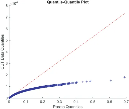
To illustrate these results, two quantile plots are examined. In this situation, the underlying Pareto clutter distribution is assumed to have parameters α = 4.7241 and β = 0.0446. A Gaussian target for the CUT is assumed, withμ= 1, and the CUT is simulated by generating a compound Gaussian model with inverse gamma texture, added to the complex version of a Gaussian target model. Figure 1 shows
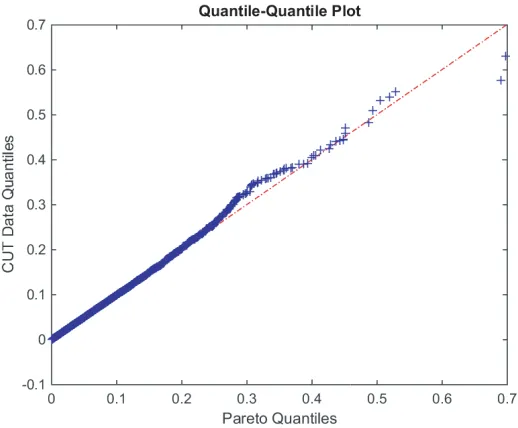
Figure 2. Quantile comparison for the situation of smaller SCR (−50 dB), or equivalently, large λ. Here the CUT is approximately Pareto distributed.
the quantile plot of the simulated CUT, when the target has signal to clutter ratio (SCR) of 50 dB. The latter quantity, in absolute units, varies directly as the reciprocal of the square root of λdefined above. The horizontal axis if for the Pareto distributional intensity measurements, while the vertical axis plots the CUT quantiles. Here one observes that the distribution of the CUT is not Pareto, since the quantiles deviate from a straight line. Figure 2 changes the SCR to −50 dB, and here one observes that the distribution of the CUT is closer to Pareto, due to the suppression of the Gaussian target.
4. CONCLUSION
It was shown that the distribution of signal plus clutter could be decomposed into a limiting Pareto Type II component, and a component which decreased to zero as the target’s variance also decreased to zero. Hence the distribution function examined could only be considered to be approximately Pareto distributed when the target’s power is very small relative to the speckle’s power. Observed results in the literature, suggesting this approximation is valid beyond this condition, may be a by-product of the limiting behaviour of the Pareto model.
REFERENCES
1. Finn, H. M. and R. S. Johnson, “Adaptive detection model with threshold control as a function of spatially sampled clutter-level estimates,”RCA Review, Vol. 29, 414–464, 1968.
2. Gandhi, P. P. and S. A. Kassam, “Analysis of CFAR processors in nonhomogeneous background,” IEEE Transactions on Aerospace and Electronic Systems, Vol. 24, 427–445, 1988.
3. Minkler, G. and J. Minkler, CFAR: The Principles of Automatic Radar Detection in Clutter, Magellan, 1990.
4. Balleri, A., A. Nehorai, and J. Wang, “Maximum likelihood estimation for compound-Gaussian clutter with inverse-Gamma texture,” IEEE Transactions on Aerospace and Electronic Systems, Vol. 43, 775–779, 2007.
5. Farshchian, M. and F. L. Posner, “The Pareto distribution for low grazing angle and high resolution X-band sea clutter,”IEEE Radar Conference Proceedings, 789–793, 2010.
7. Weinberg, G. V., Radar Detection Theory of Sliding Window Processes, CRC Press, New York, 2017.
8. Siddiq, K. and M. Irshad, “Analysis of the cell averaging CFAR in Weibull background using a distributional approximation,” 2nd International Conference on Computer, Control and Communication, 2009.
9. Dong, Y., “Distribution of X-band high resolution and high grazing angle sea clutter,” Defence Science and Technology Organisation Research Report, 2006.
10. Persson, B., “Radar target modeling using in-flight radar cross section measurements,”Journal of Aircraft, Vol. 54, 284–291, 2017.
11. Weinberg, G. V., “Constant false alarm rate detectors for pareto clutter models,” IET Radar, Sonar and Navigation, Vol. 7, 153–163, 2013.
12. Bartle, R. G., The Elements of Integration and Lebesgue Measure, Wiley, New York, 1995. 13. Kaplan, W., Advanced Calculus, Addison-Wesley, Massachusetts, 1984.