Parametric Study of Vertical Ground Loop Heat Exchangers for Ground Source Heat Pump Systems

(1)

Scholarship@Western

Electronic Thesis and Dissertation Repository

2-2-2016 12:00 AM

Parametric Study of Vertical Ground Loop Heat Exchangers for

Ground Source Heat Pump Systems

Abdelrahman S. Ramadan

The University of Western Ontario

Supervisor

Dr. Karman Siddiqui

The University of Western Ontario

Graduate Program in Mechanical and Materials Engineering

A thesis submitted in partial fulfillment of the requirements for the degree in Master of Engineering Science

Follow this and additional works at: https://ir.lib.uwo.ca/etd

Recommended Citation Recommended Citation

Ramadan, Abdelrahman S., "Parametric Study of Vertical Ground Loop Heat Exchangers for Ground Source Heat Pump Systems" (2016). Electronic Thesis and Dissertation Repository. 3521.

https://ir.lib.uwo.ca/etd/3521

This Dissertation/Thesis is brought to you for free and open access by Scholarship@Western. It has been accepted for inclusion in Electronic Thesis and Dissertation Repository by an authorized administrator of

(2)

Abstract

We report on a numerical study conducted to investigate the effect of various parameters

on the heat exchange inside a vertical ground loop heat exchanger (VGLHE) for a

ground-source heat pump (GSHP) system. The simulations were conducted for three

piping configurations of the ground loop which were U-Tube, Concentric pipes and

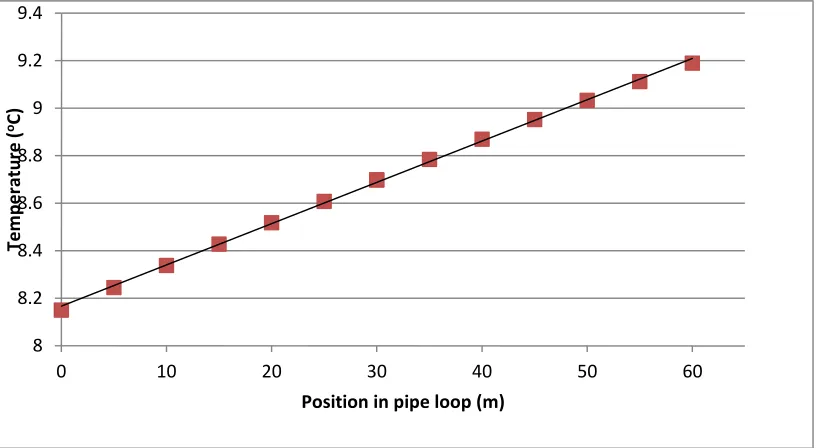
Spiral. The results show a linear temperature rise along the pipe length for the U-Tube

configuration. The concentric pipes configuration shows two distinct linear trends for the

temperature rise; a slow temperature rise during the downward flow through the inner

pipe and a higher temperature rise during the upflow through the annulus. The spiral

configuration shows a steeper slope for the temperature rise in the spiral section and

almost a flat slope for the temperature rise in the straight vertical section of the pipe. The

research also examines a simulation case of integrating a VGLHE inside a micro-pile

foundation system.

Keywords

Ground source heat pumps, vertical ground loop heat exchanger, numerical modelling,

computational fluid dynamics, ANSYS FLUENT, micro-pile, geothermal, parametric

(3)

Statement of Originality

This is to certify that, to the best of my knowledge, the content of this thesis is my own

work. This thesis has not been submitted for any degree or other purposes.

I certify that the intellectual content of this thesis is the product of my own work and that

all the assistance received in preparing this thesis and sources have been acknowledged.

(4)

Acknowledgments

I would like to express my gratitude and appreciation for both my supervisor Dr. Kamran

Siddiqui and co-supervisor Dr. Hesham El-Naggar for their guidance, support and, above

all, patience to help me complete my research and thesis. I’m grateful to their efforts in

enhancing my knowledge and research skills as well as giving me the chance to

participate in various technical conferences which added to my graduate experience.

I’m extremely thankful to my whole family who supported and motivated me in every

step of the way of this long journey, especially my father.

Finally, and most importantly, I’m indebted to my wife Dima for her encouragement,

support, quiet patience and unending love. I dedicate all my work to you and to our new

(5)

List of Tables

Table 2-1: Geometrical dimensions of 3D model ... 39

Table 2-2: Properties of different mesh sizes used for mesh dependency test ... 41

Table 2-3: Boundary conditions used in mesh dependency test ... 41

Table 2-4: Thermophysical properties of material used in simulation ... 41

Table 2-5: Outlet temperature for different mesh sizes ... 42

Table 2-6: Physical dimensions of experimental borehole ... 45

Table 2-7: Thermophysical properties of materials used in the experiment ... 45

Table 2-8: Operating conditions and properties for thermal response test ... 46

Table 3-1: Thermophysical properties of material used in simulation ... 51

Table 3-2: Boundary conditions used [Adopted from Esen et al. 2009] ... 51

Table 3-3: Area-weighted average surface heat flux values for different pipe sections ... 55

Table 3-4: Calculated thermal resistances of individual VGLHE components ... 59

Table 3-7: Summary of simulation results for three different piping configurations ... 74

Table 3-8: Summary of simulation results for different pipe materials in concentric pipe configuration. ... 76

(9)

Table 3-10: Summary of simulation results for concentric piping configurations with

varying volume flow rate of heat transfer fluid ... 81

Table 3-11: Parameters and dimensions of micro-pile used in simulation ... 86

(10)

List of Figures

Figure 1.1: World energy consumption in quadrillion Btu, 1990-2040 [EIA 2013] ... 2

Figure 1.2: World energy consumption by fuel type, 1990-2040 (quadrillion Btu) [EIA

2013] ... 2

Figure 1.3: Total US energy consumption by sector in 2013 [US DOE 2013] ... 3

Figure 1.4: Percentage distribution of solar energy [Omer 2008] ... 4

Figure 1.5: Depth dependence of annual range of ground temperatures in Ottawa, Canada

[Williams and Gold 1976] ... 5

Figure 1.6: Work and heat flow balance for a heat pump [NRC 2005] ... 6

Figure 1.7: Refrigeration cycle of a typical heat pump unit [NRC 2005] ... 6

Figure 1.8: Typical GHE loop configurations for GSHP systems. a) Vertical closed GHE

configuration, b) Horizontal closed GHE configuration and c) Open loop groundwater

configuration. [NRC 2005] ... 7

Figure 1.9: Top view and side view of a single pipe U-Tube piping configuration in a

VGLHE. ... 9

Figure 1.10: Cross section of a U-tube borehole and corresponding thermal circuit ... 11

Figure 1.11: Typical side views of a) End Bearing Pile and b) Friction Pile [Beardmore

2012] ... 15

Figure 1.12: Typical hollow bar micro-pile (Drbe et al. 2013) ... 17

Figure 1.13: Photo of a typical reinforcement cage for a foundation pile integrated with

high density polyethylene piping [BINE IS, 2010] ... 19

Figure 1.14: Photo of the integrated reinforcement cage inserted inside the pile borehole

(11)

Figure 2.1: A schematic diagram showing horizontal and vertical cross sections of a

vertical U-tube GHE (Development of a numerical model for the simulation of vertical

U-tube ground heat exchangers) ... 26

Figure 2.2: Section view of simulated components and type of heat transfer ... 33

Figure 2.3: Algorithm illustrating steps of a Pressure-Based solution ... 36

Figure 2.4: Top view and side view of U-Tube piping geometry domain used in simulation. ... 37

Figure 2.5: Top isometric view of the vertical ground loop 3D geometry ... 37

Figure 2.6: Bottom isometric view of the vertical ground loop 3D geometry ... 38

Figure 2.7: Top isometric view of generated mesh ... 40

Figure 2.8: Plot of wall y+ along depth of pipe (top 0.5m) ... 42

Figure 2.9: Entrance length for fluid flow for mesh #4 ... 43

Figure 2.10: Schematic of an in-situ test setup (adapted from Esen et al [2009]) ... 44

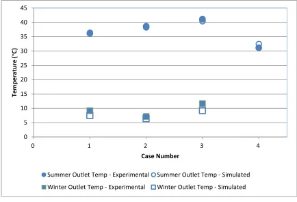
Figure 2.11: Comparison between experimentally measured and numerically simulated fluid outlet temperatures ... 47

Figure 3.1: Top view and side view of U-Tube piping geometry domain used in simulation. ... 50

Figure 3.2: Temperature of fluid along the pipe ... 52

Figure 3.3: Temperature distribution in the borehole horizontal plane at depths of (a) 0 m, (b) 10 m, (c) 20 m, (d) 30 m . The colour bar represents the temperature in degree Celsius. ... 54

(12)

Figure 3.5: Temperature profile of fluid at different depths of down-flow pipe ... 57

Figure 3.6: Sketch indicating the location of temperature data points ... 58

Figure 3.7: Normalized temperature profile of fluid at different depths of down-flow pipe

... 58

Figure 3.8: (a) Temperature and (b) velocity contours of the bottom bend of pipe ... 60

Figure 3.9: Top view and side view of concentric piping geometry domain used in

simulation. ... 62

Figure 3.10: Area-averaged temperature of fluid along the pipe ... 63

Figure 3.11: Temperature distribution in the borehole horizontal plane at depths of (a) 0

m, (b) 10 m, (c) 20 m, (d) 29 m. The colour bar represents the temperature in degree

Celsius. ... 65

Figure 3.12: : Temperature distribution in the fluid horizontal plane at depths of (a) 0 m,

(b) 10 m, (c) 20 m, (d) 29 m. The colour bar represents the temperature in degree Celsius.

... 66

Figure 3.13: (a) Temperature and (b) velocity contours in the bottom section of the

concentric pipe ... 67

Figure 3.14: Isometric view of 3D model of spiral piping configuration simulated ... 69

Figure 3.15: Average temperature of fluid along the length of loop ... 70

Figure 3.16: Temperature distribution in the borehole horizontal plane at depths of (a) 0

m, (b) 2 m, (c) 4 m, (d) 6 m, (e) 8 m, (f) 10 m. The colour bar represents the temperature

in degree Celsius. ... 71

Figure 3.17: Temperature distribution in the fluid horizontal plane at depths of (a) 0 m,

(b) 2 m, (c) 4 m, (d) 6 m, (e) 8 m, (f) 10 m. The colour bar represents the temperature in

(13)

Figure 3.18: Temperature of fluid at different positions of the pipe for three different

piping configurations ... 74

Figure 3.19: Average fluid temperature along full length of concentric piping for four

cases with different piping materials. ... 77

Figure 3.20: Temperature of fluid along full length for three concentric piping

configurations with changing grout thermal conductivity values ... 80

Figure 3.21: Temperature of fluid along full length for three concentric piping

configurations with changing fluid volume flow rates values ... 82

Figure 3.22: Typical hollow bar micro-pile (Drbe et al. 2013) ... 84

Figure 3.23: Top view and side view of energy micro-pile geometry domain used in

simulation. ... 85

Figure 3.24: Ground temperature profile for the Goderich area in south western Ontario

(Markle, 2011) ... 87

(14)

List of Symbols

c

o_C

Specific Heat Capacity, J/kg K

Celsius Degree

C1𝜖 Constant (experimentally determined)

C2 Constant (experimentally determined)

COPh/c Design Heating/Cooling Coefficient of Performance

DH Hydraulic Diameter, m

E Total Energy Transported, J

Fh/c Part load factor (full load hours to total number of hours in design month)

𝑔⃗ Gravitational Acceleration Constant, m/s2

Gb Generation of turbulence kinetic energy due to buoyancy

Gk Generation of turbulence kinetic energy due to the mean velocity gradient

k Turbulence Kinetic Energy

Keff Effective Thermal Conductivity, W/(m°K)

Le Entrance Length, m

𝑚̇

p

Mass Flow Rate, kg/s

Pressure, Pa

Prt Prandtl number

QC Heat extracted from the cold reservoir, kW

QH Heat added to the hot reservoir, kW

Re Reynolds Number

Rp Pipe Thermal Resistance, °K/W

Rs Soil Thermal Resistance, °K/W

S Modulus of the mean rate-of-strain tensor

(15)

Tewt,min/max Minimum/Maximum design entering water temperature, °C

Tg,min/max Minimum/Maximum undisturbed ground temperature, °C

TI Turbulent Intensity

Ti Temperature data point in the mid vertical plane, oC

Tinlet Fluid Inlet Temperature, oC

Toutlet Fluid Outlet Temperature, oC

𝑣⃗ Velocity, m/s

W Work input, kW

x Cartesian x coordinate

y Cartesian y coordinate

YM Contribution of the fluctuating dilatation in compressible turbulence to the

overall dissipation rate

z Cartesian z coordinate

Greek Symbols

µt Turbulent Viscosity

ϵ Dissipation Rate

μ Dynamic Viscosity, kg/m·s

ρ Density, kg/m3

σk Turbulent Prandtl numbers for k (Turbulence Kinetic Energy)

σϵ Turbulent Prandtl numbers for ϵ (Dissipation Rate) 𝜏̿̅ Stress Tensor

(16)

List of Abbreviations

CFD Computational Fluid Dynamics

COP Coefficient of Performance

EIA Energy Information Administration

GHE Ground Heat Exchanger

GSHP Ground Source Heat Pump

HDPE High Density Poly Ethylene

HT Fluid Heat Transfer Fluid

SIMPLE

TRT

Semi-Implicit Method for Pressure-Linked Equations

Thermal response Test

UDF User Defined Function

USDOE US Department of Energy

(17)

Chapter 1 : INTRODUCTION

1

Introduction

1.1 Background

The 2013 International Energy Outlook published by the U.S. Energy Information

Administration (EIA) projected a continuous increase in the world energy consumption

levels over the next few decades [EIA 2013]. As shown in Figure 1.1, it is estimated that

the world energy consumption will grow by approximately 56% between 2010 and 2040.

Different energy sources will be required to meet this increasing demand and as can be

seen by Figure 1.2, fossil fuels (oil, coal and gas) are predicted to account for

approximately 75% of the world energy consumption by 2040 [EIA 2013]. This fossil

fuel dependency outlook is most certainly reinforced by the recent drop in crude oil

prices globally. The heavy reliance on fossil fuels combined with the fact that burning

fossil fuels produces greenhouse gases such as nitric oxide and carbon dioxide, has

generated growing concerns related to the environmental impacts of these fuels. It is

estimated that the world energy-related carbon dioxide emissions will increase by

approximately 36% by 2040 (due mainly to non-OECD countries) [EIA 2013]. This

massive global energy consumption has always demanded engineers, scientists and

designers to explore other renewable resources and more efficient systems.

The largest energy consuming sector in the U.S. is the building sector (consisting of

residential and commercial buildings). As shown in Figure 1.3, it is estimated that

approximately 40%of total U.S. energy consumption in 2013 (97.4 Quadrillion Btu) was

utilized by buildings, which was higher than each of the other two remaining sectors,

transportation and industrial [US DOE 2013]. Approximately 50% of the total energy

consumed by buildings is used for space heating and air conditioning [EIA 2013]. This

presents a major potential opportunity for utilizing renewable energy sources for space

heating and cooling, which reduces the use and current dependency on fossil fuels and

(18)

Figure 1.1: World energy consumption in quadrillion Btu, 1990-2040 [EIA 2013]

(19)

Figure 1.3: Total US energy consumption by sector in 2013 [US DOE 2013]

One of these potential renewable energy sources is the earth’s ground energy, which is

utilized via a Ground Source Heat Pump (GSHP) system with considerable economic

advantages and cost savings. The GSHP system operates on the basis of using ground as

a heat source for heating purposes in winter and as a heat sink for cooling purposes in

summer. It is argued that geothermal heating systems can be more efficient than electric

resistance heating, gas or oil-fired heating systems and air-source heat pumps [Omer

2008].

Although GSHP systems could be viewed as attractive and feasible from the energy cost

point of view, the installation costs associated with the drilling of the boreholes

containing the ground heat exchangers could be prohibitive and could act as a barrier for

increasing the use and installation of beneficial GSHPs. Nonetheless, relatively novel

methods have been explored in order to reduce this premium installation cost and one of

these methods is the “Energy Pile” system where it utilizes the building structural

foundation piles as ground heat exchangers.

In the next sections a background for GSHP and energy pile systems will be presented as

(20)

1.2 Ground Source Heat Pump (GSHP) Systems

It has been well established that the main source of energy on earth is solar radiation

[Phillips 1995], which also serves as the source for many global energy sources available

to us including solar energy, wind energy, petrochemical and more importantly

geothermal and earth-energy systems. Considering that almost half of the sun’s solar

energy gets absorbed by earth as shown in Figure 1.4, it seems logical to utilize this

abundant storage of renewable energy that is readily available on site all year long.

Figure 1.4: Percentage distribution of solar energy [Omer 2008]

With that solar energy being stored underground as thermal energy, the soil also acts as

an insulator between the ambient air above ground and the earth below. This insulation

produces a constant ground temperature below a certain depth all year round that is

independent of the above ground air temperatures that fluctuate due to seasonal variations

as shown in Figure 1.5. The temperature of the ground at shallower depths may not be

constant; however, their fluctuations are greatly reduced when compared to the ambient

(21)

Therefore, the temperature of the ground below a certain depth is warmer than the

ambient air in winter and is cooler than the ambient air in summer. This is the basis of

operation for ground source heat pump systems (GSHP) where heat can be absorbed from

the relatively warm ground in winter and rejected into the relatively cool ground in the

summer through the use of ground source heat pumps.

1.2.1 Components of a GSHP System

Ground source heat pump systems consist of three main components:

1- Heat pump machine:

The ideal heat pump “pumps” heat from a cold source to a hot reservoir through the

application of work as shown in Figure 1.6 below (opposed to the natural flow of heat

from hot to cold). This cycle is known as the vapour compression refrigeration cycle and

is typical for any heat pump whether ground-source, water-source, or air-source as shown

in Figure 1.7.

(22)

Figure 1.6: Work and heat flow balance for a heat pump [NRC 2005]

Figure 1.7: Refrigeration cycle of a typical heat pump unit [NRC 2005]

The function of the heat pump in a GSHP system is to transfer the heat between the earth

connection and the heating/cooling distribution system. The most common kind of

GSHPs is the “water-to-air” where the heat carried by the fluid from and to the earth

connection is ultimately transferred to and from the air distribution system within the

building. If the distribution system is hydronic (heating/cooling water loop) then the

(23)

All of the heat pump components shown are usually contained in one enclosure and the

enclosure itself is placed indoors in a furnace room or a mechanical room. Typical

capacities for GSHPs range from 3.5kW to 35kW [NRC 2005].

2- Heating/Cooling distribution system:

This is the distribution system which delivers heating or cooling to the building of

interest. The distribution system is usually the conventional air duct or hydronic (hot

water) piping distribution system.

3- Earth connection:

The earth connection is the ground loop piping system that acts as the heat exchanger

between the ground and the GSHP system. There are two ground heat exchanger (GHE)

systems; closed loop and open loop systems. Within each system there are different

configurations of the underground piping loop layouts: vertical, horizontal, coiled,

surface water and open system wells. Some examples are shown in Figure 1.8 below.

Figure 1.8: Typical GHE loop configurations for GSHP systems. a) Vertical closed GHE configuration, b) Horizontal closed GHE configuration and c) Open loop groundwater configuration. [NRC 2005]

In the closed loop systems, the GSHP system circulates a heat transfer fluid, usually

water or an antifreeze glycol mixture from the heat pump machine to the ground loop and

(24)

water from the designated well or aquifer to the heat pump and then returns it back to the

environment through injection wells.

In the present research, the type of GHE of interest is the vertical closed loop type,

hereinafter referred to as “Vertical Ground Loop Heat Exchanger” or “VGLHE”, and

therefore more related information will be presented here.

1.2.2 Vertical Ground Loop Heat Exchanger (VGLHE)

A typical Vertical Ground Loop Heat Exchanger (VGLHE) consists of three key

components, as shown in the single pipe U-tube configuration in Figure 1.9:

1- Heat Transfer Fluid

2- Piping

3- Grout material

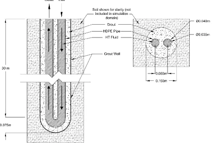
The depth and diameter of the boreholes containing the VGLHE vary from case to case

depending on many specific factors, such as the peak heating load, peak cooling load,

number of VGLHEs in a system, thermal properties of the soil and others. However, the

diameter and depth of the borehole generally range from 100 mm to 150 mm and from 15

m to 120 m, respectively [GSHPA 2007].

The piping material commonly used in GSHP installations is High Density Polyethylene

(HDPE) and the pipe nominal sizes typically range from 20 mm 40 mm. The function of

the piping is to convey the heat transfer fluid, typically water or an anti-freeze mixture, to

circulate into and out of the VGLHE from and back to the heat pump equipment. There

are different configurations of the piping other than the common single pipe U-tube

configuration, such as the concentric piping, spiral piping and the double pipe U-tube

(25)

Figure 1.9: Top view and side view of a single pipe U-Tube piping configuration in a VGLHE.

The third component surrounding the piping is the grout. The grout prevents the ground

water from the risk of contamination and provides a thermal connection to the

surrounding soil. It is for the latter reason that the grout material is preferable to a have a

high thermal conductivity value. Typical geothermal grout material is a bentonite grout

mixture.

1.2.3 Relevant Parameters and Factors:

The efficiency of any heat pump including GSHPs is measured by a parameter called the

coefficient of performance (COP). The COP is the ratio of change in heat at the reservoir

of interest to work input in the process. Generally ground source heat pumps have heating

COPs ranging from 2.4 to 5.0 and cooling COPs ranging from 3.1 to 8.8 [Rafferty et al

(26)

Heating and cooling COPs are calculated using the following equations:

𝑄_𝐻= 𝑊 + 𝑄_𝐶 Eq. 1-1

𝐶𝑂𝑃_{𝐻𝑒𝑎𝑡𝑖𝑛𝑔} = 𝑈𝑠𝑒𝑓𝑢𝑙 𝐻𝑒𝑎𝑡𝑖𝑛𝑔 𝑒𝑛𝑒𝑟𝑔𝑦

𝐶𝑜𝑚𝑝𝑟𝑒𝑠𝑠𝑜𝑟 𝑎𝑛𝑑 𝐹𝑎𝑛 𝑎𝑛𝑑 𝑃𝑢𝑚𝑝 𝐸𝑛𝑒𝑟𝑔𝑦 =

𝑊 + 𝑄𝐶

𝑊 Eq. 1-2

𝐶𝑂𝑃𝐶𝑜𝑜𝑙𝑖𝑛𝑔 =

𝑈𝑠𝑒𝑓𝑢𝑙 𝐶𝑜𝑜𝑙𝑖𝑛𝑔 𝑒𝑛𝑒𝑟𝑔𝑦

𝐶𝑜𝑚𝑝𝑟𝑒𝑠𝑠𝑜𝑟 𝑎𝑛𝑑 𝐹𝑎𝑛 𝑎𝑛𝑑 𝑃𝑢𝑚𝑝 𝐸𝑛𝑒𝑟𝑔𝑦 =

𝑄_𝐶

𝑊 Eq. 1-3

Where:

𝑄_𝐶 is the amount of heat extracted from the cold reservoir

𝑄𝐻 is the amount of heat added to the hot reservoir

𝑊 is the work input

Another important objective when designing for a GSHP system is the proper sizing of

the GHE length. This is a critical consideration since the capital costs of GSHP system

are higher than conventional systems. Below are the relevant equations from a simplified

method from the International Ground Source Heat Pump Association (IGSHPA)

[IGSHPA 1988]:

Sizing based on the heating load: 𝐿ℎ = 𝑞𝑑,ℎ𝑒𝑎𝑡[

(𝐶𝑂𝑃_ℎ− 1)

𝐶𝑂𝑃ℎ (𝑅𝑝+ 𝑅𝑠𝐹ℎ)

𝑇𝑔,𝑚𝑖𝑛− 𝑇𝑒𝑤𝑡,𝑚𝑖𝑛

] Eq. 1-4

Sizing based on the cooling load: 𝐿𝑐 = 𝑞𝑑,𝑐𝑜𝑜𝑙[

(𝐶𝑂𝑃_𝑐 − 1)

𝐶𝑂𝑃𝑐 (𝑅𝑝+ 𝑅𝑠𝐹𝑐)

𝑇𝑒𝑤𝑡,𝑚𝑎𝑥− 𝑇𝑔,𝑚𝑎𝑥

] Eq. 1-5

Where:

COPh/c is the design heating/cooling coefficient, respectively

Tg,min/max is the minimum/maximum undisturbed ground temperature

Tewt,min/max is the minimum/maximum design entering water temperature

(27)

Rs is the soil thermal resistance

Fh/c is the part load factor (full load hours to total number of hours in design month)

The design entering water temperatures are estimated using the following equations

[Kavanaugh et al 1997]:

𝑇_{𝑒𝑤𝑡,𝑚𝑖𝑛} = 𝑇_{𝑔,𝑚𝑖𝑛}− 15𝑜𝐶 Eq. 1-6

𝑇𝑒𝑤𝑡,𝑚𝑎𝑥 = 𝑚𝑖𝑛 (𝑇𝑔,𝑚𝑎𝑥+ 15𝑜𝐶, 43𝑜𝐶) Eq. 1-7

1.2.4 Heat transfer modes in boreholes

In a borehole, the heat exchange takes place between the soil and the heat transfer fluid

which serve as the temperature nodes. The heat flows between these two nodes from the

higher temperature node to the lower temperature node. During its passage from one node

to the other, the heat flow experiences resistances, which influence the magnitude of the

heat transfer rate. These resistances which are also termed as “thermal resistances”

depend on the material properties as well as the flow behaviour (when present).

The thermal resistance of a borehole at a 2D section can be represented through a thermal

circuit as shown in Figure 1.10.

(28)

Tf1 and Tf2 are the temperatures of the heat transfer fluid in pipe 1 and pipe 2,

respectively.

Rf1 and Rf2 are the convective thermal resistances between the flowing fluid and the pipe

within pipe1 and pipe 2, respectively.

Tp1,i and Tp2,i are the temperatures of the inner surface of pipe1 and pipe 2, respectively.

Rp1 and Rp2 are the wall conductive thermal resistances of pipe 1 and pipe 2, respectively.

Tp1,o and Tp2,o are the temperatures of the outer surface of pipe1 and pipe 2, respectively.

Rg is the conductive thermal resistance within the grout body.

Tg is the average wall temperature of borehole’s grout wall.

Rs is the conductive thermal resistance of the surrounding soil.

Ts is the average temperature of the surrounding soil.

The figure shows a 2D heat transfer process and two heat fluxes, q1 and q2. q1 is the heat

transferred between the soil and the fluid in pipe 1, and q2 is the heat transferred between

the soil and the fluid in pipe 2.

For the purposes of this research the simulation domain has been selected to include only

the fluid, piping, and grout. The research excluded the soil effect or behaviour as

described later in section 2.2. Based on that, the soil temperature, Ts, and soil thermal

resistance, Rs, will be excluded from this analysis.

As shown in Figure 1.10, the total thermal resistance between the fluid nodes and the

grout wall consists of conductive and convective resistances. These thermal resistances

are defined by the following equations.

The resistance of the fluid is calculated using the following equation [Drake et al 1972]:

R

_f1

=

1

2𝜋𝑟1𝑖ℎ1

,

R

f2

=

1

2𝜋𝑟2𝑖ℎ2 Eq. 1-8

Where,

h1 and h2 are the convective heat transfer coefficients of the fluid inside pipe 1 and pie 2, respectively

(29)

The resistance of the pipe is calculated using the following equation [Drake et al 1972]:

𝑅

_𝑝1

=

𝑙𝑛(𝑟1𝑜

𝑟1𝑖)

2𝜋𝑘

,

𝑅

𝑝2

=

𝑙𝑛(𝑟2𝑜

𝑟2𝑖)

2𝜋𝑘

,

Eq. 1-9

Where,

k is the thermal conductivity of the pipe

r1o and r2o are the outside radii of pipe 1 and pipe 2, respectively

The thermal resistance of the grout involves 2D heat transfer consideration since the

source/sink is embedded within the grout. This calculation requires the computation of

the conduction shape factor, which is based on the configuration and dimensions of the

heat source/sink (Incropera 2007). Rg could also be calculated from the average

temperature profile at the wall of the borehole and the surface of the U-tube pipes using

the following equations [Hellström, 1991]:

𝑅

_𝑔

=

𝑇

𝑔

− 𝑇

𝑝1,𝑜

𝑞

₁

=

𝑇

_𝑔

− 𝑇

_𝑝2,𝑜

𝑞

₂ Eq. 1-10

The overall heat transfer rates q1 and q2 can then be described using the following equations:

𝑞₁= 𝑇𝑔− 𝑇𝑓1

𝑅_𝑔 + 𝑅_𝑝1 + 𝑅_𝑓1 Eq. 1-11

𝑞₂ = 𝑇𝑔− 𝑇𝑓2

𝑅𝑔+ 𝑅𝑝2+ 𝑅𝑓2

Eq. 1-12

1.3 Energy Piles – Fundamentals

As mentioned earlier, Energy Piles systems are basically thermal foundation piles which

serve both as a structural foundation for the building and as a ground energy heat

exchanger for GSHP systems. This section provides the background description on

(30)

1.3.1 Pile foundations - Background

Pile foundations are deep building foundations that transfer the structural load from the

building to the soil layers below, which can provide the required load bearing capacity.

They generally consist of long, slim and columnar elements installed into the ground. A

pile foundation is different from a shallow foundation and typically has a depth that is

more than three times its width [Atkinson 2007]. Piles are commonly constructed from

reinforced concrete, steel or timber and are usually used for large building structures or in

situations where the shallow soil is just not suitable for a shallow foundation structure.

Based on the functions of the pile foundations, they could be classified into two types as

shown in Figure 1.5 below:

1- Friction pile foundation: The load bearing capacity of each pile is provided by

the shear stresses developed by the contact between the sides of the piles and

the soil.

2- End bearing pile foundation: The majority of the load bearing capacity is

developed at the bottom “toe” of the pile.

The ultimate load-carrying capacity of a pile, Qu, is given by the equation [Atkinson 2007]:

𝑄_𝑢 = 𝑄_𝑝+ 𝑄_𝑠 Eq. 1-13

Where:

Qp is the load-carrying capacity of the pile’s bottom “toe”

Qs is the frictional resistance derived from soil-pile interface

The end-bearing capacity, Qp, is given by the following equation [Atkinson 2007]:

(31)

Where:

Ap is the area of pile tip

c’ is the cohesion of the soil supporting the pile tip

qp is the unit point resistance

q’ is the effective vertical stress at the level of the pile tip 𝑁_𝑐∗,𝑁_𝑞∗ are the bearing capacity factors

Figure 1.11: Typical side views of a) End Bearing Pile and b) Friction Pile [Beardmore 2012]

The frictional, or skin, resistance of the pile is given by the following equation [Atkinson

2007]:

𝑄_𝑠 = ∑ 𝑝∆𝐿𝑓 Eq. 1-15

Where:

p is the perimeter of the pile section

Load Pile Cap

Pile

Friction

(32)

∆L is the incremental pile length over which p and f are taken to be constant

f is the unit friction resistance at any depth z

The installation and construction of foundation piles can be broken down to two methods:

1- Driven piles: The steel or concrete pile structure is delivered to site and then

vertically driven into the soil through the action of a driving hammer machine

(falling weight impact on the top of the pile).

2- Bored piles: In this installation method, the soil is extracted (bored) out of the

ground first and then the concrete mixture is poured into the hole. Other variants

include extraction of the soil out of the ground and pouring and pumping of the

concrete mixture simultaneously [O'Sullivan, 2001].

The selection of the pile installation method depends on many site specific factors, such

as the soil conditions, type of building structure, cost and available area of construction.

1.3.1.1 Micro-Pile System

One specific pile foundation type of system, the Micro-Pile, will be given more attention

in this section as it will be used in a computational fluid dynamics (CFD) case simulation

in later chapters.

Micro-Piles in general are deep foundation piles that typically have small diameters (less

than 300 mm) [Wynne 1988]. They were initially conceived to underpin historic

buildings and monuments but they have evolved ever since to become a common

foundation option for new construction projects as well. They have a main advantage

over other deep foundation systems when installation sites have limited access or low

headroom due to the smaller installation and drilling equipment required.

As shown in Figure 1.12, a typical hollow bar micro-pile consists mainly of a sacrificial

drill bit at the bottom, a threaded steel hollow bar (the pile body itself), couplers to extend

the overall length of the micro-pile and the grouting around the steel pile to provide the

(33)

As the ground hole or pile shaft is being drilled by the sacrificial drill bit, the hollow core

bar is advanced into the required depth of the drilled hole. High strength grouting

material is then pumped inside the hollow bar and after passing through one or more

nozzles in the sacrificial drill bit, it diffuses and fills up the gap between the pile and the

ground [Liew et al, 2003]. Although the function of the grouting around the pile is to bind

the outside surface of the threaded steel hollow bar to the adjacent soil, the typical end

product usually has the grouting inside of the hollow bar steel pile.

(34)

1.3.2 Energy Piles

Energy piles are basically foundation piles that incorporate a closed loop VGLHE system

within it to act as a heat sink in the heating season and a heat source in the cooling

season. The energy pile is ultimately connected to the GSHP system serving the building.

The main advantage of an energy pile system over a conventional GSHP system is that

the foundation structure that houses the ground heat exchanging system is already

required for structural purposes and the VGLHE does not need to be drilled or

constructed separately [Suryatriyastuti et al, 2012].

This structural and thermal multi-purpose feature of the energy pile system can eliminate

the prohibitive high installation cost associated with the drilling of dedicated boreholes

for the GHSP system and thus reducing the premium installation cost. Another advantage

of the energy pile system is the reduction of the land use which originally would have

been required for a conventional GSHP system.

1.3.2.1 Construction of Energy Piles

Historically, the structural components of a building to be utilized for ground heat

transfer applications were foundation slabs. Overtime, other types of structural

components such as bored piles, precast driven piles and diaphragm walls were

effectively developed to be used for heating and cooling applications [Thompson III,

2013]. The use of bored piles with large diameters has been increasing over the past

decade and is believed to have overtaken the use of prefabricated driven piles in these

heat transfer applications [Brandl, 2006].

Typical foundation piles are transformed to energy piles by retrofitting the inside of each

pile with one or more loops of high density polyethylene (HDPE) piping along its depth.

Regardless of the geothermal requirements, the length and diameter of the pile should be

sized and designed based on the applied structural load and the skin friction required to

resist.

The drilling and excavation of the soil in a bored energy pile is usually performed by

(35)

depth of the energy pile is achieved. The liquid concrete or grout is then pressurized and

pumped into the freshly drilled borehole through an outlet port on the tip of auger while it

is slowly being withdrawn and risen. This is done in order to ensure the structural

capacity of the pile is not compromised by vacancies in the pile.

The piping loops are typically attached and strapped onto the welded pile reinforcement

cage, shown in Figure 1.13, which is then inserted and lowered into the borehole

following the drilling and the removal of the soil, as shown in Figure 1.14. The

reinforcement cage can be inserted before or after the liquid concrete has been poured

into the borehole. The piping loops are usually internally pressurized before being

inserted into the liquid concrete filled borehole to protect the piping from damage and to

ensure the piping inner cross section is not crimped to allow for unrestricted flow for the

heat transfer fluid once put in operation.

(36)

Figure 1.14: Photo of the integrated reinforcement cage inserted inside the pile borehole [Skanska, 2011]

1.4 Literature Review

There are relatively few studies reported in the literature that investigated the heat

transfer in VGLHEs and due to the cost and logistics, mostly comprised of numerical

approaches. Furthermore, these studies were focused on a particular geometry or

condition and hence, there is a lack of comprehensive parametric studies investigating the

effects of main parameters (such as geometry, operational and thermo-physical

properties) on the performance of VGLHEs. Lenhard et al. [2013] performed a

Computational Fluid Dynamics (CFD) simulation on a double U-tube VGLHE utilizing

the k-ε turbulence model. The only parameter of comparison used in this study was the

depth of the VGLHE where the effects on the circulating fluid were analysed at different

depths ranging from 50 m to 147 m (mesh dependency test was not demonstrated in the

study). The simulation results showed that the total heat transfer rate inside the VGLHE

increased linearly with depth and at a higher rate than that of the soil temperature. He et

al. [2012] presented a numerical 3D modelling study of a single U-tube VGLHE in both

transient and steady-state stages. The study tested and evaluated the effect of the fluid

flow rates on the fluid outlet temperature and the total heat flux. They observed that the

(37)

depth, were linear at relatively high fluid flow rates and noticeably non-linear at

mid-range and low fluid flow rates. The study also looked at the inter-tube heat flux, also

called “short-circuit” heat flux, between the upward and downward fluids flowing in the

adjacent U-tube pipes and estimated it to be inversely proportional to the flow velocity.

The simulation, however, assumed a constant ground temperature along the depth of the

borehole.

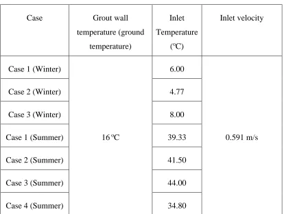
Esen et al. [2009] conducted an experimental study analysing the effect of the borehole

depth on the overall COP of the GSHP system. The experimental work included an

in-situ Thermal Response Test (TRT) for a ground source heat pump system in Elazig,

Turkey. It used an above ground pump with a heater circulating heat transfer fluid

through the borehole piping while continuously measuring the fluid temperatures at the

inlet and outlet of the borehole. The experiment looked at both summer and winter modes

of operations. The study produced well documented data and readings applicable for

CFD simulations. The authors have also conducted other studies validating the results of

the presented experiments using Artificial Neural Network (ANN) and Adaptive

Neuro-fuzzy Inference System (ANFIS) models [Esen et al 2010].

Gustafsson et al. [2010] conducted numerical investigation of two different VGLHE

geometries, U-tube and concentric, using the ANSYS FLUENT software. The results of

the numerical simulations were compared with published laboratory experiments. Unlike

conventional U-tube borehole configuration, they modelled the U-tube immersed in the

groundwater (instead of the conventional grout) followed by the surrounding soil. The

study was primarily focused on the influence of the induced velocity flow in the

surrounding groundwater due to the temperature gradient and the resulting density

differences. They found that the induced natural convection in the groundwater

significantly decreased the thermal resistance of the borehole. The VGLHE models in

this study were only 3 metres deep and no direct comparison of the performances

between the two different geometries was performed.

Bidarmaghz et al. [2013] studied the effects on the heat extraction rate of a VGLHE

(38)

piping configuration and geometry. The piping configurations that were simulated were

the single U-tube, double U-tube and double cross U-tube. The results showed that the

magnitude of the heat extraction rate increased at a high rate as the flow rate of the fluid

was increased within the laminar regime (low Reynolds numbers). However, above a

certain flow rate and when the flow became turbulent, the magnitude of the heat

extraction rate increased at a slower rate compared to that in the laminar regime. As for

the effect of the piping configuration, the results showed that the double U-tube piping

configuration achieved between 40% to 90% higher extraction rate when compared to the

single tube piping configuration of the same depth. The double and the double cross

U-tube piping configurations showed very similar heat extraction rates when the fluid flow

was in the laminar and transitional flow regimes, however, in the turbulent flow regime,

the double U-tube piping configuration resulted in a 23% increase in the heat extraction

rate.

Recently, Gashti et al. [2014] performed a 3D numerical simulation for heating/cooling

operations of a ground heat exchanger incorporated within a steel pile foundation (energy

pile). The results of the simulation were compared with those of a 20 m deep

experimental energy pile with two different types of piping configurations (single U-tube

and double U-tube) under different fluid flow rates. The study showed good agreement

between the simulated and experimental performance of the energy pile which validated

the simulation model. Analysis of the results indicated that an increase in the number of

piping loops inside of the energy pile is more efficient than increasing the diameter of the

pipes themselves (double U-tube systems performed better than single U-tube systems).

This improved performance ranged from 10% to 60% depending of the fluid flow rate.

The study also revealed that systems with small differences between tube inlet and

ground temperatures had little difference in their power output and implied that higher

temperature differences between the inlet fluid and ground temperature are required to

achieve tangible differences in the power output.

Zarrella et al. [2014] used the equivalent thermal resistance and capacitance circuit

approach to model heat transfer in an energy pile. The model was validated with field

(39)

between helical and a triple U-tube configuration inside the energy pile was conducted.

The results showed that helical-pipe energy piles performed better thermally than the

conventional tube configuration. In addition, the performance of a standard double

U-tube borehole heat exchanger was compared with the modelled two energy pile

configurations. As expected, the thermal performance of the double U-tube heat

exchanger was lower than both energy pile configurations (30% lower than the

helical-pipe energy pile and 13% lower than the triple U-tube one).

Cvetkovski [2014] conducted a detailed numerical study and simulation on the fluid flow

and heat transfer behaviour at the bottom 180o bend of a U-tube VGLHE. The study

investigated the effect of Reynolds and Dean Numbers on the fluid flow and heat

transfer. It utilized the ANSYS FLUENT software package and the realizable k-ϵ

turbulence model to solve the associated flow and heat transfer equations. The results

were validated with the values provided from experimental testing. The study concluded

that in additional to redirecting the fluid flow back up, the 180o bend generated Dean’s

vortices which enhanced the heat transfer significantly overall and particularly in that

location. Decreasing the fluid flow velocity was found to decrease the resident time for

heat transfer at the bend and hence a reduction in the outlet temperature.

1.5 Motivation and Objectives

The motivation for this research is to better understand and ultimately optimize the

performance of Ground Source Heat Pump systems especially when these systems are

integrated in an energy pile structure. There are many geometrical, thermo-physical, and

operational parameters that could highly affect the heat exchange process between the

VGLHE and the soil and hence, the COP of the whole system. For instance, there are

several piping loop configurations that could be installed inside a VGLHE or an energy

pile such as the U-tube, concentric and the spiral piping configuration with each

configuration producing different fluid outlet temperatures and total heat transfer rates.

As the above literature review shows, there is a lack of detailed parametric study to

investigate the effects of these parameters on the heat transfer process. The understanding

of these effects is vital in order to improve the design and selection process for GSHPs

(40)

Objectives

The main objectives of this proposed study are:

1- To develop a numerical 3D CFD model simulating the heat transfer process inside

a Vertical Ground Loop Heat Exchanger (VGLHE) for a Ground Source Heat

Pump (GSHP) system.

2- To conduct a parametric study using the developed numerical 3D model to further

understand the heat transfer process and draw comparisons for different piping

configurations, materials of construction and fluid flow rates.

1.6 Thesis Format and Layout

This thesis consists of four chapters. Chapter 1 provides an introduction and background

information on the Ground Source Heat Pump (GSHP) system and Energy Piles,

literature review, and motivation and objectives for this research. Chapter 2 describes the

3D numerical model that was developed including the modelling process, geometry,

mesh generation and validation. Chapter 3 presents the detailed parametric study along

with the comparison and discussion of its results. Finally, Chapter 4 presents the

(41)

Chapter 2 : NUMERICAL MODEL

2

Numerical Model

This chapter describes the 3D numerical model that was developed in order to simulate

the proposed heat exchange processes in a Vertical Ground Loop Heat Exchanger

(VGLHE) system. The specifics and geometry for the model are based on typical

VGHLEs. This chapter begins with a description of the geometry of interest followed by

the description of governing mathematical equations and models utilized for simulations.

The chapter will then present the mesh dependency test results, followed by the model

validation.

2.1 Modelling Process

As mentioned in the previous chapter, the main focus of this research is the vertical

ground loop heat exchanger (VGLHE) component of the ground source heat pump

system. This is where the heat transfer occurs between the ground and the GSHP system

and has the direct impact on the heat pump system performance. The ground heat transfer

process occurs within four main components that make up a typical VGLHE (shown in

Figure 2.1):

1- Surrounding soil

2- Grout

3- Piping

(42)

Figure 2.1: A schematic diagram showing horizontal and vertical cross sections of a vertical U-tube GHE (Development of a numerical model for the simulation of vertical U-tube ground heat exchangers)

2.2 Exclusion of Soil Modelling

A complete soil model analysis would need to include the following effects:

1- Impact of thermal cycling on the bond strength between the grout and the

surrounding soil. As the operational mode of the system switches between cooling

and heating every year and due to thermal expansion and contraction, it’s

expected that the bond strength between the grout and the soil will be impacted.

This is more relevant for energy pile applications where the pile’s structural strength is dependent on its “skin” friction.

2- Impact of water content or ground water in the soil on the thermal conductivity of

the grout material. As the overall size of the borehole may change (due to thermal

expansion) there’s the possibility of the grout absorbing some of the water content

in the surrounding soil over time. This would affect the thermal conductivity of

(43)

For the purposes of this research the simulation domain has been selected to include only

the fluid, piping, and grout. The research excluded the soil effect or behaviour on the

performance of the VGLHE. This assumption was used to focus on the effects of varying

internal VGLHE parameters, such as geometric, thermophysical and operational

parameters on the overall performance while maintaining the exterior ground conditions

unchanged. In addition, the work in this thesis focuses on the individual performance of

the VGLHE and not the group effect; hence, the soil model could be neglected since it’s

more relevant when evaluating the interactions between multiple VGLHEs. This

exclusion also reduces the large computation time and resources required.

A wall temperature boundary condition was set for the model on the outer grout wall to

simulate the temperature of the surrounding soil.

2.3 Numerical Model Development and Formulation

The physical modelling and meshing were constructed using the default ANSYS

modeller and mesher while the simulations were solved using FLUENT 14.0.

FLUENT is a numerical solver with modelling capabilities for incompressible and

compressible, transient and steady-state, laminar and turbulent fluid flow problems

[FLUENT 2010]. It’s very versatile in the way it allows the user to easily change

boundary conditions and parameters while producing accurate simulation results.

In this section the governing mathematical equations, models and numerical assumptions

implemented in the developed model are described.

2.3.1 Continuity and Momentum Equations

All CFD simulations are founded on the solution of governing equations which describe

the behaviour of the flow. The CFD solver numerically solves the mass (Continuity) and

momentum conservation (Navier-Stokes) equations along with other additional transport

equations depending on the complexity of the flow (e.g. energy conservation, species

mixing or reactions, turbulent flow). The turbulence and heat transfer governing

(44)

equations and other related terms presented in this Chapter that provide the model

description are obtained from the FLUENT user manual [FLUENT 2010].

The conservation of mass equation, or continuity equation, has the following general

form:

𝜕𝜌

𝜕𝑡 + ∇ ∙ (𝜌𝑣⃗) = 𝑆𝑚 Eq. 2-1

For incompressible (ρ ~ constant) and steady state flow as in the present case, the first term on the left in Eq. (2.1) can be neglected. Likewise, the source term on the right side

of the equation, Sm, can be neglected since no mass is being added from a dispersed phase to another continuous phase. Thus, in the present case, this equation reduces to:

∇ ∙ (𝑣⃗) = [𝜕𝑣𝑥

𝜕𝑥 +

𝜕𝑣_𝑦

𝜕𝑦 +

𝜕𝑣𝑧

𝜕𝑧] = 0 Eq. 2-2

Where 𝑣⃗𝑥 , 𝑣⃗𝑦 and 𝑣⃗𝑧 are the velocity components of the fluid in x, y and z, directions, respectively.

The conservation of momentum equation, in an inertial (non-accelerating) reference

frame, is described as follows:

𝜕

𝜕𝑡(𝜌𝑣⃗) + ∇ ∙ (𝜌𝑣⃗𝑣⃗) = −∇p + ∇ ∙ (𝜏̅̿) ∙ 𝜌𝑔⃗ Eq. 2-3

Where p is the static pressure, 𝜌𝑔⃗ is the gravitational body force and 𝜏̅̿ is the stress tensor

defined as:

𝜏̅̿ = 𝜇 [(∇𝑣⃗ + ∇𝑣⃗𝑇_{) −}2

3∇ ∙ 𝑣⃗𝐼] Eq. 2-4

(45)

2.3.2 Turbulence Model

The fluid flow regime inside the piping of ground source heat pump systems is turbulent

in nature due to the high Reynolds number, Re, which is defined as

𝑅𝑒 =𝜌𝑣(𝐷𝐻)

𝜇 Eq. 2-5

Where DH is the hydraulic diameter which is equal to the physical pipe diameter for a circular pipe, v is the mean velocity of the fluid, ρ is the density of the fluid and µ is the dynamic viscosity of the fluid.

The Reynolds number for a given fluid flow is used to classify the flow regime. The flow

is considered to be laminar if the Reynolds Number is lower than 2,000 and turbulent if it

is higher than 5,000. Between these two limits, the flow regime would be considered in a

transitional phase [White 2002]. In the base case for which we are initially applying the

geometrical and operational parameters from an experimental VGLHE testing apparatus

[Esen et al 2009], the Reynolds Number was calculated to be 11,270. This calculation

considered a density of 1017 kg/m3, an inlet velocity of 0.591 m/s, a hydraulic diameter

(pipe inner diameter) of 30 mm and a dynamic viscosity of 0.0016 𝑘𝑔 𝑚∙𝑠.

FLUENT offers three main categories for turbulent flow simulation methods. These are:

 DNS – Direct Numerical Simulation

 SRS – Scale Resolving Simulations

 RANS – Reynolds Averaged Navier-Stokes Simulations

The first two categories, DNS and SRS, are usually best fit for unsteady flow conditions

and complex flow patterns. The RANS turbulence models are the only meddling

approach for steady stage simulation of turbulent flows and they provide the required

(46)

Within the RANS category, FLUENT further provides an array of models for the steady

state calculations. These models are generally divided between “one-equation” and “two-

equations” models. Of these steady state models, the realizable k-ε model is selected. The

k-ε model is considered to be one of the simplest “complete models” of turbulence where the solution of two separate transport equations allows the turbulent velocity and length

scales to be independently determined. Due to its robustness and reasonable accuracy, it

has become commonly used in industrial flow and heat transfer simulations since it was

proposed by Launder et al. (1972).

The realizable k-𝜖 turbulence model has also been utilized for very similar VGLHE simulations by other researchers [Cvetkovski 2014, Congedo et al. 2014] with accurate

results. It is a recent development from the standard k-ε model which is a semi-empirical model based on the solution of two separate transport equations for the turbulence kinetic

energy (k) and the energy dissipation rate (𝜖). The realizable model differs from the standard one in the way it formulates the turbulent viscosity (µt) and it also has a new transport equation for the energy dissipation rate (𝜖).

The main two transport equations used to obtain the turbulence kinetic energy (k) and its rate of dissipation (ε) are:

𝜕 𝜕𝑡(𝜌𝑘) + 𝜕 𝜕𝑥_𝑗(𝜌𝑘𝑢𝑗) = 𝜕 𝜕𝑥_𝑗[(𝜇 + 𝜇_𝑡 𝜎_𝑘) 𝜕𝑘

𝜕𝑥_𝑗] + 𝐺𝑘+ 𝐺𝑏− 𝜌𝜖 − 𝑌𝑀 Eq. 2-6

𝜕 𝜕𝑡(𝜌𝜖) + 𝜕 𝜕𝑥𝑗 (𝜌𝜖𝑢_𝑗) = 𝜕 𝜕𝑥𝑗 [(𝜇 +𝜇𝑡 𝜎𝑘 ) 𝜕𝜖 𝜕𝑥𝑗

] + 𝜌𝐶₁𝑆_𝜖− 𝜌𝐶₂ 𝜖

2

𝑘 + √𝑣𝜖+ 𝐶1𝜖

𝜖

𝑘𝐶3𝜖𝐺𝑏 Eq. 2-7

Where,

𝐶₁ = 𝑚𝑎𝑥 [0.43, 𝜂

𝜂 + 5] , 𝜂 = 𝑆

𝑘

𝜖, 𝑆 = √2𝑆𝑖𝑗𝑆𝑖𝑗 Eq. 2-8

In the above transport equations:

 Gk is the generation of turbulence kinetic energy due to the mean velocity gradient

(47)

 YM is the contribution of the fluctuating dilatation in compressible turbulence to

the overall dissipation rate.

 C1εand C2 are constants that are experimentally determined and have the

following values: C1ε=1.44, C2=1.9

 S is the modulus of the mean rate-of-strain tensor

 σk and σε are the turbulent Prandtl numbers for k and ϵ, respectively. They are

experimentally determined and have the following values: σk=1.0, σε=1.2

 µt is the turbulent viscosity, defined as 𝜇𝑡 = 𝜌𝐶𝜇𝑘2

𝜖 where 𝐶𝜇 = 1

𝐴0+𝐴𝑠𝑘𝑈∗_𝜖

where 𝑈∗ ₌_{̅ √𝑆}

𝑖𝑗𝑆𝑖𝑗+ Ω̃𝑖𝑗Ω̃𝑖𝑗

and Ω̃_𝑖𝑗 = Ω_𝑖𝑗 − 2𝜖_𝑖𝑗𝑘𝜔_𝑘

Ω𝑖𝑗 = Ω̅𝑖𝑗 − 𝜖𝑖𝑗𝑘𝜔𝑘

Ω̅_𝑖𝑗 is the mean rate-of-rotation tensor in a rotating reference frame with angular

velocity ωk.

A0 and As are constants: 𝐴0 = 4.04 and 𝐴𝑠 = √6𝑐𝑜𝑠𝜙 where

𝜙 =1

3𝑐𝑜𝑠

−1_{(√6𝑊), 𝑊 =}𝑆𝑖𝑗𝑆𝑗𝑘𝑆𝑘𝑖

𝑆̃3 , 𝑆̃ = √𝑆𝑖𝑗𝑆𝑖𝑗, 𝑆𝑖𝑗 =

1 2( 𝜕𝑢𝑗 𝜕𝑥𝑖+ 𝜕𝑢𝑖 𝜕𝑥𝑗)

2.3.3 Energy and Convective Heat Transfer Modelling

Due to the presence of heat transfer in our simulations, the turbulent model selected in

FLUENT also models the turbulent heat transport using the notion of Reynolds’

similarity to the turbulent momentum transfer. The energy equation used is given as

[FLUENT 2010]: 𝜕 𝜕𝑡(𝜌𝐸) + 𝜕 𝜕𝑥𝑖 [𝑢𝑖(𝜌𝐸 + 𝑝)] = 𝜕 𝜕𝑥𝑗

(𝑘_eff 𝜕𝑇

𝜕𝑥𝑗

+ 𝑢_𝑖(𝜏_𝑖𝑗)

eff) + 𝑆ℎ Eq. 2-9

(48)

 E is the total energy transported,

 Sh is the defined volumetric heat source,

 keff is the effective thermal conductivity and

 (τij)eff is the deviatoric stress tensor defined as:

(𝜏_𝑖𝑗)

eff= 𝜇eff (

𝜕𝑢_𝑗

𝜕𝑥_𝑖 +

𝜕𝑢𝑖

𝜕𝑥_𝑗) −

2

3𝜇eff

𝜕𝑢𝑘

𝜕𝑥_𝑘𝛿𝑖𝑗 Eq. 2-10

 keff, the effective thermal conductivity in the above equation, is defined as

𝑘_eff = 𝑘 +𝑐𝑝𝜇𝑡

Pr_t Eq. 2-11

Where, k represents the thermal conductivity of the material and Prt is Prandtl number.

2.3.4 Energy Modelling in Solid Regions

As the present case consists of two solid components, pipe and grout, the proposed model

will need to solve the energy equations in these solid regions. The energy transport

equation used by FLUENT is the following:

𝜕

𝜕𝑡(𝜌ℎ) + ∇ ∙ (𝑣⃑𝜌ℎ) = ∇ ∙ (𝑘∇T) + 𝑆ℎ Eq. 2-12

Where ρ = Density

h = Sensible Enthalpy, ∫_{𝑇𝑟𝑒𝑓}𝑇 𝑐_𝑝𝑑𝑇

k = conductivity

T = Temperature

Sh = Volumetric Heat Source

Since the flow being simulated is steady and incompressible (ρ ~ constant), the first term on the left in Eq. (2.9) can be neglected. The second term on the left, which represents the

(49)

be neglected since the pipe and grout solid components are motionless. This equation

simulates the conductive heat transfer in the solid regions.

2.3.5 Conjugate Heat Transfer

As the present modelling domain contains a fluid/solid interface involving heat transfer,

the solver will need to simulate it as a conjugate heat transfer problem. The FLUENT

solver computes the conduction of heat through solids, coupled with convective heat

transfer in the fluid. Generally, the Navier Stokes and the convective energy equations in

the fluid region (Heat Transfer Fluid) are solved first followed by the conductive heat

transfer equations in the solid regions (pipe and grout). Figure 2.2 outlines the locations

of each solid and fluid region as well as the fluid/solid interface wall.

The pipe/fluid wall is considered a “two-sided-wall” since it forms the interface between the two regions. It is there where a “shadow” zone is created so that each side of the wall

is a distinct wall zone. Then a “Coupled Thermal Condition” is applied and the solver

calculates the heat transfer directly from the solution in the adjacent cells. Pipe Grout

Fluid Flow

Grout Wall Grout/Pipe Wall

Pipe/Fluid Coupled Wall (Solid/Fluid) Conductive

Convective

(50)

At the boundary condition definition stage, the walls are selected to be “coupled” and any

resistance parameter set for one side of the wall will automatically be assigned to its

shadow wall zone.

2.3.6 Boundary Conditions

A critical component of any CFD simulation is the setting up of appropriate thermal and

physical parameters on the physical boundaries of the model. FLUENT provides a range

of boundary condition types and this section describes those that were selected for this

model.

2.3.6.1 Inlet and outlet boundary conditions

A velocity inlet boundary condition was selected at the pipe inlet. The magnitude and

direction of velocity, fluid temperature, hydraulic diameter and turbulent intensity are the

variables required to fully define the inlet velocity boundary condition. All of these

variables are provided by the model’s physical properties except for the turbulent

intensity, TI, which is related to the Reynolds number, Re, in the following manner [FLUENT 2010]:

𝑇𝐼 = 0.16 𝑅𝑒−1/8

The boundary type at the pipe outlet in the model was selected to be a pressure outlet

boundary condition with turbulent intensity factor and hydraulic diameter variables

identical to those considered for the inlet boundary conditions.

2.3.6.2 Walls

The fluid adjacent walls were set as stationary with no-slip conditions. The external grout

walls were set with a constant temperature boundary condition representing the

temperature of the soil.

Also, it must be noted that all of the simulations in this research were considered to be

conjugate heat transfer problems due to the interface between the fluid region (heat

(51)

selecting the “Coupled” option for the two-sided walls in the thermal conditions setting

within the software.

2.3.7 Solution Methods and Initialization

Based on previous research and simulations conducted by other researches on similar

types of flow problems, the FLUENT solver selected for this model was the

pressure-based solver, which is intended for low-speed incompressible flows [FLUENT 2010].

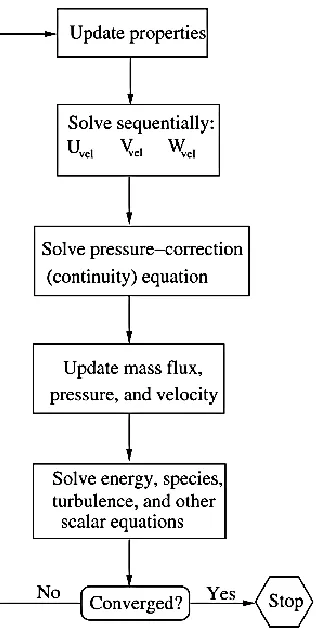
The segregated pressure-based scheme SIMPLE, Semi-Implicit Method for

Pressure-Linked Equations, was used which utilizes the relationship between velocity and pressure

corrections to impose the mass conservation (continuity) and find the pressure field. The

steps used in the algorithm are illustrated in Figure 2.3. The convergence criterion was set

at 10-3 for the continuity equation, 10-4 for the axial velocity, 10-4 for k and ε, and 10-5 for the energy (temperature) equation. The criterion for each parameter has been selected and

evaluated based on the steady behaviour of the resultant residual plot.

The gradients were computed according to the “Least Squares Cell Based” method. The

spatial discretization scheme used to evaluate pressure, momentum, turbulent kinetic

energy, turbulent dissipation rate, and energy quantities was the “Second Order Upwind”

scheme. This scheme produces higher order accuracy through a Taylor series expansion

[FLUENT 2010]. Standard initialization was used with the steady state flow and

Parametric Study of Vertical Ground Loop Heat Exchangers for Ground Source Heat Pump Systems

Scholarship@Western

Scholarship@Western

Parametric Study of Vertical Ground Loop Heat Exchangers for

Parametric Study of Vertical Ground Loop Heat Exchangers for

Ground Source Heat Pump Systems

Ground Source Heat Pump Systems

Abstract

Keywords

Statement of Originality

Acknowledgments

Table of Contents

List of Tables

List of Figures

List of Symbols

Greek Symbols

List of Abbreviations

Chapter 1 : INTRODUCTION

1

Introduction

1.1

Background

1.2

Ground Source Heat Pump (GSHP) Systems

1.2.1 Components of a GSHP System

1.2.2 Vertical Ground Loop Heat Exchanger (VGLHE)

1.2.3 Relevant Parameters and Factors:

1.2.4 Heat transfer modes in boreholes

R

=

,

R

=

𝑅

=

,

𝑅

=

,

𝑅

=

𝑇

− 𝑇

𝑞

=

𝑇

− 𝑇

𝑞

1.3

Energy Piles – Fundamentals

1.3.1 Pile foundations - Background

1.3.1.1

Micro-Pile System

1.3.2 Energy Piles

1.3.2.1

Construction of Energy Piles

1.4

Literature Review

1.5

Motivation and Objectives

1.6

Thesis Format and Layout

Chapter 2 : NUMERICAL MODEL

2

Numerical Model

2.1 Modelling Process

2.2 Exclusion of Soil Modelling

2.3 Numerical Model Development and Formulation

2.3.1

Continuity and Momentum Equations

2.3.2

Turbulence Model

2.3.3

Energy and Convective Heat Transfer Modelling

2.3.4

Energy Modelling in Solid Regions

2.3.5

Conjugate Heat Transfer

2.3.6

Boundary Conditions