Reduction of RCS Samples Using the Cubed Sphere Sampling Scheme

Reduction of RCS Samples Using the Cubed Sphere

Sampling Scheme

Bj¨orn V. Persson1, * and Martin Norsell2

Abstract—An alternative to the traditional method of sampling radar cross section data from measurements or electromagnetic code is presented and evaluated. The Cubed Sphere sampling scheme solves the problem of oversampling at high and low elevation angles and at equal equatorial resolution the scheme can reduce the number of samples required by approximately 25%. The analysis is made of an aircraft model with a monostatic radar cross section at C-band and a bistatic radar cross section at VHF-band, using Physical Optics and the Multilevel Fast Multipole Method, respectively. It was found that for the monostatic radar cross section, the Cubed Sphere sampling scheme required approximately 12% fewer samples compared to that required for traditional sampling while maintaining the same interpolation accuracy over the entire domain. For the bistatic data, it was possible to reduce the number of samples by approximately 35% for high sampling resolutions. Using spline interpolation the number of samples required could be reduced even further.

1. INTRODUCTION

Since the introduction of radar on the battlefields of World War II, the prediction and reduction of aircraft radar cross section (RCS) has received much attention [1–7]. As measuring equipment, computer power, and algorithms continue to be improved, grow, and evolve, the accuracy of prediction methods increases. However, although accurate estimates can be made for a given target, aspect angle, carrier frequency, polarization, etc., it is not fully understood what requirements various applications put on the resulting target models. For complex targets, such as ships, tanks, and aircraft, it is often only possible to estimate the RCS value at discrete electromagnetic configurations, whereas, for many applications, continuous RCS models are desired. Such continuity is achieved by systematically calculating the RCS values and interpolating to obtain values between the samples [8–10]. This work aims to investigate and analyze the possibility of decreasing the number of samples required, while maintaining the same interpolation accuracy, by applying alternative RCS sampling schemes. This is desirable because RCS computations or measurements are time consuming and expensive.

In stealth design the greatest concern for accurate aircraft RCS modeling is often confined to the tactical sectors, where the RCS has been reduced by design to avoid or delay detection by hostile radar. However, space and airborne early-warning radar [11–14] require RCS models that support higher elevation angles. In addition, bistatic radar configurations [15–17] create challenges for RCS signature analysts.

The aspect angles to be sampled are usually determined by defining a desired sampling resolution in azimuth and elevation respectively. This is a straightforward and commonly used method of obtaining sampling angles that works well when sampling at modest elevation angles. However, the method has a major drawback when sampling over the entire domain. This drawback stems from the fact that for decreasing and increasing elevation angles, the density of samples increases until the elevation angle is at

Received 25 February 2016, Accepted 2 May 2016, Scheduled 14 May 2016

* Corresponding author: Bj¨orn Vilhelm Persson ([email protected]).

4. The samples should be arranged in a logical order so that the RCS value at a given aspect angle is easily identified.

5. The sampling scheme should not hamper electromagnetic computation or measurement setups. Section 2 begins with a general description of the investigation, which is followed by an introduction to the two sampling schemes investigated in this study. The procedure for evaluating the interpolation accuracy is then presented. In Section 3 the results of the investigation are presented. Section 4 contains a discussion of the implication of the findings and Section 5 contains conclusions from the study.

2. METHOD

Two sampling schemes, referred to as the Conventional scheme and the Cubed Sphere scheme, are studied. The sampling schemes are evaluated at VHF and C-band, for bistatic and monostatic RCS respectively, using an F-117 model developed by the authors. The F-117 model used in the electromagnetic calculations has been depicted in Figure 1 and a movie clip showing the model can be found online†.

The monostatic RCS of the F-117 model was computed using Physical Optics (PO) at 5 GHz and the bistatic computations were performed with a surface Method of Moments (MoM), improved with the Multilevel Fast Multipole Method (MLFMM) at 100 MHz. The PO analysis was done in POFACETS [22] and the MLFMM analysis was done using PUMA-EM [23]. The computations were limited to the given frequencies with horizontal polarization. Thus, the results in this work are limited to the F-117 model under the given electromagnetic configurations. However, the aim of this work is of a methodological nature; i.e., to illustrate the benefits of using the described sampling scheme when sampling RCS data, independent of how the data is obtained. The definition of the aspect angles used can be seen in Figure 1, whereθ is the elevation angle andφ is the azimuth angle.

The assumed application of the RCS model is for radar detection simulation; therefore, the performance parameter is how well a RCS model can assist in predicting the maximum detection range

Rmax(m), which in the monostatic case is given by

Rmax= 4

PtG2λ2σ

(4π)3P_r, (1)

where σ(m2) is the RCS of the target, P_t(W) the transmitted power of the radar, P_r() the minimum detectable power of the received signal,Gthe gain of the radar antenna, andλ(m) the wavelength [24].

The monostatic RCS is defined as

σ(θ, φ, λ) = 4πR2|Es|

2

|E_i|2, (2)

where R(m) is the range to the observer, and E_i(_mV ) and E_s(V_m) are the vector incident and scattered electric field intensities, respectively [24]. For the bistatic case, σ is a function of both incident and scattered θ and φ.

Figure 1. The F-117 model and definition of the spherical coordinate system used.

Depending on the application, the relative interpolation error in square meters may also be a good measure of merit. However, in this work the relative interpolation error in Rmax is used, the difference being that the implication of the relative error in Rmax is easier to transfer to operational applications than the value in square meters or decibel square meters (dBsm).

2.1. Sampling Schemes

2.1.1. Conventional Sampling Scheme

The first sampling scheme, referred to as the Conventional scheme, consists of two vectors θ and φ, both containing equally spaced angular elements. This is the sampling scheme commonly found in electromagnetic codes. For the monostatic case, a RCS matrix can be generated to store the sampled values and each matrix element corresponds to the RCS value at the aspect angles defined by the two vectors. For the bistatic case, a four-dimensional matrix is calculated, where each dimension corresponds to an incident or scattered θ orφangle. The lowest sampling resolution for this scheme is obtained in the vicinity of the equator of the sphere.

2.1.2. Cubed Sphere Sampling Scheme

The alternative sampling scheme is the Cubed Sphere, which is obtained by projecting the grid of a cube onto the surface of a unit sphere, as illustrated by Figure 2.

ξII=φ−π

2 ηII= tan

−1 −1

tan(θ) sin(φ) (4)

In region III

ξIII =φ−π ηIII = tan−1

−1 tan (θ) cos (φ)

(5)

In region IV

ξIV=φ−3π

2 ηIV= tan −1

−1 tan (θ) sin (φ)

(6)

In region V

ξV= tan−1(tan (θ) sin(φ)) ηV= tan−1(−tan(θ) cos (φ)) (7) In region VI

ξVI= tan−1(−tan(θ) sin(φ)) ηVI = tan−1(−tan (θ) cos (φ)) (8) From Eqs. (3)–(8) it is straightforward to derive the transformation from local coordinates to the spherical coordinates defined in Figure 1. The monostatic output of RCS data from the Cubed Sphere can be stored in six sub-matrices.

For monostatic RCS models, the result is a three-dimensional RCS matrix, two dimensions for η and ξ and one for specifying the region. For the bistatic case, a similar, but six-dimensional, RCS matrix is generated; four dimensions for the incident and scattered η and ξvalues, one for the incident region, and one for the scattering region.

2.2. Evaluation of Sampling Schemes

In order to compare the two sampling schemes, the number of RCS samples per azimuth angle in the vicinity of the equator was calculated to be the same for both sampling schemes. By setting the resolution in elevation equal to the resolution in azimuth, square elements of the same size were obtained for both sampling schemes in the equatorial region and it is therefore convenient and sufficient to only specify the resolution in azimuth, from here on referred to as the equatorial resolution. If different resolutions in azimuth and elevation are desired, the resolution measurement would have to be samples per steradian to get a number by which to compare the sampling resolutions.

Figure 3 illustrates examples of what meshes constructed from the two sampling schemes look like when the equatorial resolution is 0.2 samples per degree.

In order to compare the interpolation accuracy of the Conventional and the Cubed Sphere sampling schemes, the following procedure was used:

(i) Generate RCS data at aspect angles for the sampling scheme of interest. (ii) Create a spline approximation (SA) [25] of the RCS data obtained in Step 1.

Figure 3. Examples of grids obtained with the two sampling schemes with an equatorial angular resolution of 0.2 samples per degree. The Conventional sampling scheme with 2664 samples is to the left and the Cubed Sphere sampling scheme with 1946 samples is to the right.

(iv) Obtain the nearest-neighbor (NN) RCS value from Step 1 and the RCS value from the spline model generated in Step 2 for each evaluation aspect angle generated in Step 3.

(v) Calculate the relative interpolation errorεinRmax using (9).

(vi) Present the interpolation error in the form of a box plot for comparison of accuracy.

The above procedure was performed for both the monostatic and bistatic cases with different sampling resolutions and the relative interpolation error in Rmax from Step 5 was calculated for each evaluation aspect angles using

ε=4

X

ˆ

X−1 (9)

whereX is the interpolated RCS value and ˆX the calculated RCS value.

Several quantities can be used to obtain the interpolated RCS value of the target in Step 2, for example the RCS value in square meters, in dBsm, or the real and imaginary parts of the scattered electric field. In this work, the RCS in dBsm was interpolated. However, it was found that the difference between interpolation in dBsm and square meters was negligible.

3. RESULTS

The results obtained from the presented analysis are below. Firstly, the monostatic and bistatic RCS data obtained with the Conventional and the Cubed Sphere sampling scheme are shown. This is followed by an analysis of the number of samples required by each scheme and the interpolation accuracy they provided.

The Conventional sampling scheme was used to generate the monostatic RCS matrix at 5 GHz for the F-117 model shown in Figure 4. The upper part of the image is the aircraft seen from above and the lower part is from below, while the RCS of the front region is in the center. The dynamic range in the image is 150 dB, indicating that the difference between regions with RCS spikes and tactical sectors is substantial.

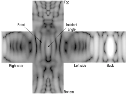
As a comparison, the same RCS obtained with the Cubed Sphere sampling scheme is seen in Figure 5. This image illustrates the behavior of the RCS at the top and bottom more clearly. The different regions can be connected along each edge of every region. The right edge of the back region can be connected with the left edge of the right side and the right edge of the bottom region can be connected with the lower edge of the left side, etc.

The Conventional scattered bistatic RCS matrix of the F-117 model at 100 MHz is depicted in Figure 6 for an incident angle of 90 degrees in elevation and 0 degrees in azimuth. Thus, the incident aspect angle coincides with the longitudinal axis of the aircraft.

Figure 4. The monostatic RCS matrix of the F-117 model at 5 GHz and horizontal polarization sampled with the Conventional sampling scheme. The dynamic range is 150 dB.

Figure 5. The monostatic RCS matrix of the F-117 model at 5 GHz and horizontal polarization sampled with the Cubed Sphere sampling scheme. The dynamic range is 150 dB.

Figure 6. The scattered bistatic RCS of the F-117 model at 100 MHz and horizontal polarization with an incident angle of 90 deg. elevation and 0 degrees azimuth, sampled with the Conventional sampling scheme. The dynamic range is 50 dB.

Figure 7. The scattered bistatic RCS of the F-117 model at 100 MHz and horizontal polarization with an incident angle of 90 deg. elevation and 0 degrees azimuth, sampled with the Cubed Sphere sampling scheme. The dynamic range is 50 dB.

Figures 4–7 show the RCS calculated using the two sampling schemes and as expected it can be seen that the patterns are similar. However, the figures do not reveal which scheme that offers the best modeling accuracy.

It was found that with an equal equatorial resolution the Cubed Sphere only required close to 75% of the samples for resolutions above one sample per degree in the monostatic case, and consequently 56% percent in the bistatic case.

Figure 8. Box and whisker plots of the relative interpolation error for samples with an equatorial resolution of 0.1 degree for the monostatic RCS. The dashed center-line is the median value of the relative interpolation error in Rmax; the bottom and top lines of the boxes correspond to the first and third quartile respectively. Values larger or smaller than 1.5 times the IQD beyond each quartile were considered outliers; this is represented by the length of the whiskers.

Figure 9. A comparison of interpolation accuracy as a function of the number of samples for the monostatic RCS at 5 GHz.

angular resolution, generated during this work, it was found that the median value approached zero as the number of evaluation samples increased. Therefore, the IQD alone can be a good measure of merit for different sampling schemes.

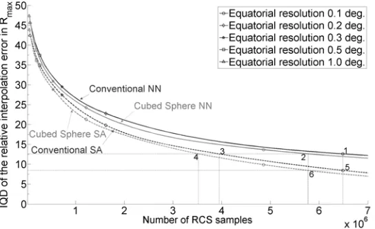
Figure 9 shows the IQD as a function of the number of samples required by each sampling scheme. This is a more reasonable comparison of sampling schemes because it shows how many samples are required to achieve certain interpolation accuracy for each scheme.

The markers indicate the equatorial angular resolution in the Conventional sampling scheme and the numbers and straight dashed lines in the figure are plotted to assist interpretation of the graph. Starting at 1, in Figure 9, it can be seen that if 6.5 million samples are taken with the Conventional scheme, and interpolated using NN, an IQD of 12.5 percent is obtained.

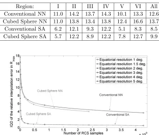
Figure 10. A comparison of interpolation accuracy as a function of the number of samples for the bistatic RCS at 100 MHz.

percent, without any loss of interpolation accuracy in the monostatic case. Going from 1 to 5 it can be seen that the IQD decreases from 12.5 to 8.5 percent by interpolating the Conventional sampling scheme with the SA instead of NN. The same IQD can be obtained with the Cubed Sphere sampling scheme using the SA, then the number of samples can also be decreased by about 0.7 million samples. In Table 1 the IQD for the monostatic interpolation at 5 GHz has been listed for the different regions of the Cubed Sphere sampling scheme and compared to the Conventional sampling scheme. The table reveals that, in regions I–IV the IQD of the cubed sphere is slightly lower compared to that of the Conventional scheme. In regions V–VI the IQD is 2–4 percentage points higher for the Cubed Sphere sampling scheme.

For the bistatic interpolation in Figure 10 it can be seen that the number of samples can be reduced substantially by using the Cubed Sphere sampling scheme instead of the Conventional sampling scheme when interpolating using NN. However, the SA seems to provide the same interpolation accuracy independently of the sampling scheme used.

4. DISCUSSION

A list of desirable properties for sampling schemes was given in the introduction. Each item on that list is addressed below, in light of the work presented.

1. The Cubed Sphere sampling scheme outperforms the Conventional sampling scheme when using the NN in terms of RCS accuracy per sample, in both the monostatic and bistatic evaluations; this can be seen in Figure 9 and Figure 10.

3. The Cubed Sphere sampling scheme can increase the resolution in certain regions, while confining the increased number of samples to one side of the cube. By comparison, refining the resolution in a certain region in the Conventional sampling scheme affects the entire domain.

4. The fact that the Conventional sampling scheme is stored in a structure consisting of a single RCS matrix, without any transformations, makes it more intuitive. However, by plotting the six sub-matrices of the Cubed Sphere sampling scheme, as seen in Figures 5 and 7, a better image of the complete RCS can be generated.

5. The Cubed Sphere scheme will inevitably introduce complications to regular measurement setups, which is not the case in the Conventional sampling scheme. Thus, there is a trade-off between time spent on setting up the sampling scheme and the time it takes to generate a sample.

In the work presented only one target is considered at two different carrier frequencies. Future studies could consider different kinds of targets; both simple and complex targets should be of interest. However, the aim of this study was to present and evaluate the idea of using the Cubed Sphere for sampling RCS data. For this purpose one complex target should be sufficient as a demonstrator and it is very likely that the benefits presented will also apply to other targets.

The IQD was herein used as a measure of merit for interpolation of RCS data. This is a good candidate for measuring the variability in the accuracy, since it is straightforward to interpret its meaning, since it can be related to operational demands on the platform for which the RCS is analyzed. Table 1 shows that the Conventional sampling scheme has higher interpolation accuracy around the poles, where the sampling density is higher, and performs similar to the Cubed Sphere sampling scheme around the equator. When sampling over the entire domain it is desirable to have a similar resolution over the entire domain; this is achieved by the Cubed Sphere sampling scheme.

In this work, the number of samples taken is much higher than what is realistic in any measurement setup; however, the number of samples can be reduced by 25% at an equatorial resolution of one degree in the monostatic case. This comes with the price of lower interpolation accuracy, especially at the poles. However, since measurements are often expensive and time consuming, it should be worth considering the Cubed Sphere sampling scheme.

5. CONCLUSIONS

By using the Cubed Sphere sampling scheme in RCS measurements and calculations it is possible to decrease the number of samples required by approximately 25% for the same equatorial resolution when sampling monostatic RCS data.

It has been shown that, without any loss in accuracy, the number of samples can be reduced significantly when sampling RCS data over the entire domain by using the Cubed Sphere sampling scheme and interpolating with the SA. If properly implemented, alternative sampling schemes can greatly reduce costs in terms of both time and money spent on electromagnetic computations and measurements.

ACKNOWLEDGMENT

This work was supported in part by the Swedish innovation agency VINNOVA. (Contract No. 2010-01259).

REFERENCES

1. Sinclair, G., “Early history of the OSU ElectroScience Laboratory,” IEEE Transactions on Antennas and Propagation, Vol. 33, No. 2, 137–143, Feb. 1985, DOI: 10.1109/TAP.1985.1143545. 2. Dybdal, R. B., “Radar cross section measurements,” Proceedings of the IEEE, Vol. 75, No. 4,

498–516, Apr. 1987.

and Propagation Magazine, Vol. 56, No. 4, 34–43, Aug. 2014, DOI: 10.1109/MAP.2014.6931656. 10. Yang, J. and K. T. Sarkar, “Interpolation/Extrapolation of Radar Cross-Section (RCS) data in the

frequency domain using the cauchy method,” IEEE Transactions on Antennas and Propagation, Vol. 55, 2844–2851, Oct. 2007.

11. Davis, M. E., “Space based radar moving target detection challenges,” RADAR, 143–147, 2002. 12. Manasse, R., “Idealized radar GMTI detection with space-time processing,” IEEE Transactions

on Aerospace and Electronic Systems, Vol. 45, No. 4, 1610–1618, Oct. 2009, DOI:

10.1109/TAES.2009.5310322.

13. Li, J., G. Liu, N. Jiang, and P. Stoica, “Moving target feature extraction for airborne high-range resolution phased-array radar,” IEEE Transactions on Signal Processing, Vol. 49, No. 2, 277–289, Feb. 2001, DOI: 10.1109/78.902110.

14. Wang, Y. L., Z. Bao, and Y. N. Peng, “STAP with medium PRF mode for non-side-looking airborne radar,”IEEE Transactions on Aerospace and Electronic Systems, Vol. 36, No. 2, 609–620, Apr. 2000, DOI: 10.1109/7.845249.

15. Ulander, L., P. F¨orlind, P. Grahn, and A. Gustavsson, “Bistatisk och passiv radar,” FOI, Stockholm, 2014.

16. Amanipour, V. and A. Olfat, “CFAR detection for multistatic radar,”Signal Processing, Vol. 91, No. 1, 28–37, Jan. 2011, DOI: 10.1016/j.sigpro.2010.06.003.

17. Willis, N. J. and G. Griffiths, Advances in Bistatic Radar, 91–104, SciTech Publishing, Raleigh, 2007.

18. Ronchi, C., R. Iacono, and P. S. Paolucci, “The ‘cubed sphere’: A new method for the solution of partial differential equations in spherical geometry,” Journal of Computational Physics, Vol. 124, No. 1, 93–114, Mar. 1996, DOI: 10.1006/jcph.1996.0047.

19. Hiroyuki, A. and I. Nozomu, “Sampling points reduction in spherical scanned TRP,” IEEE Conference on Antenna Measurements & Applications, 1–4, 2014.

20. Cornelius, R. and D. Heberling, “Analysis of sampling grids for spherical near-field antenna measurements,” PIERS Proceedings, 923–927, Prague, Jul. 6–9, 2015.

21. Giordanengo, G., M. Righero, F. Vipiana, G. Vecchi, and M. Sabbadini, “Fast antenna testing with reduced near field sampling,” IEEE Transactions on Antennas and Propagation, Vol. 62, No. 5, 2501–2513, May 2014, DOI: 10.1109/TAP.2014.2309338.

22. Jenn, D. C., “POFACETS 4.1,” 2013, [Online], Available: http://faculty.nps.edu/jenn.

23. Van den Bosch, I., “Puma-EM 5.8,” 2014, [Online], Available: http://sourceforge.net/projects/ puma-em/.

24. Shaeffer, J. F., M. T. Tuley, and E. F. Knott,Radar Cross Section, 2nd Edition, 17, 44–45, Artech House Publishers, Norwood, 1993.

25. De Boor, C.,A Practical Guide to Splines, 291–296, Springer New York, New York, NY, 2001. 26. Marsaglia, G., “Choosing a point from the surface of a sphere,” The Annals of Mathematical