A Rank-
(L, L,
1)
BCD based AOA-Polarization Joint Estimation
Algorithm for Electromagnetic Vector Sensor Array
Yu-Fei Gao and Qun Wan*
Abstract—This paper investigates an angle of arrival (AOA) and polarization joint estimation
algorithm for an L-shaped electromagnetic vector sensor array based on rank-(L, L,1) block component decomposition (BCD) tensor modeling. The proposed algorithm can take full advantage of the multidimensional information of electromagnetic signal to obtain the parameter estimation more accurately than the matrix-based method and the existing tensor decomposition method. In addition, the algorithm can accomplish pair-matching of estimated parameters automatically. The numerical experiments demonstrate that even under the conditions of low SNR and limited snapshots, the proposed algorithm can still steadily achieve high detection probability with low estimation error, which is important for practical applications.
1. INTRODUCTION
Electromagnetic vector sensor (EMVS) is a kind of antenna element which can detect electromagnetic wave with different polarization forms and fully acquire information carried by the wave. Many researches have been presented to study the problem of parameter estimation of EMVS array [1–3]. However, the existing methods are based on vector or matrix modeling, which are inappropriated to the received signal of EMVS array with inherent multidimensional structure. Recently, tensor-based methods have received attention in signal processing [4]. Compared with vector or matrix modeling, tensor modeling is more suitable to multidimensional signals [5, 6]. In the past decade, tensor decomposition has been widely applied to EMVS array signal processing [7–9]. However, the existing tensor-based methods for EMVS array are mostly based on canonical polyadic decomposition (CPD) model. This model has the advantage of decomposition uniqueness, but the decomposition factors must satisfy rank-1 condition, which may not be true in practice [10]. It is expected that a new tensor framework needs to be developed. In 2008, De Lathauwer proposed a tensor decomposition model, i.e., block component decomposition (BCD), which is able to overcome the shortcoming [11, 12]. The BCD-based tensor methods can not only maintain the uniqueness of decomposition, but also relax the requirement for rank constraint [13, 14]. To the best of our knowledge, there has been little public research on the application of BCD in EMVS array. Besides, the angle pair-matching is a challenging problem in parameter estimation for array signal processing. Since rank-(L, L,1) BCD method possesses a blind estimation feature, it can solve such a problem suitably. Motivated by the background above, this paper proposes a rank-(L, L,1) BCD-based parameter estimation algorithm for EMVS array.
The rest of this paper is organized as follows. Section 2 describes the received signal model of EMVS array based on rank-(L, L,1) BCD modeling. Section 3 develops the AOA-polarization estimation algorithm. Section 4 presents numerical simulations to verify the proposed algorithm. The last section concludes this paper.
Received 8 February 2017, Accepted 28 March 2017, Scheduled 16 April 2017 * Corresponding author: Qun Wan ([email protected]).
2. RANK-(L, L,1) BCD MODELING FOR EMVS ARRAY
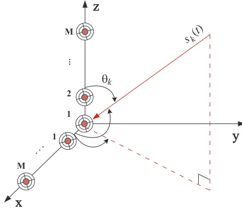
This paper adopts an L-shaped EMVS array [15], as shown in Fig. 1, which consists of a couple of orthogonal uniform linear arrays (ULA), and each hasM sensors. For partially polarized electromagnetic waves [1, 2], the received signal model can be expressed as
x(t) = (AxB)sT (t) +nx(t), (1)
z(t) = (AzB)sT (t) +nz(t), (2) where denotes the Khatri-Rao product [4]; Ax = [ax,1,ax,2, . . . ,ax,K] ∈ CM×K is the steering
matrix of the subarray along x-axis, defining the spatial frequency αk = −2πdλ cosφk, where λ is
the wavelength of source signal and d the array element spatial interval. Then we have ax,k = [1, ejα1, ejα2, . . . , ej(M−1)αK]T. B = [b
1, . . . ,bK]∈ C6×K is the polarization steering matrix, in which
bk = Θkgk, Θk ∈ R6×2 is the orientation matrix depending on AOA, and gk = [cosγk,sinγkejηk]T is
the amplitude-phase vector, where γ ∈ [0, π/2] is the auxiliary polarization angle and η ∈ [−π, π] the polarization phase difference [3]. s(t)∈C1×K is the source signal vector andnx(t)∈CM×1 the additive
white Gaussian noise (AWGN) vector. The signal model of the subarray alongz-axis is consistent with the form ofx-axis. Without loss of generality, the argument tis omitted in the following discussions for simplicity.
z
x
y
k
...
1
1 2 M
M
θ
s k(t)
Figure 1. L-shaped array configuration of EMVS array.
Combining the measurement of both subarrays [2], the received signal model can be expressed as
y=
K
k=1
Ak⊗bk·sTk +n, (3)
the operator ⊗ denotes Kronecker product; Ak = blockdiag(ax,k,az,k), where blockdiag(·) denotes a
block diagonal matrix. For N snapshots, Eq. (3) can be written as
Y = (AbB)ST +N, (4)
where b denotes the Khatri-Rao product in block form [12]. A = [A1, . . . ,AK]; S = [S1, . . . ,SK],
Sk = [sTk(1), . . . ,sTk(N)]T. N is the corresponding AWGN matrix. Note that Eq. (4) is the
rank-(L, L,1) BCD model [11], where L = 2. In this paper, the calligraphic capital letter is utilized to indicate tensor data, then the received signal model can be rewritten as
Y =
K
k=1
SkATk
where Y ∈ CN×2M×6 is the received signal in tensor form, and the mode-1 matricization is Y, i.e.,
Y = [Y](1), in which mode is considered as the order of tensor data [4]. Based on EMVS array signal model, the decomposition uniqueness of Eq. (5) should be investigated.
Definition 1 Essentially unique for rank-(L, L,1) BCD
The rank-(L, L,1) BCD described in Eq. (5) is called essentially unique, if the factors {S,A,B}
satisfy the following conditions, 1. Sk and Ak can be post-multiplied by Γk and (ΓT
k)−1, respectively,
where Γk∈CL×L is a nonsingular matrix; 2. corresponding to condition 1, all factors can be arbitrarily scaled; meanwhile, their product remains unchanged.
As concluded in [11], the conditions of decomposition uniqueness can be derived as: I. min(N,2M) ≥ LK; II.B does not contain proportional columns. Considering the definition ofBdescribed in received signal model, condition II is satisfied. Since L = 2 in this paper, when K ≤ min(N,2M)/2 , the uniqueness of Eq. (5) will be valid.
3. AOA-POLARIZATION ESTIMATION ALGORITHM
Considering the rank-(L, L,1) BCD model in Eq. (5) with additive noise, the proposed algorithm acquires the estimation of factor matricesAandBfrom the received signalYand obtain the estimation of spatial frequency{αk}Kk=1 and polarization amplitude-phase vector {gk}Kk=1. This paper adopts the minimum mean square error (MMSE) criterion [12],
min ˆ
Ak,ˆbk
Y −Yˆ2
F , k= 1,2, . . . , K,
s.t. Yˆ=
K
k=1
ˆ
SkAˆTk
◦ˆb
k,
(6)
where · F denotes the Frobenius norm. To solve the above problems, the alternating least squares (ALS) is introduced [12, 16, 17]. With fixed two components ofS,A,Bin each iteration, the remaining one is updated by least squares approach, then the same scheme is repeated in turn until the convergence condition is satisfied.
For the array manifold configuration given in this paper,Ak can be parted asAk = [Ak,T1,ATk,2]T, where Ak,1 = [ax,k,0], Ak,2 = [0,az,k]. Because the BCD estimation result and steering matrix have
the same column space [11],Aˆk can be parted asAˆk= [AˆTk,1,AˆTk,2]T in the same way. Giving the SVD of{Aˆk,m}2m=1, i.e.,Aˆk,m=Uk,mΣk,mVk,mH , the left singular vectoruk,1 corresponding to the maximum singular value can be obtained. Take the first and last (M −1) rows of uk,1, denoted as ua and ub,
to construct Uab = [ua,ub]. Applying eigenvalue decomposition of UabHUab, i.e., UabHUab = WΛWH,
where
W =
w1,1 w1,2
w2,1 w2,2 ∈C
2×2
, (7)
yields the estimation of spacial frequency ˆαk = ∠(−ww12,,22), where ∠(·) denotes the phase angle of a
complex variable. Thus the estimation of the arrival angle on the array along x-axis can be obtained, ˆ
φk = arccos(−αˆkλ
2πd ). The same method can be used to get the estimation of the elevation angle ˆθk.
Then the azimuth angle φk can be estimated directly, ˆφk = arccos(
cos ˆφk
sin ˆθk). Since Aˆk includes the
steering vector information on both subarrays, and the type-2 BCD possesses the uniqueness [13], the estimations of azimuth and elevation angles accomplish the matching pairing automatically.
After obtaining the polarization steering matrix by ALS and the estimation of AOA, the polarization amplitude-phase vector can be obtained. Consider bk=Θkgk, where Θk is calculated by substituting
( ˆφk,θˆk), then we have gˆk = Θ†kˆbk. Consequently, the estimations of auxiliary polarization angle and
polarization phase difference are ⎧
⎨ ⎩
ˆ
γk = arctan
gˆk(2)
ˆ
gk(1)
ˆ
ηk=∠(ˆgk(2))
4. NUMERICAL EXPERIMENTS AND DISCUSSION
In this section, several numerical experiments are presented to verify the effectiveness of the proposed algorithm and compare its performance with the existing methods. It is assumed that the L-shaped array consists of two ULAs, and each has M sensors. The number of signals is K; the snapshots is N; the Monte-Carlo independent trials is L.
4.1. Implementations of AOA-Polarization Estimation
4.1.1. Different SNRs
The simulation parameters are set as: M = 5, K = 2, N = 200; the array element interval is λ2; two groups of AOAs are (φ1, θ1) = (100◦,65◦), (φ2, θ2) = (80◦,115◦), and the corresponding polarization parameters are (γ1, η1) = (25◦,−30◦), (γ2, η2) = (75◦,40◦). The SNR is set as −3 dB ∼ 15 dB and Monte-Carlo trialsL= 500. The AOA estimation results are shown in Fig. 2(a). The estimation results of auxiliary polarization angles and phase difference are shown in Fig. 2(b). The simulation results show that the higher precision of parameter estimation can be obtained by means of the algorithm proposed in this paper. Even under the situation of low SNR, the AOAs, auxiliary polarization angles and auxiliary polarization phase difference can still be fully distinguished, which demonstrates the anti-noise robustness of this algorithm.
75 80 85 90 95 100 105
60 70 80 90 100 110 120
Azimuth angle (deg)
Elevation angle (deg)
SNR = 3 dB SNR = 3 dB SNR = 9 dB SNR = 15 dB
20 40 60 80
-60 -40 -20 0 20 40 60 80 100
Auxiliary polarization angle (deg)
Polarization phase difference (deg)
SNR = 3 dB SNR = 3 dB SNR = 9 dB SNR = 15 dB
(a) (b)
Figure 2. AOA and polarization scatterplots under different SNRs, by 500 Monte-Carlo trials. (a)
(φ1, θ1) = (100◦,65◦), (φ2, θ2) = (80◦,115◦). (b) (γ1, η1) = (25◦,−30◦), (γ2, η2) = (75◦,40◦).
4.1.2. Different Snapshots
This group of simulations assign the snapshotsN ∈[5,1000]. The SNR is fixed at 5 dB. The remaining parameters are the same as those in Section 4.1.1. The simulation results of AOA are shown in Fig. 3(a). The results for the auxiliary polarization angles and phase difference can be seen in Fig. 3(b). The results indicate that the algorithm developed in this paper has higher angular resolution, even under the situation of limited snapshots.
4.2. Performance Comparison with Other Methods
80 85 90 95 100 60 70 80 90 100 110 120
Azimuth angle (deg)
Elevation angle (deg)
Snapshots = 20 Snapshots = 50 Snapshots = 200 Snapshots = 500 Snapshots = 1000
20 40 60 80
-60 -40 -20 0 20 40 60 80
Auxiliary polarization angle (deg)
Polarization phase difference (deg)
Snapshots = 20 Snapshots = 50 Snapshots = 200 Snapshots = 500 Snapshots = 1000
(a) (b)
Figure 3. AOA and polarization scatterplots under different snapshots, by 500 Monte-Carlo trials. (a)
(φ1, θ1) = (100◦,65◦), (φ2, θ2) = (80◦,115◦). (b) (γ1, η1) = (25◦,−30◦), (γ2, η2) = (75◦,40◦).
4.2.1. RMSE
We first investigate the RMSE which is defined as
1
L
L
l=1( φ(l)2+ θ(l)2+ γ(l)2+ η(l)2), where
φ(l) = K1
K
k=1|φˆk(l) − φk|, θ(l) = 1
K
K
k=1|θˆk(l) − θk|, γ(l) = 1
K
K
k=1|ˆγk(l) − γk| and
η(l) = K1
K
k=1|ˆηk(l) −ηk|, in which ˆφk(l),θˆk(l),γˆk(l),ηˆk(l) are the estimated values of the k-th group signal parameters at the l-th Monte-Carlo trial. The Cramer-Rao lower bound is defined as
1
K
K
k=1(CRB(φk) +CRB(θk) +CRB(γk) +CRB(ηk)), where CRB(φk), CRB(θk), CRB(γk) and
CRB(ηk) are the diagonal elements of CRB matrix [1, 7], corresponding to the parametersφk, θk, γk, ηk,
respectively. The RMSE curves versus SNRs and snapshots are shown in Fig. 4(a) and Fig. 4(b), respectively.
The simulation result in Fig. 4(a) reveals that RMSE of the proposed algorithm is always smaller than the reference methods within the entire SNR interval. The reason is that the tensor-based method takes full advantage of the multidimensional information of received signal. This inherent feature makes
-3 0 3 6 9 12 15
10 -1
SNR (dB) RMSE MUSIC CPD Proposed CRLB
5 20 50 100 200 300 500 1000 10 -1
Snapshots RMSE MUSIC CPD Proposed CRLB (a) (b)
Figure 4. RMSE comparison, by 500 Monte-Carlo trials. (a) Versus different SNRs. (b) Versus
the two tensor-based algorithms have a better estimation performance than the matrix-based subspace algorithms, e.g., MUSIC, which can only make use of one-dimensional information. So far as the comparison between the two tensor-based algorithms, the performance of BCD is better than CPD. As the analysis in Section 3, the former gives the united steering matrix Ak directly and finishes the pair matching of estimated parameters automatically.
The RMSE curves in Fig. 4(b) demonstrate that both the tensor-based methods are better than the classic subspace method with different snapshots. From the analysis in Section 4.2, the uniqueness condition of BCD modeling for EMVS array is min(N,2M)/2 ≥K. For this group of experiments, M = 5, K = 2. Consequently, the uniqueness condition is met so long as N > 4. Besides, according to the analysis results of the detection probability in Section 4.2.2, even with limited snapshots, BCD can still maintain a higher level of detection probability. This is a main reason of its better error performance than other reference methods.
4.2.2. Detection Probability
The detection probability represents the success rate of pair matching between the two groups of signal parameters for EMVS array. We compare the detection probabilities among three methods and carry out two groups of simulation experiments for different SNRs and snapshots, which are shown in Fig. 5(a) and Fig. 5(b), respectively.
3 0 3 6 9 12 15
0.7 0.75 0.8 0.85 0.9 0.95 1
SNR (dB)
Detection Probability
MUSIC CPD Proposed
5 20 50 100 200 300 500 1000 0.75
0.8 0.85 0.9 0.95 1
Snapshots
Detection Probability
MUSIC CPD Proposed
(a) (b)
Figure 5. Detection probability comparison, by 500 Monte-Carlo trials. (a) Versus different SNRs.
(b) Versus different snapshots.
The graph in Fig. 5(a) demonstrates that detection probability curves coincide gradually with the SNR increasing and split obviously apart as the SNR decreasing, which implies the performance difference between individual methods under low SNR conditions. The proposed algorithm gives the highest detection probability of all the three methods. For instance, when SNR =−3 dB, the detection probability of the proposed algorithm is 93%, which is increased by nearly 39% relative to the value (67%) of MUSIC algorithm and by nearly 16% relative to the value (80%) of CPD algorithm. This result should be attributed to that BCD algorithm can jointly estimate the steering vectors of the both subarrays and accomplish the pair matching automatically, which makes BCD possess a better estimation performance even under a severe noise situation.
of the reference methods are severely impacted by snapshots, e.g., the detection probability of MUSIC varies rapidly as the snapshots increases. In comparison, the impact of the snapshots is quite slight on the proposed algorithm for which the detection probability curve varies evenly throughout the entire snapshots interval. This feature implies that the algorithm is more suitable for the practical applications with real-time requirement.
5. CONCLUSION
In this paper, the BCD tensor modeling for parameter estimation of EMVS array is investigated. For the fully polarized signal, a rank-(L, L,1) BCD based algorithm is developed to achieve AOA-polarization joint estimation. This algorithm can make the most of the multidimensional information of the received signal and automatically accomplish pair-matching of estimated parameters. Two groups of numerical experiments are conducted to verify the effectiveness of the algorithm. The results show that both the estimation accuracy and detection probability of the proposed algorithm are superior to the subspace method and CPD method. The algorithm maintains robust performance under severe conditions such as low SNR or limited snapshots, which has significance in practice.
ACKNOWLEDGMENT
This work was supported in part by the National Natural Science Foundation of China under Grant U1533125 and National Science and Technology Major Project under Grant 2016ZX03001022.
REFERENCES
1. Nehorai, A. and E. Paldi, “Vector-sensor array processing for electromagnetic source localization,”
IEEE Trans. Signal Process., Vol. 42, No. 2, 376–398, Feb. 1994.
2. Tan, K.-C., K.-C. Ho, and A. Nehorai, “Linear independence of steering vectors of an electromagnetic vector sensor,”IEEE Trans. Signal Process., Vol. 44, No. 12, 3099–3107, Dec. 1996. 3. Wong, K. T. and M. D. Zoltowski, “Uni-vector-sensor esprit for multisource azimuth, elevation,
and polarization estimation,” IEEE Trans. Antennas Propag., Vol. 45, No. 10, 1467–1474, 1997. 4. Cichocki, A., D. Mandic, L. De Lathauwer, G. Zhou, Q. Zhao, C. Caiafa, and H. A. Phan, “Tensor
decompositions for signal processing applications: From two-way to multiway component analysis,”
IEEE Signal Process. Mag., Vol. 32, No. 2, 145–163, 2015.
5. Sidiropoulos, N. D., R. Bro, and G. B. Giannakis, “Parallel factor analysis in sensor array processing,” IEEE Trans. Signal Process., Vol. 48, No. 8, 2377–2388, 2000.
6. Gao, Y.-F., L. Zou, and Q. Wan, “A two-dimensional arrival angles estimation for L-shaped array based on tensor decomposition,” AEU Int. J. Electron. Commun., Vol. 69, No. 4, 736–744, 2015. 7. Miron, S., X. Guo, and D. Brie, “DOA estimation for polarized sources on a vector-sensor array
by parafac decomposition of the fourth-order covariance tensor,”16th European Signal Processing Conference, 1–5, Aug. 2008.
8. Guo, X., S. Miron, D. Brie, S. Zhu, and X. Liao, “A candecomp/parafac perspective on uniqueness of DOA estimation using a vector sensor array,” IEEE Trans. Signal Process., Vol. 59, No. 7, 3475–3481, Jul. 2011.
9. Forster, P., G. Ginolhac, and M. Boizard, “Derivation of the theoretical performance of a tensor music algorithm,”Signal Process., Vol. 129, 97–105, 2016.
10. Stegeman, A., “Candecomp/Parafac: From diverging components to a decomposition in block terms,”SIAM J. Matrix Anal. Appl., Vol. 33, No. 2, 209–215, 2012.
11. De Lathauwer, L., “Decompositions of a higher-order tensor in block terms — Part ii: Definitions and uniqueness,”SIAM J. Matrix Anal. Appl., Vol. 30, No. 3, 1033–1066, 2008.
13. De Lathauwer, L., “Blind separation of exponential polynomials and the decomposition of a tensor in rank-(l r,l r,1) terms,”SIAM J. Matrix Anal. Appl., Vol. 32, No. 4, 1451–1474, 2011.
14. Zhao, Q., C. F. Caiafa, D. P. Mandic, Z. C. Chao, Y. Nagasaka, N. Fujii, L. Zhang, and A. Cichocki, “Higher order partial least squares (hopls): A generalized multilinear regression method,” IEEE Trans. Pattern Anal. Mach. Intell., Vol. 35, No. 7, 1660–1673, 2013.
15. Nie, X. and P. Wei, “Array aperture extension algorithm for 2-d DOA estimation with L-shaped array,”Progress In Electromagnetics Research Letters, Vol. 52, 63–69, 2015.
16. Comon, P., X. Luciani, and A. L. De Almeida, “Tensor decompositions, alternating least squares and other tales,” J. Chemom., Vol. 23, No. 7–8, 393–405, 2009.
17. Sorber, L., M. Van Barel, and L. De Lathauwer, “Optimization-based algorithms for tensor decompositions: Canonical polyadic decomposition, decomposition in rank-(l r,l r,1) terms, and a new generalization,” SIAM J. Optim., Vol. 23, No. 2, 695–720, 2013.
18. Miron, S., N. Le Bihan, and J. I. Mars, “Vector-sensor music for polarized seismic sources localization,”EURASIP J. Adv. Signal Process., Vol. 2005, No. 1, 1–11, 2005.
19. Zhang, X. and D. Xu, “Deterministic blind beamforming for electromagnetic vector sensor array,”