Analysis of Scattering from Composite Conductor and Dielectric
Objects Using Single Integral Equation Method
and MLFMA Based on JMCFIE
Hua-Long Sun*, Chuang-Ming Tong, and Peng Peng
Abstract—A highly efficient hybrid method of single integral equation (SIE) and electric/magnetic current combined field integral equation (JMCFIE) is presented, named as SJMCFIE, for analysing scattering from composite conductor and dielectric objects, in which, SIE can reduce one half unknowns in dielectric region. The resultant matrix equation of SJMCFIE can be represented in the iteration form, which makes the computation complexity reduced further, and coupling mechanism of composite model becomes more explicit. For accelerating matrix-vector multiplications (MVMs), Multilevel Fast Multipole Algorithm (MLFMA) is employed to combine SJMCFIE to formulate SJMCFIE-MLFMA at last, which is the extension of SIE-MLFMA in the proposed reference. Finally, some examples verify the new hybrid method on accuracy, memory storage, computation efficiency compared to SIE-MLFMA and JMCFIE-MLFMA. Besides, SJMCFIE-MLFMA can also be used to analyse the complete coated model’s scattering.
1. INTRODUCTION
Analyzing electromagnetic scattering from composite conductor and dielectric objects has gained wide interest from many researchers, which have the importance in studying coated targets, cavity filled with dielectric materials, printed antenna on substrate, and substrate integrated waveguide (SIW). Specially, the research on stealthy weapon platforms and system, and the target’s recognition motivates the requirement for precisely computing and analyzing the target’s electromagnetic scattering. Traditional high-frequency asymptotic methods are not suitable for this kind of requirement due to poor accuracy in spatial, angular and frequency domain, whereas numerical algorithms are suitable for this situation due to their high precision. Computing composite models can utilize the methods based on surface integral equation [1–4], hybrid volume-surface integral equations [5], or Finite-Element-Boundary-integral techniques [6]. The methods based on surface integral equation have the advantage over hybrid volume-surface integral equation on computing homogeneous material objects. In practice, when analyzing scattering from composite objects based on surface integral equations, the conducting part usually utilizes electric field integral equation (EFIE), magnetic field integral equation or combined field integral equation, and the dielectric part utilizes Poggio-Miller-Chang-Harrington-Wu-Tsai (PMCHWT) equations [7], electric and magnetic current combine field integral equation (JMCFIE) [8–12], or N-M¨uller integral equations [13]. Especially, formulating equations in the dielectric part concerns both equivalent electric and magnetic currents. Yeung [14] proposes single integral equation (SIE), which only concerns the effective currents rather than both electric and magnetic currents, and as a result, the unknowns of SIE are only one half of JMCFIE or PMCHWT. However, SIE in [14] is only used to analyze the pure dielectric objects. Then, Wang et al. [15] extend SIE to analyze the combined conducting and
Received 13 August 2016, Accepted 12 November 2016, Scheduled 6 December 2016
* Corresponding author: Hua-Long Sun ([email protected]).
dielectric bodies, and incorporate multilevel fast multipole algorithm (MLFMA) [16, 17] as the extension of fast multipole method (FMM) [18] to reduce the complexity of matrix-vector products. It is worth to note that SIE-MLFMA in [15] is based on EFIE, so its iteration convergence is usually slower than that of magnetic field integral equation and magnetic field integral equation.
In this paper, a highly efficient hybrid method of SIE and JMCFIE is presented, named as SJMCFIE, to perform scattering from composite conductor and dielectric objects, which has two advantages: one is that JMCFIE guarantees fast convergence of iteratively solving compared to EFIE in SIE-MLFMA [15], and the other is that further SIE translates non-compact operators into compact operators [19–21] to achieve fast convergence of iteratively solving compared to JMCFIE. SJMCFIE can be rewritten in new iteration form, which not only reduces computation complexity, but also makes coupling mechanism explicit. With the unknowns of composite conductor and dielectric objects, solving resultant matrix equation based SJMCFIE gets harder. Like SIE-MLFMA, SJMCFIE-MLFMA is obtained by adopting MLFMA to accelerate MVMs. Examples show that: SJMCFIE-MLFMA has higher efficiency and accuracy than SIE-MLFMA and JMCFIE-MLFMA. Finally, SJMCFIE-MLFMA can also be used to analyze scattering from the complete coated model.
2. FORMULATION
2.1. Hybrid Method of SIE and JMCFIE
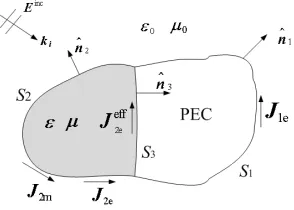
A typical model of composite conductor and dielectric objects is shown in Fig. 1. S1 and S2 are
the surfaces of the conductor and dielectric domain, respectively. S3 is the common interface of the
conductor and dielectric domain. J1e is induced electric current on the exterior surface S1, and J2e
and J2m are equivalent surface electric and magnetic currents on the exterior surface of S2. J2effe is
single effective current on the interior surface of the dielectric domain enclosed by S2 and S3. ε0 and
μ0 are the permittivity and permeability in the free space, respectively. ε and μ are the permittivity
and permeability in the dielectric region, respectively.
Figure 1. Illustration of composite conductor and dielectric objects illuminated by the incident.
Scattering field outside S1 and S2 can be computed by J1e located on the exterior surfaceS1, and J2e and J2m located on the exterior surface S2:
Es =η0L0(J1e) +η0L0(J2e)−K0(J2m) Hs=K0(J1e) + (1/η0)L0(J2m) +K0(J2e) (1)
where subscript 0 denotes the free space, and L0(·) and K0(·) are electric field integral operator and
magnetic field integral operator, respectively:
L0(f) = −jk0
Sm
[g0(r,r)f(r) + (1/k20)∇g0(r,r)∇·f(r)]dS m= 1,2 (2a)
K0(f) = −
Sm
[f(r)× ∇g0(r,r)]dS m= 1,2 (2b)
with g0(r,r) = exp(−jk0|r − r|)/(4π|r −r|) being the Green’s function in the free space and
η0 =
boundary condition of the JMCFIE formulation [4, 11]:
e1(r) =einc1 (r) +es1(r) = 0, j1(r) =jinc1 (r) +js1(r) =J1e, r∈S1
e2(r) =einc2 (r) +es2(r) =n2×J2m, j2(r) =jinc2 (r) +j2s(r) =J2e, r∈S2
, (3)
in which, e = n×E×n and j = n×H are the total tangential electric field and magnetic fields, respectively, andeinc(r) andjinc(r) are the incident wave’s tangential electric field and magnetic fields, respectively. Further, we have:
α η0
einc1 (r) +βjinc1 (r) =−αn1×L0(J1e)×n1−αn1×L0(J2e)×n1+(α/η0)n1×K˜0(J2m)×n1
+(β/2)J1e−βn1×K˜0(J1e)−(β/η0)n1×L0(J2m)−βn1×K˜0(J2e)r∈S1 (4a)
α η0
einc2 (r)+βjinc2 (r) =−αn2×L0(J1e)×n2−αn2×L0(J2e)×n2+
α 2η0
n2×J2m+
α η0
n2×K˜0(J2m)×n2
−βn2×K˜0(J1e)−(β/η0)n2×L0(J2m) + (β/2)J2e−βn2×K˜0(J2e)r∈S2 (4b)
with ˜K being the principle value integral, αand β the combination factors satisfying 0≤α,β≤1 and α+β= 1. The electric and magnetic currents are expanded with RWG function: J1e=
N1
j=1x1jf1j(r), J2e =
N2
j=1cjf2j(r) and J2m =
N2
j=1cjf2j(r), in which f1j and f2j are the RWG basis functions [22]
on S1 and S2, respectively. The total number of edges of S1 is N1, including the common edges [15]
connected toS1andS2, while the total number of edges ofS2isN2, excluding the common edges. In the
frame of Galerkin method, choose test function f1i and f2i for Equation (4) to formulate the resultant
matrix equation, simultaneously define the operator of two complex vectors as u, vΓ = Γu·vdΓ. Equations (4a) and (4b) can be translated into:
Q11
Q21
{x1}+
Q12 P12
Q22 P22
c d
=
b1
b2
, (5)
where
Qpp(i, j) = −αfpi, L0(fpj)Tpi+ (β/2)fpi,fpjTpi−β fpi,npi×K˜0(fpj)
Tpi
,
i, j∈[1, Np], p= 1,2, (6a)
Qpq(i, j) = −αfpi, L0(fqj)Tpi−β fpi,npi×K˜0(fqj)
Tpi
,
i∈[1, Np], j∈[1, Nq], {p, q}={1,2} ∪ {2,1}, (6b)
P12(i, j) = (α/η0) f1i,K˜0(f2j)
T1i−
(β/η0)f1i,n1i×L0(f2j)T1i,
i∈[1, N1], j∈[1, N2], (6c)
P22(i, j) =
α 2η0
f2i×n2i,f2jT2i+ (α/η0) f2i,K˜0(f2j)
T2i−
(β/η0)f2i,n2i×L0(f2j)T2i,
i, j∈[1, N2], (6d)
bp(i) = (α/η0)
fpi,Eincp
Tpi+β
fpi,n2i×Hincp
Tpi,
i∈[1, Np], p= 1,2. (6e)
The resultant matrix Equation (5) has the size of (N1+N2)×(N1+2N2) which is not sufficient for the
In SJMCFIE method, the fields in the dielectric domain can be computed with effective currentJ2effe on interior surface Sd= S2+S3, with the expression of Ed =η1L1(Jeff2e),Hd =K1(Jeff2e). η1 =
μ/ε being the wave impedance. Besides, inL1(·),K1(·) andg(r,r), wave number isk=w√με. It is pointed
out that the field represented by the effective currents satisfies the interior boundary condition onS2:
J2e=n2×Hd=−Jeff2e/2 +n2×K˜1(Jeff2e)
−J2m=n2×Ed=n2×η1L1(Jeff2e)
onS2 (7a)
and the boundary condition on the common surfaceS3 of the dielectric and the conducting body:
−αn3×L1(Jeff2e)×n3−(β/2)J2effe −βn3×K˜1(Jeff2e) = 0 onS3, (7b)
where the effective current on S3 has degenerated to surface equivalent current. Total effective
currents on the dielectric object’s interior surface can be expanded by RWG functions as Jeff2e(r) =
N2
i=1x2if2i +
N3
i=1x3if3i with the number of unknown edges being N2 +N3. Among them, N3 is
the number of unknown edges on S3 including the common edges. Referring to [14], the expansion
coefficients can be approximated by the average values passing through the edges:
xpi= (1/lpi)
lpi
(ˆlpi×npi)·Jeff2edl, p= 2,3. (8)
Combining Equations (7a) and (8), expansion coefficients{c} and {d}in Eq. (5) can be expressed as:
{c}= [ ˜P22]{x2}+ [ ˜P23]{x3}, {d}= [ ˜Q22]{x2}+ [ ˜Q23]{x3}, {0}= [ ˜Q32]{x2}+ [ ˜Q33]{x3}. (9)
Here,{x2}and{x3}are the vectors of the expansion coefficients of single effective currents. In Eq. (9),
submatrices’ elements can be represented as:
˜
P22(i, j) = −(1/2)δij −
l2i
(ˆl2i/l2i)·K˜1(f2j)dl, i, j∈[1,N2] (10a)
˜
P23(i, j) = −
l2i
(ˆl2i/l2i)·K˜1(f3j)dl, i∈[1,N2], j∈[1,N3] (10b)
˜
Q2q(i, j) =
l2i
(η1/l2i)ˆl2i·L1(fqj)dl, i∈[1,N2], j∈[1,Nq], q= 2,3 (10c)
˜
Q32(i, j) = −αf3i, L1(f2j)T3i−β f3i,n3i×K˜1(f2j)
T3i
, i∈[1,N3], j∈[1,N2] (10d)
˜
Q33(i, j) = −αf3i, L1(f3j)T3i−(β/2)f3i,f3jT3i−β f3i,n3i×K˜1(f3j)
T3i
, i, j∈[1,N3], (10e)
where, ifi=j,δij = 1; else if i=j,δij = 0. By substituting Eq. (9) into Eq. (5), new resultant matrix equation is obtained:
A11 A12 A13
A21 A22 A23
0 A32 A33
x1
x2
x3
=
b
1
b2
0
, (11)
where
[A11] = [Q11], [A12] = [Q12]·[ ˜P22] + [P12]·[ ˜Q22], [A13] = [Q12]·[ ˜P23] + [P12]·[ ˜Q23],
[A21] = [Q21], [A22] = [Q22]·[ ˜P22] + [P22]·[ ˜Q22], [A23] = [Q22]·[ ˜P23] + [P22]·[ ˜Q23],
[A32] = [ ˜Q32], [A33] = [ ˜Q33].
Due to adopting SIE, Equation (11) has the number of unknowns N1+N2+N3 less than one of
N1 + 2N2+N3 based on JMCFIE. We substitute x3 =−A−331A32x2 into Eq. (11), and a new matrix
equation is derived:
A11(A12−A13A−331A32)
A21(A22−A23A−331A32)
x1
x2
=
b1
b2
among which the number of unknowns N1+N2 is less than N1 +N2 +N3 in Eq. (11). A13A−331A32
represents indirectly mutual interaction between the dielectric exterior surface S2 and the conductor’s
exterior surfaceS1. A32 denotes the interaction betweenS2 and the common surface S3. A−331 denotes
the self-interaction of S3. A31 denotes the interaction between S1 and S3. In a word, the indirectly
mutual interaction’s process is S2→S3 →S1.
Similarly, A23A−331A32 indirectly represents self-interaction of the dielectric exterior surface S2,
which has the process of S2 →S3→S2.
When total number of unknowns is relatively low, directly solving Eq. (12) is enough; however, with number of unknowns getting higher, iterative solvers, such as Bi-Conjugate Gradients Stabilized Approach (BiCGSTAB) and Generalized Minimum Residual (GMRES) method [23], can effectively reduce the computation complexity. It is worth to note that during per iteration, A−331 concerns the matrix inversion, and in practice, we may translate A−331a= b into Ab33 =a, which can also be solved to achieve MVM A−331aby the iteration method. When N3 gets large, solving iteratively Ab33=a costs
more time, so Equation (11) is a better choice. Actually, SIE not only reduces the number of unknowns, but also improves the matrix condition number deduced from EFIE or combined field integral equation. As we know, matrix equation’s convergence performance is potentially determined by matrix condition number. Noticeably, magnetic field integral operator belongs to the second-kind Fredholm operator or compact operator, whereas electric field integral operator belongs to the first-kind Fredholm operator or compact operator [20]. Compact operator makes the matrix condition number better than non-compact operator because the former is well conditioned. JMCFIE includes non-non-compact operator or electric field integral operator in the dielectric domain that will worsen its matrix condition number, whereas SJMCFIE includes two-fold operators in the dielectric domain such as L0·K˜1, ˜K0·L1,L0·L1.
The multiplication of compact and non-compact operators is still a compact operator [20, 21], so the two former ones are compact operators. And the third term is the multiplication of two non-compact operators and is also a compact operator [13]. As a result, SJMCFIE improves matrix condition number in the dielectric domain. Iteration convergence will be improved and iteration steps reduced if adopting iteration methods for solving the resultant matrix equation. This conclusion has been numerically validated by Yeung in [14] when solving scattering from the pure dielectric object. Wang et al. attempt to incorporate SIE with EFIE, and as a result, the process of translating non-compact operator is similar to that in SJMCFIE. However, the conducting part is still based on EFIE, and obviously, this makes iteration convergence slow compared to combined field integral equation in SJMCFIE. Finally, the formulating process of resultant matrix equation in JMCFIE will cost more time than that in SJMCFIE, which will be verified in Section 3.
2.2. Formulation of SJMCFIE-MLFMA
At some level, utilizing the addition theorem [17], Green’s function and its Gradient can be expanded with the form of
e−jk0rij/r
ij = −j(k0/4π)
SE
d2keˆ −jk·(rim−rjm)T
0(k,rˆmm) (13a)
∇(e−jk0rij/r
ij) = −[k02/(4π)]
SE
ˆ
kd2keˆ −jk·(rim−rjm)T0(k,rˆmm) (13b)
where
T0(k,rˆmm) =
L l=0(−j)
l(2l+ 1)h(2)
l (k0rmm)Pl(ˆk·rˆmm).
Here,ri is a field point locating inm-th group with the centerrm, andrj is a source point locating inm-th group with the centerrm, satisfyingrim= ri− rm,rjm = rj− rm and rmm = rm− rm. SE stands for the Ewald spherical surface [24], and ˆkis the unit angular direction, k=k0ˆk. h(2)l is the
Hankel function of the 2nd kind. Pl is the Legendre polynomial. Lis the number of modes referring to [16]. Substituting Eq. (13) into Eq. (6), the well-separated group’s impedances can be approximated as
Qpq(i, j) =
SE
d2kUˆ imQpp·T0(k,rˆmm)VjmQqq , p, q= 1,2
Ppq(i, j) =
SE
d2ˆkUimPpp·T0(k,rˆmm)VjmPqq, p= 1,2; q= 2
UimQpp= [k20/(16π2)][α
Tpi
dse−jk·rimf
pi·( ¯I¯−kˆˆk) +βˆk×
Tpi
dse−jk·rim(n
pi×fpi)], p= 1,2
UimPpp= [k20/(16π2η0)][α
Tpi
ds(ˆk×fpi)e−jk·rim+β
Tpi
dse−jk·rim(f
pi×npi)·( ¯I¯−kˆk)],ˆ p= 1,2
VjmQqq =VjmPqq =
Tqj
dsejk·rjmf
qj·( ¯I¯−kˆk),ˆ q = 1,2
(14)
However, for Equation (9), wave number, wave impedance and Green’s function should be replaced with k, η1 and g with respect to ε, μ in the dielectric region. So in Equation (9), the well-separated
group’s impedances can be approximated as
˜
P2q(i, j) =
SE
d2kUˆ imP˜22·T1(k1,rˆmm)V ˜ Pqq
jm, q= 2,3
˜
Q2q(i, j) =
SE
d2ˆkUimQ˜22·T1(k1,rˆmm)V ˜ Qqq
jm , q = 2,3
˜
Q3q(i, j) =
SE
d2ˆkUimQ˜33·T1(k1,rˆmm)V ˜ Qqq
jm , q = 2,3
UimP˜22 = [k2/(l2i16π2)]
l2i
dl(ˆl2i׈k)e−jk1·rim,
UimQ˜22 =−[(η1k2)/(l2i16π2)]
l2i
dle−jk1·riml2
i·( ¯I¯−ˆkˆk),
UimQ˜33 = [k2/(16π2)]
α
Tpi
dse−jk1·rimf3i·( ¯I¯−ˆkˆk) +βˆk×
Tpi
dse−jk1·rim(n3i×f3i)
,
VP˜qq
jm =V ˜ Qqq jm =
Tqj
dsejk1·rjmfqj·( ¯I¯−kˆk),ˆ q = 2,3
in which,k1=kˆk, andUim,Vjm andT0/T1 are the receiving pattern, radiation pattern and translation
pattern respectively. Substituting Eqs. (14) and (15) into Eqs. (5) and (9), we have:
Qpq=Qnearpq + Lf
l=2
UQ(lpp) T0(l)VQ(lqq), p, q= 1,2
Ppq =Ppqnear+
Lf
l=2
UP(lpp)T0(l)VP(qql), p, q= 1,2
˜
P2q= ˜P2nearq + Lf
l=2
U(˜l)
P22T (l) 1 V
(l) ˜
Pqq, q = 2,3
˜
Q2q= ˜Qnear2q + Lf
l=2
U(˜l)
Q22T (l) 1 V
(l) ˜
Qqq, q= 2,3
˜
Q3q= ˜Qnear3q + Lf
l=2
U(˜l)
Q33T (l) 1 V
(l) ˜
Qqq, q= 2,3
(16)
Here, theLfth level is the finest level, andLf is the number of total levels. U(l),V(l) andT0(l)/T1(l) are the disaggregation, aggregation and translation matrices at the l-th level, respectively, in which U(l) and V(l) are composed of U
im and Vjm in Eqs. (14) and (15). The translation matrices at each
level, and aggregation and disaggregation matrices at the finest level may be precomputed and stored, which can utilize the symmetry of unit angular directions k to optimize storage requirement. As we know, MLFMA is used to accelerate MVMs per iteration and usually includes two sweeps: during the first sweep, the main implementation concerns the aggregation and translation processes. In detail, different from computing the aggregation matrices at the finest level, at the other levels the aggregation ones are indirectly computed by interpolation level-by-level from the (Lf −1)-th level to the second level. Simultaneously, the translation process about the well-separated groups is also done with the above aggregation process. During the second sweep, the incoming waves composed of aggregation and translation matrices’ elements with respect to some receiving group are computed level-by-level from the second level to the finest level by shifting and anterpolation [17]. After the above two sweeps, multiplying incoming waves by disaggregation matrices’ elements realizes the reduction of MVMs’ complexity in the resultant matrix Equation (12).
If adopting iteration method to solving Equation (11), the cost of one MVM in SJMCFIE is (N1+N2+N3)2, and for JMCFIE, the cost of one MVM is (N1+N2)2+(N1+N2)N2 on the exterior
surfaces ofS1 and S2, and is (N2+N3)2+ (N2+N3)N2 on S3 and interior surface ofS2, so the whole
cost of one MVM in JMCFIE is (N1+N2)2+ (N2+N3)2+ (N1+ 2N2+N3)N2. Obviously, SJMCFIE
has lower cost of one MVM than JMCFIE. Furthermore, because the condition number of SJMCFIE is better than that of JMCFIE as shown in Subsection 2.1, SJMCFIE has faster convergence property than JMCFIE. When combining MLFMA with SJMCFIE, redundant computations concerning sub-matrices’ MVMs will emerge and can be reduced. In detail, [Q11]{x1} and [Q21]{x1} have the same aggregation
terms for Equation (11). This property is also reflected in [ ˜P22]{x2}, [ ˜Q22]{x2}and [ ˜Q32]{x2}, as well as
[ ˜P23]{x3}, [ ˜Q23]{x3} and [ ˜Q33]{x3}. After setting {y}= [ ˜P22]{x2},{y} = [ ˜Q22]{x2},{z}= [ ˜P23]{x3},
{z}= [ ˜Q23]{x3}, the property of having the same aggregation terms is also reflected in [Q12]{y} and
[Q22]{y}, [P12]{y} and [P22]{y}, [Q12]{z} and [Q22]{z}, [P12]{z} and [P22]{z}, respectively. So the
cost of one MVM is O((N1 +N2) log(N1 +N2)) on the exterior surfaces of S1 and S2 and on the
exterior surfaces ofS1 and S2 on composite objects’ exterior surface, and the cost of one MVM reaches
O((N2+N3) log(N2+N3)) onS3 and interior surface ofS2, so SJMCFIE-MLFMA has the computation
complexity of O((N1+N2) log(N1+N2) + (N2+N3) log(N2+N3)). Similarly, for JMCFIE-MLFMA,
the cost of one MVM is O((N1 + 2N2) log(N1 + 2N2)) on the exterior surfaces of S1 and S2 and is
O((2N2+N3) log(2N2 +N3)) on S3 and interior surface of S2, so it has the computation complexity
of O((N1 + 2N2) log(N1+ 2N2) + (2N2+N3) log(2N2 +N3)). Obviously, computation complexity of
As we see, hybrid method SJMCFIE-MLFMA is an extension of SIE-MLFMA in [15] due to (i) adopting JMCFIE rather than EFIE in SIE-MLFMA; (ii) Equation (12) explicitly reflecting coupling mechanism of the composite model; (iii) better condition number of resultant matrix. So the new hybrid method makes total computation more efficient than SIE-MLFMA.
3. NUMERICAL RESULTS AND DISCUSSION
3.1. A Composite Sphere
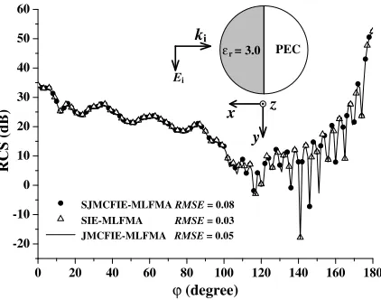
For verifying the validation of SJMCFIE-MLFMA, see a composite sphere composed of a perfecting conducting (PEC) hemisphere and a dielectric hemisphere with the relative permittivity εr = 3.0. The radius of this composite sphere is 6.0λ0 with λ0 the wavelength in free space. We have a total
of 102625 triangular patches with a length less than 0.09λ0 to model this composite sphere including
153938 unknowns if adopting SJMCFIE-MLFMA or SIE-MLFMA while 216175 unknowns have to be calculated if adopting JMCFIE-MLFMA.
For comparing the precision of these methods, define the root mean square error (RMSE) of
RMSE =
1
N
N
m=1
|RCSCalculated−RCSJMCFIE|2, (17)
whereN is the number of unknowns of the recorded azimuth.
Figure 2 shows the bistatic RCS of the composite sphere by SJMCFIE-MLFMA, SIE-MLFMA in [15] and JMCFIE-MLFMA. The parameters with respect to MLFMA haveDf = 0.2λ0,Lf = 6, and
L= 11 satisfying L=k0Df + 5 ln(π+k0Df) in outer domain of composite objects; Df = 0.2λwith λ
being the wavelength in dielectric part, Lf = 7, and L= 11 satisfying L=kDf + 5 ln(π+kDf) in the dielectric part. The computing platform is AMD processor of 2.3 GHz with 64 kernels and 64 GB RAM adopting Microsoft Visual C++ programming language. BICGSTAB is chosen as the iteration solver. Set relative error of unknown currents to be 10−5. Fig. 2 shows that the results by SJMCFIE-MLFMA and SIE-MLFMA are in good agreement with that by JMCFIE-MLFMA.
z x
y
PEC
εr= 3.0
Ei
ki
0 20 40 60 80 100 120 140 160 180 -20
-10 0 10 20 30 40 50 60
RCS (dB)
ϕ (degree)
SJMCFIE-MLFMA RMSE = 0.08 SIE-MLFMA RMSE = 0.03 JMCFIE-MLFMA RMSE = 0.05
Figure 2. The bistatic RCS curves of a composite sphere by three kinds of methods.
Also, Table 1 gives a detailed comparison of these three methods. JMCFIE-MLFMA costs more time in matrix filling process than SJMCFIE-MLFMA and SIE-MLFMA, because in the dielectric’s interior surface, the equation’s form of JMCFIE-MLFMA is similar to Equation (4). As a result, both of the electric and magnetic currents concern two integral operators L1(·) and K1(·) compared to the
single effective currents concerning L1(·) and K1(·). SIE-MLFMA and SJMCFIE-MLFMA have less
Table 1. Comparison of SIE-MLFMA, JMCFIE-MLFMA and SJMCFIE-MLFMA.
Matrix-filling time (s)
Storage requirement
(GB)
Computation time per iteration (s)
Iteration steps
Total computation
time (s)
SIE-MLFMA 203 5.862 5.3 224 1390.2
JMCFIE-MLFMA 369.8 8.152 7.8 120 1305.8
SJMCFIE-MLFMA 256 5.878 6.365 48 561.52
adopts EFIE, and the latter adopts CFIE. Due to better condition number of SJMCFIE, it needs the least iteration steps and total computation time.
3.2. A Bullet-shaped Composite Model
Another example is a bullet-shaped composite model illustrated in Fig. 3 including its geometric parameters. This model is composed of a conducting cylinder and coated head. The coated structure has the elliptical cross section with elliptical radii being a,b for the inner conductor and a1,b1 for the
outer coated layer.
z
x y
ki Ei
2
1 b
a
Unit: m b1
a1
Figure 3. The bullet-shaped composite model composed of the conducting cylinder and coated.
The working frequency is 2 GHz, and the incident wave illuminates the composite model with the incident angle θ = 0◦ and the polarization direction along x-axis. Computing platform and iteration solver are similar to that in the above example. Set the length of discretized patches to less than 0.09λ0,
0.05λ0, 0.03λ0 for the coated layer’s permittivity εr = 3.0, 5.0, 8.0, respectively. Fig. 4(a) gives the
bistatic RCS curves with different coated materials, while the coated structure hasa= 0.4 m,b= 0.9 m, and the thickness hast= (a1−a) = (b1−b) = 0.1 m. The parameters with respect to MLFMA satisfy
Df = 0.2λ0 andLf = 7,L= 11 in outer domain of composite objects. In the coated head’s domain, set
λto be the wavelength in dielectric part, and if relative permittivity has εr = 3.0, the coated domain hasDf = 0.2λ,Lf = 6,L= 11; if relative permittivity hasεr= 5.0, the coated domain hasDf = 0.24λ, Lf = 6,L= 12; if relative permittivity hasεr= 8.0, the coated domain hasDf = 0.2λ,Lf = 7,L= 11. The bistatic RCS curves are located on thex-z plane. Fig. 4(a) indicates that in total, with the coated material’s relative permittivity getting small, backscattering will decrease.
Figure 4(b) gives the bistatic RCS curves of the bullet-shaped composite model with different coated layer thicknesses t. The working frequency and cylinder part’s geometric parameter are similar to that in Fig. 3. The coated material has the relative permittivity εr = 5.0, and coated layer has the
maximum patch’s length of 0.05λ0. Set a1 = 0.5 m,b1 = 1 m. The parameters with respect to MLFMA
satisfyDf = 0.2λ0 and Lf = 7, L= 11 in outer domain of composite objects, and Df = 0.24λwith λ
being the wavelength in dielectric part, Lf = 6, L = 12 in the coated material’s domain. The bistatic
(a) (b)
Figure 4. The bistatic RCS curves of the bullet-shaped composite model with different coated layer material and thickness.
z y
x Ei
ki a b
Figure 5. The bistatic RCS curves of the coated cube with different coated layer’s thickness and relative permittivity.
that of t= 0 andt= 0.1 m. This example indicates that under the special condition, the coated layer thickness increases, and the backward RCS of the bullet-shaped composite model will increase.
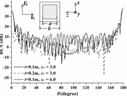
3.3. The Coated Object
Another typical composite model is the coated cube. It can also be computed by SJMCFIE-MLFMA, except that S1 does not exist. Equation (11) can be reduced to the form of
A22 A23
A32 A33
x2
x3
=
b2
0
, (18)
The inner conducting cube’s lengthaequals 1.5 m, and the coated layer’s thickness ist= (b−a)/2. Set the working frequency as 2 GHz, the incident direction as θ = 0◦, ϕ = 0◦, and scattering curves located on the x-z plane.
Figure 5 gives the comparison of different coated layer’s thicknesses and relative permittivities. Suppose that the maximum patch length is 0.09λ0 with coated material’s permittivity εr = 3.0. The
maximum patch length is 0.04λ0 with coated material’s permittivity εr = 6.0. When t = 0.1 m, the
coated object, are Df = 0.2λ, Lf = 7 and L = 11 in the interior domain of the coated material with
εr = 3.0, and are Df = 0.22λ, Lf = 7 andL = 11 in the interior domain of the coated material with εr= 6.0. Whent= 0.2 m, the parameters with respect to MLFMA areDf = 0.2λ0,Lf = 6 andL= 11
in the outer domain of the coated object, are Df = 0.2λ, Lf = 7 and L = 11 in the interior domain of the coated material with εr = 3.0, and are Df = 0.2λ, Lf = 8 and L = 11 in the interior domain of the coated material with εr = 6.0. As depicted in Fig. 5, under the condition of the same relative permittivity, scattering in almost all the directions will decrease with the thickness increasing, and under the condition of the same thickness, backscattering in directions ranging from 50◦ to 90◦ will decrease with the relative permittivity decreasing. This example illuminates that SJMCFIE-MLFMA can be applied in designing the coated layer to change the distribution of scattering energy. Simultaneously, due to this hybrid method’s high efficiency and accuracy, it can be incorporated with fast frequency or angular sweeping techniques to reduce the complexity in computing frequency or angular response.
4. CONCLUSION
This paper proposes a highly efficient hybrid method of SJMCFIE-MLFMA by combining SIE and MLFMA based on JMCFIE for computing composite conductor and dielectric objects. More details about formulating SJMCFIE-MLFMA are shown including the formulation of SJMCFIE and how to combine MLFMA with SJMCFIE. The final resultant matrix equation has fewer unknowns than that by JMCFIE, and this hybrid method based on JMCFIE is an extension of SIE-MLFMA based EFIE in the proposed reference, therefore has higher efficiency than SIE-MLFMA. Examples verify the accuracy and efficiency of this new hybrid method in computing composite models. Due to high efficiency and accuracy in computing composite conductor and dielectric objects, this hybrid method can be used in designing a local coated structure to effectively reduce backscattering. Besides, SJMCFIE-MLFMA also can be used in analyzing scattering from the complete coated model. This paper indicates that the scheme of combining SIE with MLFMA based on JMCFIE is feasible in analyzing scattering from the composite model composed of a single conductor and a single dielectric body. In the following, we focus on extending SJMCFIE-MLFMA to compute more complicated composite models composed of multi-objects with different dielectric materials.
ACKNOWLEDGMENT
The authors thank the National Natural Science Foundation of China (Grant No. 61372033).
REFERENCES
1. Harrington, R. F., Field Computation by Moment Methods, Oxford University Press, Oxford, England, 1996.
2. Peterson, A. and R. Mittra, “Convergence of the conjugate gradient method when applied to matrix equaitions representing electromagnetic scattering problems,” IEEE Trans. Antennas Propag., Vol. 34, No. 12, 1447–1454, 1986.
3. Volakis, J. L. and K. Sertel, Integral Equation Methods for Electromagnetics, SciTech Publishing, Raleigh, NC, USA, 2012.
4. Yl¨a-Oijala, P. and M. Taskinen, “Application of combined field integral equation for electromagnetic scattering by dielectric and composite objects,” IEEE Trans. Antennas Propag., Vol. 53, No. 3, 1168–1173, 2005.
5. Ewe, W. B., L. W. Li, and M. S. Leong, “Fast solution of mixed dielectric/conducting scattering problem using volumesurface adaptive integral method,” IEEE Trans.Antennas Propag., Vol. 46, No. 11, 3071–3077, 2004.
7. Yl¨a-Oijala, P., M. Taskinen, and S. J¨arvenp¨a¨a, “Analysis of surface integral equations in electromagnetic scattering and radiation problems,”Engineering Analysis with Boundary Elements, Vol. 32, 196209, 2008.
8. Donepudi, K. C., L. M. Jin, and W. C. Chew, “A higher order multilevel fast multipole algorithm for scattering from mixed conducting/dielectric bodies,” IEEE Trans. Antennas Propag., Vol. 2, No. 11, 2814–2821, 2002.
9. Yl¨a-Oijala, P., M. Taskinen, and J. Sarvas, “Surface integral equation method for general composite metallic and dielectric structures with junctions,” Progress In Electromagnetics Research, Vol. 52, 81–108, 2005.
10. Ubeda, E., J. M. Tamayo, and J. M. Rius, “Taylor-orthogonal basis functions for the discretization in method of moments of second kind integral equations in the scattering analysis of perfectly conducting or dielectric objects,”Progress In Electromagnetics Research, Vol. 119, 85–105, 2011. 11. Erg¨ul ¨O and L. G¨urel, “Fast and accurate analysis of large-scale composite structures with the
parallel multilevel fast multipole algorithm,” J. Opt. Soc. Amer. A, Vol. 30, No. 30, 509–517, 2013. 12. Lu, C. C. and Z. Y. Zeng, “Scattering and radiation modeling using hybrid integral approach and
mixed mesh element discretization,” PIERS Online, Vol. 1, 70–73, 2005.
13. Yl¨a-Oijala, P. and M. Taskinen, “Well-conditioned M¨uller formulation for electromagnetic scattering by dielectric objects,”IEEE Trans.Antennas Propag., Vol. 53, No. 10, 3316–3323, 2005. 14. Yeung, M. S., “Single integral equation for electromagnetic scattering by three-dimensional homogeneous dielectric objects,”IEEE Trans.Antennas Propag., Vol. 47, No. 10, 1615–1622, 1999. 15. Wang, P., M. Y. Xia, and L. Z. Zhou, “Analysis of scattering by composite conducting and dielectric bodies using the single integral equation method and multilevel fast multipole algorithm,”Microw.
and Opt.Tech.Lett., Vol. 48, No. 6, 1154–1156, 2006.
16. Song, J. M., C. C. Lu, and W. C. Chew, “Multilevel fast multipole algorithm for electromagnetic scattering by large complex objects,” IEEE Trans. Antennas Propag., Vol. 45, No. 10, 1488–1493, 1997.
17. Chew, W. C., J. M. Jin, E. Michielssen, and J. M. Song, Fast and Efficient Algorithms in Computational Electromagnetics, Artech House, Boston, MA, 2001.
18. Greengard, L. and V. Rokhlin, “A fast algorithm for particle simulations,” J. Comput. Phys., Vol. 73, 325–348, 1987.
19. Yan, S., J.-M. Jin, and Z. P. Nie, “Improving the accuracy of the second-kind Fredholm integral equations by using the Buffa-Christiansen functions,” IEEE Trans. Antennas Propag., Vol. 59, No. 4, 1299–1310, 2011.
20. Yan, S., J.-M. Jin, and Z. P. Nie, “A comparative study of Calderon preconditioners for PMCHWT equations,” IEEE Trans.Antennas Propag., Vol. 58, No. 7, 2375–2383, 2010.
21. Budko, N. V. and A. B. Samokhin, “Spectrum of the volume integral operator of electromagnetic scattering,”SIAM J.Sci.Comput., Vol. 28, No. 2, 682–700, 2005.
22. Rao, S. M., D. R. Wilton, and A. W. Glisson, “Electromagnetic scattering by surfaces of arbitrary shape,” IEEE Trans.Antennas Propag., Vol. 30, No. 3, 409–418, 1982.
23. Saad, Y.,Iterative Methods for Sparse Linear Systems, PWS Publishing Company, Boston, 1996. 24. Cui, T. J., W. C. Chew, G. Chen, and J. M. Song, “Efficient MLFMA, RPFMA, and FAFFA