Using High-Dimensional Color Transform To Detection Of Salient
Region Via Local Spatial Support
A Raghu Vardhan Babu
Abstract: In this paper, we introduce a novel approach to
automatically detect salient regions in an image. Our approach consists of global and local features, which complement each other to compute a saliency map. The first key idea of our work is to create a saliency map of an image by using a linear combination of colors in a high-dimensional color space. This is based on an observation that salient regions often have distinctive colors compared with backgrounds in human perception, however, human perception is complicated and highly nonlinear. By mapping the low-dimensional red, green, and blue color to a feature vector in a high-dimensional color space, we show that we can composite an accurate saliency map by finding the optimal linear combination of color coefficients in the high-dimensional color space. To further improve the performance of our saliency estimation, our second key idea is to utilize relative location and color contrast between superpixels as features and to resolve the saliency estimation from a trimap via a learning-based algorithm. The additional local features and learning-based algorithm complement the global estimation from the high-dimensional color transform-based algorithm. The experimental results on three benchmark datasets show that our approach is effective in comparison with the previous state-of-the-art saliency estimation methods.
Keywords: Salient region detection, superpixel, trimap, random forest, color channels, high-dimensional color space.
I.INTRODUCTION
SALIENT region detection is important in image understanding and analysis. Its goal is to detect salient regions in an image in terms of a saliency map, where the detected regions would draw humans’ attention. Many previous studies have shown that salient region detection is useful, and it has been applied to many applications including segmentation [20], object recognition [21], image retargetting [26], photo rearrangement [27], image quality assessment [28], image thumbnailing [29], and video compression [30].
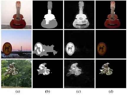
Fig. 1: Examples of our salient region detection from a trimap. (a) Inputs. (b) Trimaps. (c) Saliency maps. (d)
Salient regions.
The development of salient region detection has often been inspired by the concepts of human visual perception. One important concept is how ―distinct to a certain extent‖ [37] the salient region is compared to the other parts of an image. As color is a very important visual cue to human, many salient region detection techniques are built upon distinctive color detection from an image. In this paper, we propose a novel approach to automatically detect salient regions in an image. Our approach first estimates the approximate locations of salient regions by using a tree-based classifier. The tree-tree-based classifier classifies each super pixel as either foreground, background or unknown. The foreground and background are regions where the classifier classifies salient and non-salient regions with high confidence. The unknown regions are the regions with ambiguous features where the classifier classifies the regions with low confidence.
method and local learningbased method to estimate the saliency map. The results of these two methods will be combined together to form our final saliency map. Fig. 1 shows examples of our saliency map and salient regions from trimaps. The overview of our method is presented in
Fig. 2. Our algorithm is performed in superpixellevel in order to reduce computations (Fig. 2 (b)). The initial saliency trimap composed of a foreground candidate, background candidate, and unknown regions using existing saliency detection techniques are shown in Fig. 2 (c).
Fig. 2: Overview of our algorithm: (a) Input image. (b) Over-segmentation to superpixels. (c) Initial saliency trimap. (d) Global salient region detection via HDCT. (e) Local salient region detection via random forest. (f) Our final
saliency map.
The HDCT-based method is a global method. The motivation is to find color features which can efficiently separate salient regions and background, as illustrated in Fig. 4. The key idea is to exploit the power of different color space representations to resolve the ambiguities of colors in the unknown regions. The high dimensional color transform combines several representative color spaces such as red, green, and blue (RGB), CIELab, and HSV together with different power-law transformations to enrich the representative power of the HDCT space. Note that each of the color spaces has a different measurement about color similarity. For example, two colors in RGB with short distance may have long distance from each other in HSV or CIELab color spaces. Using the HDCT, we map a low-dimensional RGB color tuple into a high-low-dimensional feature vector. Starting from a few initial color examples of the detected salient regions and backgrounds, the HDCT-based method estimates an optimal linear combination of color values in the HDCT space that results in a per-pixel saliency map as shown in Fig. 2 (d).
The local learning-based method utilizes a random forest [50] with local features, i.e. relative location and color contrast between super pixels. Since the HDCT-based
method uses only color information, it can be easily affected by texture and noise. We overcome this limitation by using location and contrast features. If a super pixel is closer to the foreground regions than the background regions, it has higher chance to be a salient region. Based on this assumption, we train a random forest classifier to evaluate the saliency of a super pixel by comparing the distance and color contrast of a super pixel to the K-nearest foreground super pixels and the K-nearest background super pixels. Fig. 2 (e) shows an example of saliency map obtained by the local learning-based method. The value of K for the K-nearest neighbor is systemically found by measuring the performance of the local learning-based method on a validation set. We combine the saliency maps from the HDCT-based method and the local learning-based method by weighted combination (Fig. 2 (f)). Similar to the value of K in local learning-based method, the combination weights are determined by evaluating the performance of the saliency map on a validation set.
of saliency map. Although the work in [2] also utilizes spatial refinement to enhance performance of the HDCT-based method, our new local learning-HDCT-based method outperforms the spatial refinement method. The experimental results show that using the learning-based local saliency detection method, instead of the spatial refinement, significantly helps to improve the performance of our algorithm. Finally, we have also examined the effects of different initialization of trimap. We notice that by using the DRFI method [33] as the initial saliency trimap, we can further improve the performance of DRFI since our HDCT-based and local learning HDCT-based methods are able to resolve ambiguities in low confidence regions in saliency detection.
The key contributions of our paper are summarized as follows:
• An HDCT-based salient region detection algorithm [2] is introduced. The key idea is to estimate the linear combination of various color spaces that separate foreground and background regions.
• We propose a local learning-based saliency detection method that considers local spatial relations and color contrast between superpixels. This relatively simple method has low computational complexity and is an excellent complement to the HDCT-based global saliency map estimation method. In addition, the two resulting saliency maps are combined in a principled way via a supervised weighted sum-based fusion.
• We showed that our proposed method can further improve performance of other methods for salient region detection, by using their results as the initial saliency trimap.
The remainder of this paper is organized as follows. Section II reviews related works on salient region detection. Section III describes the initial trimap generation method. Section IV presents the two methods for saliency estimation from a trimap. It also introduces the HDCT-based global saliency estimation and regression-HDCT-based local saliency estimation methods. Section V presents the experimental results and comparisons with several state-of-the-art salient region detection methods. Section VI concludes our paper with discussions.
II. RELATED WORKS
This section reviews representative state-of-the-art salient region detection methods. A survey and a benchmark comparison of state-of-the-art salient region detection algorithms are presented in [3] and [4] respectively. As reported in [4], our HDCT-based method presented in [2] is one of the top six algorithms in salient region detection.
Local-contrast-based models detect salient regions by detecting rarity of image features in a small local region. Itti et al. [5] proposed a saliency detection method which utilizes visual filters called ―center-surround difference‖ to compute local color contrast. Harel et al. [6] suggested a graph-based visual saliency (GBVS) model which is based on the Markovian approach on an activation map. This model examines the dissimilarity of center-surround feature histograms. Goferman et al. [8] combined global and local contrast saliency to improve detection performance. Klein and Frintrop [10] utilized information theory and defined the saliency of an image using the Kullback-Leibler divergence (KLD). The KLD measures the center-surround difference to combine different image features to compute the saliency. Hou et al. [11] used the term ―information divergence‖ which expresses the non-uniform distribution of the visual information in an image for saliency detection.
Several methods estimated saliency in superpixel level instead of pixel-wise level to reduce the computational time. Jiang et al. [12] performed salient object segmentation with multiscale superpixel-based saliency and a closed boundary prior. Their approach iteratively updates both the saliency map and the shape prior under an energy minimization framework. Perazzi et al. [34] decomposed an image into compact and perceptually homogeneous elements, and then considered the uniqueness and spatial distribution of these elements in the CIELab color to detect salient regions. Yan et al. [14] used a hierarchical model by computing contrast features at different scales of an image and fused them into a single saliency map using a graphical model. Zhu et al. [42] proposed a background measure that characterizes the spatial layout of image regions with a novel optimization framework.
to give non-uniform weight to the same salient object when different features presented in the same salient object.
Global-contrast-based models use color contrast with respect to the entire image to detect salient regions. These models can detect salient regions of an image uniformly with low computational complexity. Achanta et al. [7] proposed a frequency-tuned approach to determine the center-surround contrast using the color and luminance in the frequency domain as features. Shen and Wu [35] divided an image into two parts—a low-rank matrix and sparse noise—where the former explains the background regions and the latter indicates the salient regions. Cheng et al. [40] proposed a Gaussian mixture model (GMM)-based abstract representation method that simultaneously evaluates the global contrast differences and spatial coherence to capture perceptually homogeneous elements and improve the salient region detection accuracy. Li et al. [43] showed that the unique refocusing capability of light fields can robustly handle challenging saliency detection problems such as similar foreground and background in a single image. He and Lau [46] used a pair of flash and no-flash images, inspired by the brightness of foreground objects for salient region detection.
These global-contrast-based models provide reliable results at low computational cost as they mainly consider a few specific colors that separate the foreground and the background of an image without using spatial relationships.
Statistical-learning-based models have also been examined for saliency detection. Wang et al. [15] proposed a method that jointly estimates the segmentation of objects learned by a trained classifier called the auto-context model to enhance an appearance-based energy minimization framework for salient region detection. Yang et al. [36] ranked the similarity of image regions with foreground cues and background cues using graph-based manifold ranking based on affinity matrices and successfully conducted saliency detection. Siva et al. [17] used an unsupervised approach to learn patches that are highly likely to be parts of salient objects from unlabeled images and then sampled the object saliency map to find object locations and detect saliency regions. Li et al. [39] proposed a saliency measure via dense and sparse representation errors of each image region using a set of background templates as the basis for reconstruction, and they constructed the saliency map by integrating multiscale reconstruction errors. Jiang et al. [41]
suggested a bottomup saliency detection algorithm that considers the appearance divergence and spatial distribution of salient objects and the background using the time property in an absorbing Markov chain. Lu et al. [45] used an optimal set of salient seeds obtained by learning a large margin formulation of the discriminant saliency principle.
As many novel saliency detection datasets have become available recently, supervised saliency estimation algorithms have also been proposed. Borji and Itti [16] used complementary local and global patch-based dictionary learning for rarity-based saliency in different color spaces—RGB and LAB—and then combined them into the final saliency map for saliency detection. Jiang et al. [33] proposed a multilevel image segmentation method based on the supervised learning approach that performed a regional saliency regressor using regional descriptors to build a saliency map to find salient regions.
These models are usually highly accurate and have a simple detection structure. However, they tend to require a lot of computational time. Therefore, superpixel-wise saliency detection is used to overcome the high computational complexity.
TABLE I
FEATURES USED TO COMPUTE FEATURE VECTOR FOR EACH SUPERPIXEL
III. INITIAL SALIENCY TRIMAP GENERATION
image in superpixel level. The initial saliency trimap consists of foreground candidate, background candidate, and unknown regions. A similar approach has already been used in a previous method [33], which demonstrated superiority and efficiency in their results. However, their algorithms require considerable computational time because their features’ computational complexity is very large. In our work, we only use some of the most effective features that can be calculated rapidly, such as color contrast and location features. As our goal in this step is to ―approximately‖ find the salient regions of an image, we found that the salient region could be found accurately using even a smaller number of features. By allowing for the classification of some ambiguous regions as unknown, we can further improve the accuracy of our initial saliency trimap.
A. Super pixel Saliency Features
As demonstrated in recent studies [33]–[36], features from superpixels are effective and efficient for salient object detection. For an input image I, we first perform over-segmentation to form superpixels X = {X1,..., XN }. We use the SLIC superpixel [1] because of its low computational cost and high performance, and we set the number of superpixels to N = 500. To build feature vectors for saliency detection, we combine multiple information that are commonly used in saliency detection. We first concatenate the superpixels’ x- and y-locations into our feature vector. The location feature is used because humans tend to focus more on objects that are located around the center of an image [18]. Then, we concatenate the color features, as this is one of the most important cues in the human visual system and certain colors tend to draw more attention than others [35]. We compute the average pixel color and represent the color features using different color space representations. Next, we concatenate histogram features as this is one of the most effective measurements for the saliency feature, as demonstrated in [33]. The histogram features of the ith superpixel DHi is measured using the chi-square distance between other superpixels’ histograms. It is defined as
where b is the number of histogram bins. In our work, we used eight bins for each histogram. We have also used the global contrast and local contrast as color features [7], [19], [34]. The global contrast of the ith superpixel DGi is given by
where d(ci, c j) denotes the Euclidean distance between the ith and the jth superpixels’ color values, c
i and cj, respectively. We use the RGB, CIELab, hue, and saturation of eight color channels to calculate the color contrast feature so that it has eight dimensions. The local contrast of the color features DLi is defined as
overall outline of the original image, and other smaller singular values depict detailed information. Therefore, some of the largest singular values occupy much higher weights for blurred images.
The aforementioned features are concatenated and are used to generate our initial saliency trimap. Table I summarizes the features that we have used. In short, our superpixel feature vectors consist of 71 dimensions that combine multiple evaluation metrics for saliency detection.
B. Initial Saliency Trimap via Random Forest Classification
After we calculate the feature vectors for every superpixel, we use a classification algorithm to check whether each region is salient. In this study, we use the random forest [50] classification because of its efficiency on large databases and its generalization ability. A random forest is an ensemble method that operates by constructing multiple decision trees at training time and decides the class by examining each tree’s leaf response value at test time. This method combines the bootstrap aggregating idea and random feature selection to minimize the generalization error. To train each tree, we sample the data with the replacement and train a decision tree with only a few features that are randomly selected. Typically, a few hundred to several thousand trees are used, as increasing the number of trees tends to decrease the variance of the model.
TABLE II
COMPARISON OF TRIMAP PERFORMANCE ON MSRA-B DATASET [49]
In our previous work [2], we used a regression method to estimate the saliency degree for each superpixel and classified it via adaptive thresholding. As our goal is to classify each superpixel as foreground and background, we found that using a classification method is more suitable than the regression for trimap generation. Table II shows a comparison of the trimap performance, in which the Fg. Precision (FP), Bg. Precision (BP), error rate (E R) are defined as below:
in which | · | denotes the number of pixels, FC and BC denote the foreground/background candidates, FGT and BGT denote the ground-truth annotations’ foreground/background, respectively, and I denotes the whole image. The error rate (E R) denotes the ratio of the area of misclassified regions to the image size, and the unknown rate is the ratio of the area of the regions classified as unknown to the image size. We used 2,500 images from the MSRA-B dataset [49], which are selected as a training set from Jiang et al. [33] for training data, and we used the annotated ground truth images for labels. We generated N feature vectors for each image. In total, we have approximately one million vectors for the training data.
Fig. 3: Some results of the initial saliency trimap. (a) Input image. (b) Binary map without unknown region.
(c) Our initial saliency trimap with unknown region indicated in gray color. (d) Ground truth.
IV. SALIENCY ESTIMATION FROM TRIMAP
In this section, we present our global salient region detection via HDCT and learning-based local salient region detection, and we describe a step-by-step process to obtain our final saliency map starting with the initial saliency map. In section IV-A, we propose a global saliency estimation method via HDCT [2]. The idea of global saliency estimation implicitly assumes that pixels in the salient region have independent and identical color distribution. With this assumption, we depict the saliency map of a test image as a linear combination of high-dimensional color channels that distinctively separate salient regions and backgrounds. In section IV-B, we propose a local saliency estimation via learning-based regression. Local features such as color contrast can reduce the gap between an independent and identical color distribution model implied by HDCT and true distributions of realistic images. In section IV-C, we analyze how to combine these two maps to obtain the best result.
A. Global Saliency Estimation via HDCT
Colors are important cues in the human visual system. Many previous studies [52] have noted that the RGB color space does not fully correspond to the space in which the human brain processes colors. It is also inconvenient to process colors in the RGB space as illumination and colors are nested here. Therefore, many different color spaces have been introduced, including YUV, YIQ, CIELab, and HSV. Nevertheless, which color space is the best for processing images remains unknown,
especially for applications such as saliency detection, which are strongly correlated to human perception. Instead of picking a particular color space for processing, we introduce a HDCT that unifies the strength of many different color representations. Our goal is to find a linear combination of color coefficients in the HDCT space such that the colors of salient regions and those of backgrounds can be distinctively separated. Fig. 4 illustrates the idea of using the linear combination of color coefficients for saliency detection.
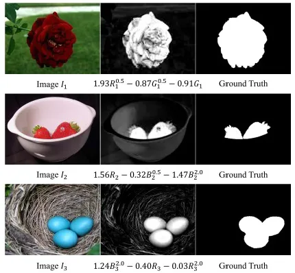
Fig. 4: Illustrations of linear coefficient combinations for HDCT-based saliency map construction. The first column images are input original images, the second column images are saliency maps which are obtained by
using a linear combination of RGB channels, and the third column images are ground truth saliency maps.
Fig. 5: Our HDCT space. We concatenate different nonlinear RGB transformed color space representations
to form a high-dimensional feature vector to represent the color of a pixel.
The different magnitudes in the color gradients can also be used to handle cases in which salient regions and backgrounds have different amounts of defocus and different color contrasts. In summary, 11 different color channel representations are used in our HDCT space. To further enrich the representative power of our HDCT space, we apply power-law transformations to each color coefficient after normalizing the coefficient between [0, 1]. We used three gamma values: {0.5, 1.0, and 2.0}.1 This resulted in a high-dimensional matrix to represent the colors of an image:
In which Ri and Gi denote the test image’s i th superpixel’s mean pixel value of the R color channel and G color channel, respectively. By using 11 color channels such as RGB, CIELab, hue, and saturation, we can obtain an HDCT matrix K with l = 11 × 3 = 33. The nonlinear power-law transformation takes into account the fact that our human perception responds nonlinearly to incoming illumination. It also stretches/compresses the intensity contrast within different ranges of color coefficients. Table III summarizes the color coefficients concatenated in our HDCT space. This process is applied to each superpixel in an input image individually.
TABLE III
SUMMARY OF COLOR COEFFICIENTS CONCATENATED IN OUR HDCT SPACE
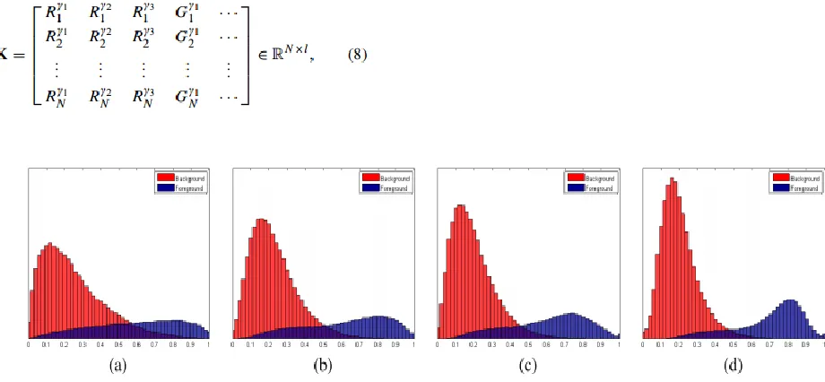
transformations; (c) RGB, CIELab, hue, and saturation; and (d) RGB, CIELab, hue, and saturation with power-law transformations. The overlap rate is (a) 16.49%, (b) 11.52%, (c) 9.92%, and (d) 5.84%.
To evaluate the effectiveness of the multiple color channels and power-law transformations, we use the LDA projection [24] on the 2,500 training images in the MSRA-B dataset [49] as used by Jiang et al. [33] to calculate the projection matrix and use the 500 validation set images for visualization. A self-comparison of our HDCT via LDA with other combinations of color channels is shown in Fig. 6. The result shows that the performance is undesirable when only RGB is used and that using various nonlinear RGB transformed color spaces and power-law transformations helps to classify the salient regions more accurately.
To obtain our saliency map, we utilize the foreground candidate and background candidate color samples in our trimap to estimate an optimal linear combination of color coefficients to separate the salient region color and background color. We formulate this problem as a l2 regularized least squares problem that minimizes
where α ∈ Rl is the coefficient vector that we want to estimate, λ is a weighting parameter to control the magnitude of α, and K is a M×l matrix with each row of K corresponding to color samples in the foreground/background candidate regions:
where FSi and BS j denote the i th foreground candidate superpixel among entire superpixels and the j th background superpixel among entire superpixels that are classified at the trimap generation step, respectively. M is the number of color samples in the foreground/background
candidate regions (M N), and f and b denote the number of foreground and background regions, respectively, such that M = f + b. U is an M dimensional vector with value equal to 1 and 0 if a color sample belongs to the foreground and background candidate, respectively:
Since we have a greater number of color samples than the dimensions of the coefficient vector, the l2 regularized least squares problem is a well-conditioned problem that can be readily minimized with respect to α as α∗ = (KT K + λI)−1KT U. In all experiments, we use λ = 0.05 to produce the best results. After we obtain α∗, the saliency map can be constructed as
B. Local Saliency Estimation via Regression
Although the HDCT-based salient region detection provides a competitive result with a low false positive rate, this method has a limitation in that it is easily affected by the texture of the salient region, and therefore, it has a relatively high false negative rate. To overcome this limitation, we present a learning-based local salient region detection that is based on the spatial and color distance from neighboring superpixels. Table IV summarizes the features used in this section. First, for each superpixel, we find the K -nearest foreground superpixels and K -nearest background superpixels as described in Fig. 7.
Fig. 7: An illustration of local saliency features. Black, white, and gray regions denote background superpixels,
foreground superpixels, and unknown superpixels, respectively. We use K -nearest foreground superpixels
and K -nearest background superpixels to calculate a feature vector.
For each superpixel Xi, we find the K -nearest foreground superpixels XFS = {XFS1, XFS2, . . . , XFSK } and K -nearest background superpixels XBS = {XBS1, XBS2, . . . , XBSK }, and we use the Euclidean distance between a
superpixel Xi and superpixels XF S or XBS as features. The Euclidean distance to the K-nearest foreground (dFSi ∈ RK×1) and background (d
BSi ∈ RK×1) features of the i th superpixel is defined as follows:
in which FSij denotes the jth nearest foreground superpixel and BSij denotes the jth nearest background superpixel from the i th superpixel. As objects tend to be located in a compact region in an image, the spatial distances between a candidate superpixel and the nearby foreground/background superpixels can be a very useful feature for estimating the saliency degree. We also use the color distance features between superpixels. The feature vector of color distances from the i th superpixel to the K-nearest foreground (dCFi∈ R8K×1) and background (d
CBi∈ R8K×1) superpixels is defined as follows:
TABLE IV
LOCAL SALIENCY FEATURES THAT ARE USED TO COMPUTE THE FEATURE VECTOR FOR EACH
SUPERPIXEL
are eight-dimensional color vectors. The distance vector d(ci, cF Sij ) is also an eight-dimensional vector, where each element of d(ci, cF Sij ) is the distance in a single color channel. To decide the optimal number of nearest superpixels K , we calculate the F-measure rate for each parameter. Fig. 8 shows the result, and we set K = 25, which shows the best result.2 For saliency estimation, we used the superpixel-wise random forest [50] regression algorithm, which is effective for large high-dimensional data.
Fig. 8: F-measure rate of validation results on different number of nearest superpixels K as features in the
MSRA-B dataset.
Fig. 9: Comparison of precision-recall curves of each step on the MSRA-B dataset.
We extracted feature vectors using the initial trimap, and then, we estimated the saliency degree for all superpixels. For this local saliency map, even those classified as foreground/background candidate superpixels
in the initial trimap are reevaluated because they could still be misclassified. It should be noted that the initial trimap is generated by a random forest classifier and that the next random forest regressor generates a local saliency map. Considering that we have two stages of cascaded random forests, we divided the training data set into two disjoint sets so that the second random forest is trained with more realistic inputs. Toward this end, we trained the first random forest with one data set, and we obtained the training data set for the second random forest from the trimaps generated for the other data set, which is not used for training the first random forest. This process is repeated in a manner similar to five-fold cross-validation. We used the code provided by Becker et al. [51] for random forest regression using 200 trees and setting the maximum tree depth to 10.
C. Final Saliency Map Generation
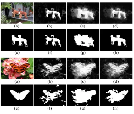
After we generated the global and the local saliency maps, we combined them to generate our final saliency map. Fig. 10 shows some examples of the two maps. Table V shows the quantitative performance measure of the two maps. The examples show that the HDCT-based saliency map tends to catch the object precisely; however, the false negative rate is relatively high owing to textures or noise. In contrast, the learning-based saliency map is less affected by noise, and therefore, it has a low false negative rate but a high false positive rate. Therefore, combining the two maps is a significant step in our algorithm.
TABLE V
QUANTITATIVE RESULTS OF HDCT-BASED GLOBAL SALIENCY DETECTION AND REGRESSION-BASED LOCAL SALIENCY ESTIMATION ON ADAPTIVE THRESHOLDED
Fig. 10: Some visual examples. (a) input image, (b) HDCT result, (c) local saliency estimation result, (d) combined result, (e) ground truth, (f)–(g) are adaptive
thresholded maps of (b)–(d), respectively
Borji et al. [38] proposed two approaches to combine the two saliency maps. The first approach is to perform the pixelwise multiplication of the two maps, as shown below:
In which Z is a normalization factor, p(.) is a pixel-wise combination function, SG is the global saliency result (Section IV-A), and SL is the local saliency result (Section IV-B). However, this combination tends to showdarker pixels and suppresses bright pixels, and therefore, some false negative pixels from a global saliency map will suppress the local saliency map, and the merit of the local saliency map will decrease. The second approach is to combine the two maps using a summation:
In our study, we combine the two maps more adaptively to maximize our performance. Based on Eq. (16), we adopt p(x) = exp(x) as a combination function to give greater weightage to the highly salient regions. The weight values are determined by comparing the saliency map with the ground truth. We calculate the optimal weight values for the linear summation by solving the nonlinear least-squares problem, as shown below:
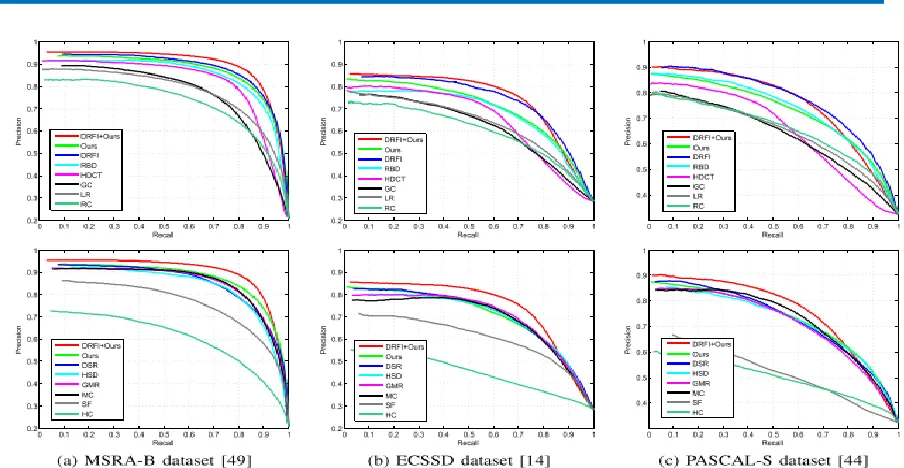
Fig. 11: Comparison of the precision-recall curve with state-of-the-art algorithms on three representative benchmark datasets: MSRA-B dataset, ECSSD dataset, and PASCAL-S dataset.
Fig. 10 (d) shows some examples of a combined map. We observe that the performance greatly improves after combining the two maps: highly salient regions that have been caught by the local saliency map are preserved, and the false negative region that is vaguely salient is discarded. To evaluate the effectiveness of our local saliency estimation, we compare the precision-recall curve with that of the spectral matting algorithm [48] that extracts foregrounds from the user input. We use the trimap result instead of the user input for automatic matting. Fig. 15 (h) shows some results. Although the matting algorithm can provide a reasonable result without being influenced by textures, we found that the matting method heavily relies on the input trimap and is therefore easily affected by misclassified superpixels. On the other hand, the learning-based method can determine the saliency degree by observing the spatial distribution of the nearest foreground and background superpixels, and therefore, our method is more robust to misclassified errors. Fig. 9 shows that the learning-based method provides a better result than the matting algorithm.
V. EXPERIMENTS
We evaluate and compare the performances of our algorithm against previous algorithms, including those
proposed by Zhai and Shah (LC) [9], Cheng et al. (HC, RC) [19], Shen and Wu (LR) [35], Perazzi et al. (SF) [34], Yan et al. (HS) [14], Yang et al. (GMR) [36], Jiang et al. (DRFI) [33], Li et al. (DSR) [39], Cheng et al. (GC) [40], Jiang et al. (MC) [41], and Zhu et al. (RBD) [42] as well as our own preliminary work (HDCT) [2] on three representative benchmark datasets: MSRA-B salient object dataset [49], Extended Complex Scene Saliency Dataset (ECCSD) [14], and PASCAL-S Dataset [44].
A. Benchmark Datasets for Salient Region Detection 1) MSRA-B Dataset: The MSRA-B salient object dataset [49] contains 5,000 images with the pixel-wise ground truth used by the authors provided by Jiang et al. [33]. This dataset mostly contains comparatively obvious salient objects in which the colors are definitely different from the background, and therefore, it is considered a less challenging dataset for salient object detection. We use the same training set including 2,500 images and the test set including 2,000 images used in [33] as the training and test data, respectively.
or a yellow butterfly on yellow flowers. In addition, many images contain a single salient object
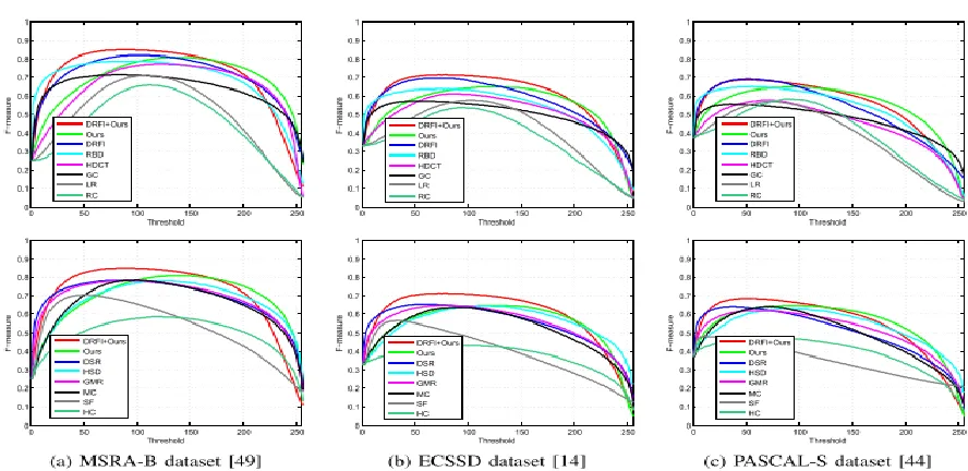
Fig. 12: Comparison of the F-measure curve with 12 state-of-the-art algorithms on three representative benchmark datasets: MSRA-B dataset, ECSSD dataset, and PASCAL-S dataset.
TABLE VI
COMPARISON OF THE PRECISION, RECALL, AND F-MEASURE RATE OF THE ADAPTIVELY THRESHOLDED SALIENCY MAP WITH STATE-OF-THE-ART ALGORITHMS ON THREE REPRESENTATIVE BENCHMARK DATASETS: MSRA-B DATASET, ECSSD DATASET, AND PASCAL-S DATASET. THE THREE BEST RESULTS
ARE HIGHLIGHTED IN RED, GREEN, AND BLUE, RESPECTIVELY
TABLE VII
COMPARISON OF AVERAGE RUN TIME (SECONDS PER IMAGE) OF THE MOST RECENT SALIENCY DETECTION ALGORITHMS
with multiple colors, making it harder to detect the salient object entirely. We used all images from this dataset for testing using the pixel-wise binary ground-truth images.
images with very large or very small salient objects that are relatively difficult to detect entirely. We used all images from this dataset for testing using the pixel-wise binary ground-truth images.
B. Performance Evaluation
In our study, we use two standard criteria for evaluating our salient region detection algorithm: precision-recall rate and F-measure rate. These evaluation criteria were proposed by Achanta et al. [7], and most saliency detection methods are evaluated by these criteria [3], [4].
Fig. 13: Some failure cases in PASCAL-S dataset [44]. (a) Original Image. (b) Ground Truth. (c) DRFI [33]. (d)
DRFI+ours.
1) Precision-Recall Evaluation: The precision is also called the positive predictive value, and it is defined as the ratio of the number of ground-truth pixels retrieved as a salient region to the total number of pixels retrieved as the salient region. The recall rate is also called the sensitivity, and it is defined as the ratio of the number of salient regions retrieved to the total number of ground-truth regions. We use two different approaches to examine the precision-recall rate. The first is to measure the rate for each pixel threshold. We bi-segment the saliency map using every threshold from 0 to 255 and calculate the precision rate and recall rate to plot the precisionrecall curve with the x-axis as the recall rate and the y-axis as the precision rate. The second is the precision and recall rate determined from the adaptively thresholded saliency map. In [7], [34], and [35], the threshold value is defined as two times the mean value of the saliency map. However, as recent saliency detection datasets, such as PASCAL-S [44], include some test images that contain a salient object that is larger than the background, we found that two times the mean value of the saliency map is not suitable for thresholding. Instead, we used the Otsu adaptive thresholding algorithm [47] to obtain the thresholded saliency map. We calculated the
precision and recall rate for every thresholded saliency map and evaluated it by averaging these values.
2) F-Measure Rate Evaluation: The second evaluation index is the F-measure rate. The F-measure combines the precision and the recall rate for a comprehensive evaluation. In our study, we used the Fβ measure, as defined below:
As in previous methods [7], [14], [35], we used β2 = 0.3. Similarly, as the precision-recall curve, we bi-segmented the map for every threshold and plotted the curve with the x-axis as the threshold and the y-axis as the F-measure rate. We also measured the F-measure rate from the adaptively thresholded saliency map. First, we drew the precision-recall (PR) curve and the F-measure curve of our entire algorithm, and to verify the effectiveness of saliency estimation after the trimap step, we used the final result obtained in Jiang et al. [33], which is a state-of-the-art method, as an initial map and used a simple thresholding method to transform it into a trimap. In Fig. 11, we indicate the PR curve of our entire algorithm as ―Ours‖ and that of the DRFI method-based trimap and our final saliency estimation algorithm as ―DRFI+Ours.‖ Similarly, in Fig. 12, we show the F-measure curve of the state-ofthe-art algorithms, including our method. Table VI shows the quantitative performance analysis of the adaptively thresholded saliency map. The results show that our methods achieved a competitive performance compared to the other methods, and when we substituted the DRFI [33] result map for the initial trimap, our method further improved the map and attained the best performance
Fig. 14. Some examples of failure cases. (a) Input images. (b) Our initial trimap. (c) Our results. (d)
Ground truth.
To further demonstrate the efficiency of our algorithm, we show the average computational time for each image of the state-of-the-art methods, including our algorithm. Table VII shows a comparison of the average run times of the three state-of-the-art methods. The running time is measured on a computer with an Intel Dual Core i5-2500K 3.30 GHz CPU. Considering that our method is implemented by using MATLAB with unoptimized code,
the computational complexity of the proposed method is comparable to that of other methods.
The experimental results show that our algorithm is effective and computationally efficient. Although our algorithm does not outperform DRFI [33], its computational speed is much higher. The result for the case in which we substitute the results of DRFI [33] for the initial trimaps indicates that if we obtain the trimap more accurately, we have more potential to obtain a better result. Fig. 15 shows some examples of salient object detection that demonstrate the effectiveness of our proposed method.
Fig. 15. Comparisons of our results and the results of previous methods. (a) Test image, (b) ground truth, (c) ours, (d) DRFI [33]+ours, (e) RBD [42], (f) DRFI [33], (g) HDCT [2], (h) matting [48], (i) GMR [36], (j) HS [14], (k) DSR [39],
(l) GC [40], (m) MC [41], (n) SF [34], (o) LR [35], (p) RC [19], and (q) HC [19].
In the PASCAL-S dataset, we found that the PR curve of DRFI+ours does not improve compared with DRFI. Fig. 13 shows some failure cases. As our method uses a fixed number of fore-/background superpixels K , our algorithm tends to highlight the most salient region with moderate size; therefore, our method is relatively weak against test images with very large or very small salient regions. In the case of the MSRA-B and ECSSD datasets, the DRFI+ours method shows the best performance
compared with the other state-ofthe-art methods, as they contain images with salient regions of moderate size.
C. Failure Cases
low-dimensional RGB space is very densewhere distributions of the foreground and background colors largely overlap, whereas in high-dimensional color space, the space is less dense and the overlap decreases, as shown in Fig. 6. Furthermore, if identical colors appear in both the foreground and the background or the initialization of the color seed estimation is very wrong, our result is undesirable. Fig. 14 shows some examples of failure cases. In the first row, the foreground and background have exactly the same color, and therefore, the initial trimap fails to classify the object as foreground. In the second row, the dog has the same color as the background, and therefore, our method only detects its tongue, which is of a different color compared to the background.
VI. CONCLUSION
We have presented a novel salient region detection method that estimates the foreground regions from a trimap using two different methods: global saliency estimation via HDCT and local saliency estimation via regression. The trimap-based robust estimation overcomes the limitations of inaccurate initial saliency classification. As a result, our method achieves good performance and is computationally efficient in comparison to the state-of-the art methods. We also showed that our proposed method can further improve DRFI [33], which is the best performing method for salient region detection. In the future, we aim to extend the features for the initial trimap to further improve our algorithm’s performance.
REFERENCES
[1] R. Achanta, A. Shaji, K. Smith, A. Lucchi, P. Fua, and S. Süsstrunk, ―SLIC superpixels compared to state-of-the-art superpixel methods,‖ IEEE Trans. Pattern Anal. Mach. Intell., vol. 34, no. 11, pp. 2274–2282, Nov. 2012.
[2] J. Kim, D. Han, Y.-W. Tai, and J. Kim, ―Salient region detection via high-dimensional color transform,‖ in Proc. IEEE Conf. Comput. Vis. Pattern Recognit. (CVPR), Jun. 2014, pp. 883–890.
[3] A. Borji, M.-M. Cheng, H. Jiang, and J. Li. (2014). ―Salient object detection: A survey.‖ [Online]. Available: http://arxiv.org/abs/1411.5878
[4] A. Borji, M.-M. Cheng, H. Jiang, and J. Li. (2015). ―Salient object detection: A benchmark.‖ [Online]. Available: http://arxiv.org/abs/1501.02741
[5] L. Itti, J. Braun, D. K. Lee, and C. Koch, ―Attentional modulation of human pattern discrimination psychophysics reproduced by a quantitative model,‖ in Proc. Conf. Adv. Neural Inf. Process. Syst. (NIPS), 1998, pp. 789–795.
[6] J. Harel, C. Koch, and P. Perona, ―Graph-based visual saliency,‖ in Proc. Conf. Adv. Neural Inf. Process. Syst. (NIPS), 2006, pp. 545–552.
[7] R. Achanta, S. Hemami, F. Estrada, and S. Susstrunk, ―Frequency-tuned salient region detection,‖ in Proc. IEEE Conf. Comput. Vis. Pattern Recognit. (CVPR), Jun. 2009, pp. 1597–1604.
[8] S. Goferman, L. Zelnik-Manor, and A. Tal, ―Context-aware saliency detection,‖ in Proc. IEEE Conf. Comput. Vis. Pattern Recognit. (CVPR), Jun. 2010, pp. 2376–2383.
[9] Y. Zhai and M. Shah, ―Visual attention detection in video sequences using spatiotemporal cues,‖ in Proc. ACM Multimedia, 2006, pp. 815–824.
[10] D. A. Klein and S. Frintrop, ―Center-surround divergence of feature statistics for salient object detection,‖ in Proc. IEEE Int. Conf. Comput. Vis. (ICCV), Nov. 2011, pp. 2214–2219.
[11] W. Hou, X. Gao, D. Tao, and X. Li, ―Visual saliency detection using information divergence,‖ Pattern Recognit., vol. 46, no. 10, pp. 2658–2669, Oct. 2013.
[12] H. Jiang, J. Wang, Z. Yuan, T. Liu, and N. Zheng, ―Automatic salient object segmentation based on context and shape prior,‖ in Proc. Brit. Mach. Vis. Conf. (BMVC), 2011, pp. 110.1–110.12.
[13] A. Y. Ng, M. I. Jordan, and Y. Weiss, ―On spectral clustering: Analysis and an algorithm,‖ in Proc. Conf. Adv. Neural Inf. Process. Syst. (NIPS), 2002, pp. 849–856.
[15] L. Wang, J. Xue, N. Zheng, and G. Hua, ―Automatic salient object extraction with contextual cue,‖ in Proc. IEEE Int. Conf. Comput. Vis. (ICCV), Nov. 2011, pp. 105–112.
[16] A. Borji and L. Itti, ―Exploiting local and global patch rarities for saliency detection,‖ in Proc. IEEE Conf. Comput. Vis. Pattern Recognit. (CVPR), Jun. 2012, pp. 478–485.
[17] P. Siva, C. Russell, T. Xiang, and L. Agapito, ―Looking beyond the image: Unsupervised learning for object saliency and detection,‖ in Proc. IEEE Conf. Comput. Vis. Pattern Recognit. (CVPR), Jun. 2013, pp. 3238–3245.
[18] T. Judd, K. Ehinger, F. Durand, and A. Torralba, ―Learning to predict where humans look,‖ in Proc. IEEE Int. Conf. Comput. Vis. (ICCV), Sep./Oct. 2009, pp. 2106– 2113.
[19] M.-M. Cheng, G.-X. Zhang, N. J. Mitra, X. Huang, and S.-M. Hu, ―Global contrast based salient region detection,‖ in Proc. IEEE Conf. Comput. Vis. Pattern Recognit. (CVPR), Jun. 2011, pp. 409–416.
[20] Z. Liu, R. Shi, L. Shen, Y. Xue, K. N. Ngan, and Z. Zhang, ―Unsupervised salient object segmentation based on kernel density estimation and two-phase graph cut,‖ IEEE Trans. Multimedia, vol. 14, no. 4, pp. 1275–1289, Aug. 2012.
[21] V. Navalpakkam and L. Itti, ―An integrated model of top-down and bottom-up attention for optimizing detection speed,‖ in Proc. IEEE Conf. Comput. Vis. Pattern Recognit. (CVPR), Jun. 2006, pp. 2049–2056.
[22] P. F. Felzenszwalb, R. B. Girshick, D. McAllester, and D. Ramanan, ―Object detection with discriminatively trained part-based models,‖ IEEE Trans. Pattern Anal. Mach. Intell., vol. 32, no. 9, pp. 1627–1645, Sep. 2010.
[23] B. Su, S. Lu, and C. L. Tan, ―Blurred image region detection and classification,‖ in Proc. ACM Int. Conf. Multimedia, 2011, pp. 1397–1400.
[24] R. O. Duda and P. E. Hart, Pattern Classification and Scene Analysis. New York, NY, USA: Wiley, 1973.
[25] H. Andrews and C. Patterson, ―Singular value decompositions and digital image processing,‖ IEEE Trans. Acoust., Speech, Signal Process., vol. 24, no. 1, pp. 26–53, Feb. 1976.
[26] Y.-S. Wang, C.-L. Tai, O. Sorkine, and T.-Y. Lee, ―Optimized scale-andstretch for image resizing,‖ ACM Trans. Graph., vol. 27, no. 5, p. 118, Dec. 2008.
[27] J. Park, J.-Y. Lee, Y.-W. Tai, and I. S. Kweon, ―Modeling photo composition and its application to photo re-arrangement,‖ in Proc. IEEE Int. Conf. Image Process. (ICIP), Sep./Oct. 2012, pp. 2741–2744.
[28] A. Ninassi, O. Le Meur, P. Le Callet, and D. Barbba, ―Does where you gaze on an image affect your perception of quality? Applying visual attention to image quality metric,‖ in Proc. IEEE Int. Conf. Image Process. (ICIP), vol. 2. Sep./Oct. 2007, pp. II-169–II-172.
[29] L. Marchesotti, C. Cifarelli, and G. Csurka, ―A framework for visual saliency detection with applications to image thumbnailing,‖ in Proc. IEEE Int. Conf. Comput. Vis. (ICCV), Sep./Oct. 2009, pp. 2232–2239.
[30] L. Itti, ―Automatic foveation for video compression using a neurobiological model of visual attention,‖ IEEE Trans. Image Process., vol. 13, no. 10, pp. 1304–1318, Oct. 2004.
[31] Y.-Y. Chuang, B. Curless, D. H. Salesin, and R. Szeliski, ―A Bayesian approach to digital matting,‖ in Proc. IEEE Conf. Comput. Vis. Pattern Recognit. (CVPR), vol. 2. Dec. 2001, pp. II-264–II-271.
[32] J. Wang and M. F. Cohen, ―Optimized color sampling for robust matting,‖ in Proc. IEEE Conf. Comput. Vis. Pattern Recognit. (CVPR), Jun. 2007, pp. 1–8.
[33] H. Jiang, J. Wang, Z. Yuan, Y. Wu, N. Zheng, and S. Li, ―Salient object detection: A discriminative regional feature integration approach,‖ in Proc. IEEE Conf. Comput. Vis. Pattern Recognit. (CVPR), Jun. 2013, pp. 2083–2090.
[35] X. Shen and Y. Wu, ―A unified approach to salient object detection via low rank matrix recovery,‖ in Proc. IEEE Conf. Comput. Vis. Pattern Recognit. (CVPR), Jun. 2012, pp. 853–860.
[36] C. Yang, L. Zhang, H. Lu, X. Ruan, and M.-H. Yang, ―Saliency detection via graph-based manifold ranking,‖ in Proc. IEEE Conf. Comput. Vis. Pattern Recognit. (CVPR), Jun. 2013, pp. 3166–3173.
[37] J. Feng, Y. Wei, L. Tao, C. Zhang, and J. Sun, ―Salient object detection by composition,‖ in Proc. IEEE Int. Conf. Comput. Vis. (ICCV), Nov. 2011, pp. 1028–1035.
[38] A. Borji, D. N. Sihite, and L. Itti, ―Salient object detection: A benchmark,‖ in Proc. IEEE Eur. Conf. Comput. Vis. (ECCV), Oct. 2012, pp. 414–429.
[39] X. Li, H. Lu, L. Zhang, X. Ruan, and M.-H. Yang, ―Saliency detection via dense and sparse reconstruction,‖ in Proc. IEEE Int. Conf. Comput. Vis. (ICCV), Dec. 2013, pp. 2976–2983.
[40] M.-M. Cheng, J. Warrell, W.-Y. Lin, S. Zheng, V. Vineet, and N. Crook, ―Efficient salient region detection with soft image abstraction,‖ in Proc. IEEE Int. Conf. Comput. Vis. (ICCV), Dec. 2013, pp. 1529–1536.
[41] B. Jiang, J. Zhang, H. Lu, C. Yang, and M.-H. Yang, ―Saliency detection via absorbing Markov Chain,‖ in Proc. IEEE Int. Conf. Comput. Vis. (ICCV), Dec. 2013, pp. 1665–1672.
[42] W. Zhu, S. Liang, Y. Wei, and J. Sun, ―Saliency optimization from robust background detection,‖ in Proc. IEEE Conf. Comput. Vis. Pattern Recognit. (CVPR), Jun. 2014, pp. 2814–2821.
[43] N. Li, J. Ye, Y. Ji, H. Ling, and J. Yu, ―Saliency detection on light field,‖ in Proc. IEEE Conf. Comput. Vis. Pattern Recognit. (CVPR), Jun. 2014, pp. 2806–2813.
[44] Y. Li, X. Hou, C. Koch, J. M. Rehg, and A. L. Yuille, ―The secrets of salient object segmentation,‖ in Proc. IEEE Conf. Comput. Vis. Pattern Recognit. (CVPR), Jun. 2014, pp. 280–287.
[45] S. Lu, V. Mahadevan, and N. Vasconcelos, ―Learning optimal seeds for diffusion-based salient object detection,‖
in Proc. IEEE Conf. Comput. Vis. Pattern Recognit. (CVPR), Jun. 2014, pp. 2790–2797.
[46] S. He and R. W. H. Lau, ―Saliency detection with flash and no-flash image pairs,‖ in Proc. IEEE Eur. Conf. Comput. Vis. (ECCV), Sep. 2014, pp. 110–124.
[47] N. Otsu, ―A threshold selection method from gray-level histograms,‖ IEEE Trans. Syst., Man, Cybern., vol. 9, no. 1, pp. 62–66, Jan. 1979.
[48] A. Levin, A. Rav Acha, and D. Lischinski, ―Spectral matting,‖ IEEE Trans. Pattern Anal. Mach. Intell., vol. 30, no. 10, pp. 1699–1712, Oct. 2008.
[49] T. Liu, J. Sun, N.-N. Zheng, X. Tang, and H.-Y. Shum, ―Learning to detect a salient object,‖ in Proc. IEEE Conf. Comput. Vis. Pattern Recognit. (CVPR), Jun. 2007, pp. 1– 8.
[50] L. Breiman, ―Random forests,‖ Mach. Learn., vol. 45, no. 1, pp. 5–32, Oct. 2001.
[51] C. Becker, R. Rigamonti, V. Lepetit, and P. Fua, ―Supervised feature learning for curvilinear structure segmentation,‖ in Proc. Int. Conf. Med. Image Comput. Comput. Assist. Intervent. (MICCAI), 2013, pp. 526–533.
[52] P. K. Kaiser and R. M. Boynton, Human Color Vision, 2nd ed. Washington, DC, USA: OSA, 1996.
Author Profile

![Fig. 13: Some failure cases in PASCAL-S dataset [44].](https://thumb-us.123doks.com/thumbv2/123dok_us/7752580.1271168/15.612.72.292.258.355/fig-some-failure-cases-in-pascal-s-dataset.webp)
