INVESTIGATION
A New Simple Method for Improving QTL
Mapping Under Selective Genotyping
Hsin-I Lee,* Hsiang-An Ho,* and Chen-Hung Kao*,†,1
*Institute of Statistical Science, Academia Sinica, Taipei 11529, Taiwan, Republic of China and†Division of Biometry, Institute of Agronomy, National Taiwan University, Taipei 10617, Taiwan, Republic of China
ABSTRACTThe selective genotyping approach, where only individuals from the high and low extremes of the trait distribution are selected for genotyping and the remaining individuals are not genotyped, has been known as a cost-saving strategy to reduce genotyping work and can still maintain nearly equivalent efficiency to complete genotyping in QTL mapping. We propose a novel and simple statistical method based on the normal mixture model for selective genotyping when both genotyped and ungenotyped
individuals arefitted in the model for QTL analysis. Compared to the existing methods, the main feature of our model is that wefirst
provide a simple way for obtaining the distribution of QTL genotypes for the ungenotyped individuals and then use it, rather than the
population distribution of QTL genotypes as in the existing methods, tofit the ungenotyped individuals in model construction. Another
feature is that the proposed method is developed on the basis of a multiple-QTL model and has a simple estimation procedure similar to that for complete genotyping. As a result, the proposed method has the ability to provide better QTL resolution, analyze QTL epistasis, and tackle multiple QTL problem under selective genotyping. In addition, a truncated normal mixture model based on a multiple-QTL model is developed when only the genotyped individuals are considered in the analysis, so that the two different types of models can be compared and investigated in selective genotyping. The issue in determining threshold values for selective genotyping in QTL mapping is also discussed. Simulation studies are performed to evaluate the proposed methods, compare the different models, and study the QTL mapping properties in selective genotyping. The results show that the proposed method can provide greater QTL detection power and facilitate QTL mapping for selective genotyping. Also, selective genotyping using larger genotyping proportions may provide roughly equivalent power to complete genotyping and that using smaller genotyping proportions
has difficulties doing so. The R code of our proposed method is available onhttp://www.stat.sinica.edu.tw/chkao/.
T
HE data in the QTL mapping study are usually composed of two parts, phenotypic trait values and marker geno-types, in the individuals, and the cost of producing data includes both phenotyping and genotyping costs. The cost ratio of the phenotyping to genotyping may vary signifi -cantly depending on the traits and species in studies. For afixed budget and time frame in the study, both costs must be considered and properly allocated to make the study optimally cost effective. If the total cost is not of primary concern in QTL experiments, all individuals in the entire sample will be genotyped and phenotyped for QTL analysis.However, QTL experiments are usually conducted under a limited budget, and researchers may not be allowed to genotype and phenotype a large amount of individuals for QTL analysis. It is hence necessary to make a reasonable and effective allocation for the genotyping and phenotyping costs in the experiment. The selective genotyping approach has been known as a cost-effective strategy for reducing genotyping work and still has the ability to maintain efficiency in QTL detection (Lebowitz et al. 1987; Lander and Botstein 1989). This approach is intended to select individuals with extreme (high and low) phenotypic values for genotyping and keep the remaining individuals ungenotyped in the entire sample. Later, several statistical methods have been proposed to study QTL mapping under selective genotyping (Darvasi and Soller 1992; Muranty and Goffinet 1997; Henshall and Goddard 1999; Xu and Vogl 2000; Manichaikul et al. 2007). They again
con-firmed that selective genotyping can achieve reasonable power and precision in detecting QTL as compared to complete Copyright © 2014 by the Genetics Society of America
doi: 10.1534/genetics.114.168385
Manuscript received July 15, 2014; accepted for publication September 16, 2014; published Early Online September 22, 2014.
1Corresponding author: Institute of Statistical Science, Academia Sinica, National Taiwan University, Taipei 115529, Taiwan, Republic of China.
genotyping but at the expense of moderate increase in the number of phenotyped individuals. As a larger number of individuals must be phenotypedfirst, before the required number of extreme individuals can be collected for genotyp-ing, selective genotyping will be most suitable for the cases in which the phenotyping cost is relatively inexpensive com-pared with the genotyping cost. Many economically and bi-ologically important traits, such asflowering time, fruit size and shape, crop (meat) yield or quality, growth in height and weight, plant stress and disease resistance, survival time, blood pressure, and body mass index in human, can be obtained at relatively low cost, and QTL mapping of these traits by using selective genotyping can be managed to be more cost effective than that by using complete genotyping. Consequently, although genotyping cost has been dropping recently, selective genotyping has been still widely em-ployed in QTL mapping for improving these traits and un-derstanding their genetic basis in several plant and animal species (Abdel-Haleem et al. 2011; Lu et al. 2013; Miller
et al. 2013; Fontanesi et al. 2014;). The keyword search using Google Scholar also reveals that selective genotyping remains popular and is more frequently used in genetics studies in recent years. The reasons may be that as marker genotyping becomes cheaper, more researchers are attracted to the QTL mapping analysis, but still face the situation of insufficient budgets to fully cover the expense of complete genotyping, and selective genotyping can become an alter-native, cost-effective choice that allows maintenance of sim-ilar efficiency to complete genotyping in QTL mapping.
In general, the statistical methods of QTL mapping for selective genotyping can be grouped into two major types according to whether their models take the ungenotyped individuals (ungenotyping data) into account in the analy-sis. Methods of the first type use only the genotyped individuals (genotyping data) and exclude the ungenotyp-ing data to develop statistical models for QTL analysis (Darvasi and Soller 1992; Henshall and Goddard 1999; Xu and Vogl 2000). Darvasi and Soller (1992) calculated the trait means of the QTL genotypes from the selected tails and constructed at-test for their difference to determine linkage between a marker and a QTL in the backcross population. Henshall and Goddard (1999) used a logistic regression ap-proach to the analysis of selective genotyping data by treat-ing phenotypes as independent variables and genotypes as dependent variables for QTL mapping. Xu and Vogl (2000) developed a truncated normal mixture model for the inter-val mapping procedure under the framework of selective genotyping in QTL detection. Methods of the second type consider both genotyped and ungenotyped individuals (full data) from selective genotyping for QTL analysis (Muranty and Goffinet 1997; Roninet al.1998; Xu and Vogl 2000). By analyzing full data, Muranty and Goffinet (1997) adopted a normal mixture model to detect QTL under selective genotyping in the backcross population. Roninet al. (1998) proposed a mixture model for the study of interval mapping of two QTL under selective genotyping. Xu and Vogl (2000)
also used a normal mixture model to tackle the issue of QTL mapping under selective genotyping in the F2population. In
their normal mixture models, the mixing proportions for different QTL genotypes of the genotyped individuals are determined by the flanking markers as usual, and those of the ungenotyped individuals are assigned by the population frequencies (e.g., 1/2 and 1/2 in the backcross, and 1/4, 1/2, and 1/4 in the F2population for a single-QTL model). When
comparing the two types of methods in selective genotyping, Xu and Vogl (2000) suggested that whenever possible, the analyses on full data are preferred over those on genotyping data, since the formers tend to provide improved estimations and greater test statistics for QTL parameters.
In this article, we develop a novel and simple statistical method on the basis of a normal mixture model to analyze full data from selective genotyping for QTL detection. Compared to the existing methods (Muranty and Goffinet 1997; Roninet al.1998; Xu and Vogl 2000), the main nov-elties of our proposed method are twofold. Thefirst novelty is that we obtain the proportions of QTL genotypes in the ungenotyped individuals by deducting the expected QTL frequencies in the genotyped individuals from their popula-tion frequencies. Then these proporpopula-tions instead of the pop-ulation QTL frequencies, as in the existing methods, are used to model the ungenotyped individuals in model con-struction, so that the proposed model can fit better to the data and yield better performance in selective genotyping. The second novelty is that our proposed model is developed on the basis of a multiple-QTL model, as has been done in QTL mapping for complete genotyping (Kao et al. 1999). The multiple-QTL model approach can take multiple QTL into account to control more genetic variation for improving QTL detection. As a result, with the novelties, our proposed method can provide better resolution, analyze epistasis, and tackle multiple QTL problems in QTL mapping under selec-tive genotyping. In addition, a truncated normal mixture model based on the multiple-QTL model is developed when only genotyping data are used in the analysis. We then com-pare the differences in QTL mapping between the two types of selective genotyping methods and investigate their prop-erties under the multiple-QTL framework, as their notable differences blurred in the single-QTL framework may appear in the multiple-QTL framework. The threshold values of selective genotyping for different models are also investi-gated. Simulation studies are conducted to evaluate the pro-posed method, compare different models, and study their properties in QTL mapping under selective genotyping.
The Statistical Methods for Selective Genotyping
individuals with marker genotypes and ungenotyping data containing intermediate individuals without marker genotypes. As described in the Introduction, statistical QTL mapping methods for analyzing selective genotyping data can either take full data or take just genotyping data into account in their models for QTL detection. When considering full data in the analysis, it is important to know that the genotypic frequencies of QTL in the ungenotyping (or genotyping) data are no longer the same as those in the full data, and they will depend on the underlying QTL parameters and population structures. With such facts, we obtain the frequencies of QTL genotypes in the ungenotyped individuals and use them, rather than the population frequencies of QTL genotypes as in the existing methods, to model the ungenotyped individuals and then to propose a new normal mixture model for QTL mapping when full data are used in the analysis. As opposed to our proposed method, the existing methods using normal mixture model will hereinafter be called population frequency-based (PFB) meth-ods. Furthermore, we also develop a truncated normal mixture model for QTL mapping when only genotyping data are used in the analysis. Both types of models are developed on the basis of a multiple-QTL approach, so that they can be compared under QTL analyses and be used to deal with the multiple-QTL problem. In the following, wefirst investigate the genotypic distributions in the genotyped and ungenotyped individuals, then present the truncated model, andfinally outline our proposed method for selective genotyping.
Genotypic distributions in the genotyped and ungenotyped individuals
In the F2 population, a QTL, Q, under consideration has
three possible genotypes, QQ, Qq, and qq with expected frequencies 1/4, 1/2, and 1/4, respectively. Their genotypic values, G2, G1, and G0, can be related to genotypic mean (m), additive effect (a), and dominance effect (d) by
G¼ 0 @GG21
G0
1 A¼
0 @11
1
1 Amþ
0 B B B B B B B @
1 21
2
0 1
2
21 21 2
1 C C C C C C C A
a d
¼13 mþDE;
(1)
where Dis known as the genetic design matrix for charac-terizing the genetic effects of QTL in the vector E. Under such settings, the trait value of an individual,yi, affected by
Qmay have three possible distributions,i.e.,yi|QQN(m1,
s2),y
i|QqN(m2,s2), oryi|qqN(m3,s2), wherem1,m2, andm3are the corresponding genotypic values. If a selective genotyping approach with genotyping proportion u (u/2 from each tail) is conducted on a sample with sizeN,N3 u individuals from the two tails will have both trait and marker information, andN3(12u) individuals from the middle will have only trait information. LetTRandTLbe the right and left truncated points so thatP(yi,TL) =P(yi.
TR) =u/2. ForNlarge enough, the expected genotypic fre-quencies in the ungenotyped individuals arewj3[F((TR2
mj)/s)2F((TL2mj)/s)],j= 1, 2, 3, whereF() denotes a standard normal cumulative distribution function, andw1= 1/4, w2 = 1/2, and w3 = 1/4 are the expected genotypic frequencies in the whole population. Then, the proportions of the three QTL genotypes in the ungenoytyped individuals can be straightforwardly obtained by
kj¼ wj
Ft2j
2Ft1j P3
k¼1wk½Fðt2kÞ2Fðt1kÞ
; j¼1;2;3; (2)
where t1j¼ ðTL2mjÞ=s and t2j¼ ðTR2mjÞ=s. As kj’s are functions of truncated points (TLand TR), genetic parame-ters (m,a,d, ands), and population frequencies (wj’s), the values ofkj’s depend on the factors such as genotyping pro-portions, heritability, sizes and modes of QTL actions, and population structure. For example, ifa =d= 1,h2= 0.5,
and u = 0.5 (P(yi , TL) = P(yi . TR) = 0.25), the two truncated points are TL ffi 20.785 and TR ffi 0.873. The genotypic frequencies of QQ, Qq, and qq are about 0.017 (0.083), 0.034 (0.166), and 0.199 (0.001) among the genotyped individuals in the left (right) extreme, about 0.150, 0.299, and 0.051 among the ungenotyped individuals, respectively. Then, k1 = 0.299 (ffi0.150/0.5), k2 = 0.599 (ffi0.299/0.5), and k3 = 0.101 (ffi0.051/0.5), respectively, by Equation 2. Similarly, these genotypic proportions are 0.069 (0.332), 0.137 (0.665) , and 0.794 (0.003) for yi,
TL (yi.TR), respectively. Essentially, it is worth noting that the expected proportions of the three QTL genotypes in the genotyped and ungenotyped samples are no longer wj’s like those in the whole sample.
Equation 2 can be easily extended to the multiple-QTL case for obtaining the genotypic proportions in the ungenotyped population. For example, in the case of two QTL, Q1 and
Q2, there are nine possible QTL genotypes, Q1Q1Q2Q2,
Q1Q1Q2q2, Q1Q1q2q2, Q1q1Q2Q2, Q1q1Q2q2, Q1q1q2q2,
q1q1Q2Q2, q1q1Q2q2, q1q1q2q2, respectively. Their expected population frequencies arew1= (12r)2/4,w2=r(12r)/
2,w3=r2/4,w4=r(12r)/2,w5= (12r)2/2 +r2/2,w6= r(12r)/2,w7=r2/4, w8=r(12r)/2,w9= (12r)2/4,
respectively, whereris the recombination fraction between the two QTL. For r = 0.3, the values ofwj’s are 0.123, 0.105, 0.023, 0.105, 0.290, 0.105, 0.023, 0.105, and 0.123, respectively. If the two QTL have effects (a1= 3, d1= 1,
a2= 1,iaa= 2) andh2= 0.5, the values ofk
values ofwj’s andkj’s. Our proposed QTL mapping method for selective genotyping intends to use kj’s rather than wj’s to model the relationship between the trait values and unobserv-able genotypes in the ungenotyped individuals.
The genetic model for multiple QTL, saymQTL, can be easily obtained from Equation 1 by augmenting the dimen-sions of the genetic design matrix according to their effects under consideration. Then, on the basis of the genetic model, the statistical model for fitting these m QTL, Q1,
Q2,. . .,Qm, without epistasis at given positions within the
m separate marker intervals, (M1,N1), (M2,N2), . . ., (Mm,
Nm), can be written as
yi¼mþX m
k¼1
akxik* þdkz*ik þei;i¼1;2;⋯;n; (3)
wherex*
ik’s andz
*
ik’s are coded variables for the additive and dominance effects,ak’s anddk’s, for Qk’s,k= 1, 2,. . .,m,yi is the quantitative trait value of theith individual, andeiis a random error and assumed to followN(0,s2). Note that x*
ikandz
*
ikassociated withakanddkare coded as (1,21/2), (0, 1/2), and (21, 21/2) for genotypes QkQk, Qkqk, and
qkqk, respectively, and the above model can be easily ex-tended to the model with epistasis by introducing the product terms as the terms for epistasis. Under complete genotyping, the likelihood function of the statistical model for the param-etersQis a mixture of 3mnormals as
LðQjY;XÞ ¼Y n
i¼1
X3m
j¼1
pijf
yijmj;s2 ; (4)
wheref(yi|mj,s2) is a normal p.d.f. with meanmjand var-iance s2,m
j’s correspond to the genotypic values of the 3m QTL genotypes, andpij’s are the mixing proportions inferred from theirflanking marker genotypes. If the statistical model is applied to analyze the data from selective genotyping, the likelihood will be different and depend on whether all indi-viduals or just genotyping indiindi-viduals are considered in the model as described below.
Model to analyze only genotyping data
Under selective genotyping, suppose that, among then indi-viduals, nsindividuals with extreme trait values (ns/2 each from the upper and lower extremes) are selected for marker genotyping, and the remainingnu(nu=n2ns) individuals are not genotyped. If only the genotyped individuals from the two extremes are utilized in the analysis, data of this sort are called centrally truncated data and the methods of ana-lyzing truncated data can be applied to the analyses (Cohen 1991). Xu and Vogl (2000) incorporated the truncated model into the mixture structure of interval mapping frame-work to propose a truncated normal mixture model for QTL analysis. They pointed out that the maximization of the truncated normal mixture likelihood is a challenging task, and they used an EM algorithm to obtain the maximum likelihood estimates (MLE) of the QTL parameters for the
model. An investigation of detection of a single QTL under selective genotyping was performed in their analysis. Here, we provide an alternative version of the EM algorithm for obtaining the MLE of the truncated normal mixture model and use it to address more complicated issues involving mapping multiple QTL and analyzing their epistasis. Forns
genotyped individuals, the likelihood function forQis
LðQjY;XÞ ¼Y ns
i¼1
X3m
j¼1
pij f
yijmj;s2
Uj ;
(5)
where pij’s are the conditional probabilities of QTL geno-types given marker genogeno-types, f(yi|mj, s2) is the normal density with meanmjand variances2, and
Uj¼ Z TL
2Nf
yijmj;s2 dyiþ Z N
TR f
yijmj;s2 dyi
¼Ft1j
þ12Ft2j
is the cumulative density with genotypic values greater thanTRand lower thanTL. Statistically, the normal density
f(yi|mj,s2) is standardized byUjto become a truncated nor-mal densityf(yi|mj,s2)/Uj. The details of the EM algorithm for obtaining the MLE of the parameters in the truncated normal mixture likelihood are described inAppendix. In sum-mary, the (t+ 1)th iteration of the EM step is given below.
E-step: Update the posterior probabilities of the 3m QTL genotypes,
pij¼ pijf
yijmj;s2
. Uj P3m
k¼1pikfðyijmk;s2Þ=Uk
forj= 1, 2,. . ., 3m,i= 1, 2,. . .,n s.
M-step: Find the estimates to maximize the conditional log-likelihood (seeAppendix). Equivalently, we can obtain the estimates from the following equations. For m, the QTL effects, ands2, the equations are
mðtþ1Þ¼ 1 ns
h
19nsY2PðtÞDEðtþ1Þ þRðtÞmi; (6)
Eðtþ1Þ¼rðtÞ2MðtÞEðtÞþRðtÞ
E ; (7)
s2ðtþ1Þ¼ 1 ns2RðtÞs2
Y2mðtþ1Þ1ns 9
Y2mðtþ1Þ1ns
22
Y2mðtþ1Þ1ns 9PðtÞDEðtþ1Þ
þEðtþ1Þ9VðtÞEðtþ1Þo;
(8)
whereP¼ fpijgns33mcontains the posterior probabilities of
QTL genotypes for the ns genotyped individuals, E is a
effects (e.g.,E231= [a d]9for a single-QTL model
con-sidering the additive and dominance effects),
r¼ ðY2m1nsÞ9P Di 19n
sPðDi#DiÞ k31
; M¼ 19nsP
Di#Dj
19n
sPðDi#DiÞ
3dði6¼jÞ
( )
k3k ;
) (
Rm¼
h
19n
sPA
i
s; RE¼ A
(
19n
sPðDi#AÞs
19nsPðDi#DiÞ A
)
k31
; Rs2¼19n
sPB;
and V¼ f19nsPðDi#DjÞgk3k. In the above expressions, Rm,
RE, and Rs2 are the correction terms to mainly account
for the truncated normal distributions,Diis ak31 col-umn vector in the genetic model that associate with the corresponding QTL effect in theith element ofE, anddis an indicator variable. Also,
A¼
( ft1j
2ft2j
Ft1j
þ12Ft2j
)
3m31
and
B¼
( t1jf
t1j
2t2jf
t2j
Ft1j
þ12Ft2j
)
3m31
;
where f() denotes the normal density function from the derivatives of logUj(seeAppendix) and are key components in Rm, RE, andRs2. The E and M steps are iterated until
convergence. The converged values ofm,E, ands2are the
MLEs. We intended to express the solutions of the parame-ters (Equations 6–8) in the general formulas format designed for complete genotyping (Kao and Zeng 1997), so that the two sets of equations can be compared and investigated un-der complete and selective genotyping. When all individuals are genotyped for markers and included in the analysis, the correction terms in Equations 6–8 vanish, and the equations reduce to the same equations for complete genotyping.
Model to analyze full data
If all thenindividuals, including thensgenotyping individ-uals and nu ungenotyping individuals, are fitted into the statistical model (Equation 3) for QTL analysis, the model likelihood can be written as
LðQjY;XÞ ¼Y ns
i¼1
X3m
j¼1
pijf
yijmj;s2 3Y nu
i¼1
X3m
j¼1
qjf
yijmj;s2 ;
(9)
where thefirst and second terms on the right-hand side are the likelihoods for thensgenotyped and for thenu ungen-otyped individuals, respectively. Both likelihoods are normal mixture densities as the QTL genotypes are not observed. In the likelihood for the ns genotyped individuals, the mixing proportions, pij’s, of a genotyped individual iare obtained
from the conditional probabilities of the QTL genotypes given itsflanking marker genotype. In the likelihood for the
nuungenotyped individuals, each different individual mixture density will be given to the same mixing proportions qj’s. Since there is no marker available to infer qj’s, ideally, we would use kj’s (Equation 2),i.e., the proportions of QTL genotypes in the ungenotyped individuals (seeGenotypic dis-tributions in the genotyped and ungenotyped individuals), to serve as the role of qj’s in the likelihood from the ungeno-typed individuals. However, the values of kj’s depend on the unknown QTL parameters, which will complicate the maximum-likelihood estimation if used directly. To avoid the complication, the PFB methods usewj’s asqj’s in their models,
e.g.,q1=w1= 1/4,q2=w2= 1/2, andq3=w3= 1/4 form= 1 in the F2model. Here, we propose the quantities
aj¼P3mwj2bj k¼1ðwk2bkÞ
; j¼1;2;⋯;3m; (10)
for the approximation ofkj’s and useaj’s asqj’s in our pro-posed method. Inaj,bjis given as
bj¼ Pns
i¼1pij
n ;
which sums up the conditional probabilities of a QTL genotype (indexed by j) over the ns genotyped individuals (indexed by i) and then divides the sum byn. Therefore, bj is the expected frequency of a QTL genotype among the ge-notyped individuals in the whole sample. By subtractingbjfrom its corresponding population frequencywj,i.e., (wj2bj), we can obtain the expected frequency of a QTL genotype among the ungenotyped individuals in the whole sample. The pro-posed quantities aj’s in Equation 10 reweigh these subtracted quantities, so that they are summed up to one and can serve as the proportions of QTL genotypes in the ungenotyped individuals for the use ofqj’s in Equation 9. Equation 10 can be better un-derstood by the following example: In the F2population (w1=
0.25,w2= 0.5, andw3= 0.25), if only one QTL coincident with a marker is considered, the expected genotypic frequen-cies are equivalent to the observed frequenfrequen-cies in the geno-typed individuals. Underu = 0.5, assume that the observed genotypic frequencies are 0.1, 0.2, and 0.2, respectively, in the genotyped individuals, thenb1= 0.1,b2= 0.2, andb3= 0.2. Consequently, we can havea1= 0.3,a2= 0.6, anda3= 0.1 by Equation 10. In practice, QTL are usually not coinci-dent with markers, and the expected genotypic frequencies
pij’s will be used in obtainingbj’s and thenaj’s. On very rare occasions, a negative value may occur inwj2bj, and a zero value is suggested as a replacement. Equivalently, we propose
aj¼
max
n
0;wj2bj o
P3m
k¼1maxf0;wk2bkg
; j¼1;2;⋯;3m; (11)
is as simple as the PFB methods in that the mixing propor-tions arefixed and need not be estimated, so that the esti-mation procedures are similar to those of the QTL mapping model under complete genotyping. In the parameter estima-tion, the EM algorithm for complete genotyping (Kao and Zeng 1997) can be directly applied to obtain the MLE for our proposed model. In E step, we update the posterior proba-bilities of QTL genotypes for the ns genotyped individuals andnuungenotyped individuals,
psij¼ pij f
yijmj;s2 P3m
k¼1pik fðyijmk;s2Þ
and puij ¼ qj f
yijmj;s2 P3m
k¼1qk fðyijmk;s2Þ
;
respectively, at the current estimates of the parameters. In M step, the solutions of the parameters,m,s2, and QTL effects
have the same formulations as Equations 6–8 except that the correction terms, Rm, RE, and Rs2, vanish. Certainly, the
posterior probability matrix must be adjusted to P¼ ½fpsijgns33m fpuijgnu33m9according to the numbers of
genotyped and ungenotyped individuals. The E and M steps are iterated until convergence. The converged values of esti-mates are the MLEs. Second, because aj’s are estimates of the proportions of QTL genotypes in the ungenotyped indi-viduals, our proposed model usingaj’s as mixing proportions willfit better to the ungenotyped individuals when compared to the PFB method using wj’s. As a result, the proposed method can be more powerful in QTL detection under selec-tive genotyping as is validated in the simulation study.
Simulation Result
Simulations were performed to evaluate the performance of our proposed method and to compare it with the currently used methods in QTL mapping under selective genotyping. Assume that a quantitative trait of interest is controlled by two unlinked epistatic QTL, QAand QB, in the F2population.
The two QTL are placed at 52 and 93 cM of two 150-cM chromosomes. Assume QAhas additive (a1) and dominance
effects (d1), and QB has only additive effect (a2). Epistasis
between QTL is assumed to be present only for the additive by additive effect (iaa). Further, assume four scenarios, (a1= 3,
d1= 1,a2= 1,iaa= 2), (a1= 2,d1= 1,a2= 1,iaa= 2), (a1= 1,d1= 1,a2= 1,iaa= 2), and (a1=21,d1= 1,a2= 1,iaa= 2), for the four present effects, which can reflect the relative sizes of the two QTL and epistasis. For (a1 = 3,
d1= 1,a2= 1,iaa= 2), QAand QBcontribute 76 and 8%
to the total genetic variance (VQ A=VG ¼ 76% and
VQ B=VG ¼ 8%), and epistasis contributes 16% to the total genetic variance (VI/VG= 16%). Similarly, (VQ A=VG ¼ 60%,
VQ B=VG ¼ 13:3%,VI=VG ¼ 26:7%) for (a1= 2,d1= 1,a2= 1, iaa = 2), (VQ A=VG ¼ 33:3%, VQ B=VG ¼ 22:2%, VI=VG ¼ 44:4%) for both (a1= 1,d1= 1,a2= 1,iaa= 2) and (a1=21,d1= 1,a2= 1,iaa= 2). For each scenario of the effect setting, two kinds of marker maps, 5 and 15 cM, two heritabilities of the quantitative trait, 0.1 and 0.2, and two
levels of selective genotyping proportions, 50 and 20%, are considered. The sample size is 200 for selective proportion 50% (the 100/200 design), and it is 500 for selective pro-portion 20% (the 100/500 design). Three models, the PFB model, the proposed model, and truncated model (Xu and Vogl 2000), are used for selective genotyping analysis. Also, the results of complete genotyping in the 100/100, 200/200, and 500/500 designs are presented for comparison. The number of simulated replicate is 1000. A stepwise selection procedure (Kaoet al.1999) was adopted to detect QTL and analyze epistasis. Threshold value of QTL mapping for selec-tive genotyping has been found to be similar to that for com-plete genotyping (Muranty and Goffinet 1997; Manichaikul
et al. 2007). We have further confirmed that the threshold values for selective genotyping are similar among the three different methods and among the two different designs based on 10,000 simulation replicates (results not shown). Here, the approximate threshold values for complete genotyping obtained by Gaussian stochastic process (Kao and Ho 2012) are used as those for selective genotyping. The obtained val-ues at 5% level are 9.18 (9.80) and 12.34 (13.35) for one and two degrees of freedom in the 15-cM (5-cM) marker map, respectively.
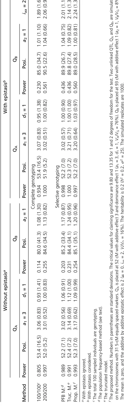
To shorten the article, the results for the scenario of (a1 = 3, d1 = 1, a2 = 1,iaa = 2) are reported in detail regarding the power and estimation (Table 1, Table 2, Table 3, and Table 4), and the results of the other scenarios are reported only for power (Table 5). For the (a1= 3,d1= 1,
a2= 1, iaa= 2) scenario, the analyses using the one-QTL model of the three selective genotyping methods are first applied to QTL detection. Under the one-QTL model, the three methods have similar performance in detection power and parameter estimation of QTL effects and positions (results not shown). The powers of the three methods to detect the larger QTL, QA, are all close to 100%. And their
powers to detect the smaller QTL, QB, in the 15- and 5-cM
marker maps are16% and18% under the 100/200 de-sign and are 24% and 27% under the 100/500 design. Further analyses using the multiple-QTL model are then followed for all the complete and selective genotyping meth-ods. Table 1 and Table 2 show the results of QTL mapping under complete genotyping (with the 100/100 and 200/200 designs) and selective genotyping (with the 100/200 de-sign) when epistasis is ignored and considered in the 5- and 15-cM marker maps. In general, for all methods and designs, greater power in detection and better quality in estimation can be achieved when the marker map is denser and epistasis is taken into account. The results for consider-ing epistasis in the analyses are described here. In the com-plete genotyping 100/100 design, the powers of detecting QAand QBare 93.4% (90.3%) and 23.0% (19.6%),
99.8% (99.4%) and 43.6% (38.5%), the powers by the trun-cated model are 100% (99.5%) and 43.6% (38.1%), and the powers by the proposed method are 99.7% (99.5%) and 56.0% (49.8%) in the 5-cM (15-cM) marker map, respec-tively. It shows that the proposed method is more powerful in QTL detection than the PFB method and truncated model and that the proposed method in the 100/200 design has the ability to provide similar power to complete genotyping under the two marker maps. All methods for selective genotyping methods provide similar precision and accuracy in the estimation of QTL positions. For example, in the 5-cM marker map, the means of the estimated QA and QB
posi-tions by the PFB method, truncated model, and proposed method are at 52.2 cM (SD 7.0 cM) and 89.9 cM (SD 26.7 cM), 52.3 cM (SD 7.2 cM) and 89.8 cM (SD 27.4 cM), and 52.2 cM (SD 7.0 cM) and 89.0 cM (SD 28.5 cM), respec-tively. In the estimation of the QTL effects, the three meth-ods generally perform well, as their means of the estimated effects are all very close to the true value. For example, in the 5-cM marker map, the means of the two estimated ad-ditive effects are 3.02 (SD 0.57) and 1.04 (SD 0.75) by the PFB method. The means are 3.21 (SD 0.71) and 1.09 (SD 0.82) by the truncated model, and the means are 3.20 (SD 0.64) and 1.00 (SD 0.81) by the proposed method. The epistatic effect between QTL can be also estimated well in selective genotyping. The means of estimated epistatic effects are 2.01 (SD 1.15), 2.14 (SD 1.35), and 2.24 (SD 1.36), respectively. In complete genotyping, their means are 1.89 (SD 1.68) and 2.06 (SD 0.98) for the 100/100 and 200/200 designs, respectively.
Table 3 and Table 4 show the results of QTL mapping under complete genotyping (with the 100/100 and 500/500 designs) and selective genotyping (with the 100/500 de-sign) when epistasis is ignored and considered in the 5- and 15-cM marker maps. Again, for all methods and designs, greater power in detection and better quality in estimation can be achieved in the dense marker maps and after taking epistasis into account. Their results for considering epistasis in the analyses are described here. Except for the cases in the 100/100 design, the powers to detect the larger QAare
all 100%. The powers to detect the small QBvary in value. In
complete genotyping 500/500 design, the powers to detect QB are 96.5 and 93.1% in 5- and 15-cM marker maps. In
selective genotyping 100/500 design, the powers of detect-ing QBare 69.9 and 62.7% by the PFB method, and they are
59.3 and 55.0% by the truncated model in 5- and 15-cM marker maps. By the proposed method, the powers of detecting QBare 80.9 and 75.0%, respectively. The proposed
method provides greater powers to detect QB as compared
to the PFB method and the truncated model. Also, the powers in 100/500 design provided by the three methods are all significantly lower than that in the 500/500 design. It may tell us that selective genotyping in the 100/500 design has difficulties maintaining equivalent power to complete genotyping (see Conclusion and Discussion for the reason). In parameter estimation, the three methods for selective
genotyping methods all perform well and provide similar precision and accuracy for the estimates (see Table 3 and Table 4).
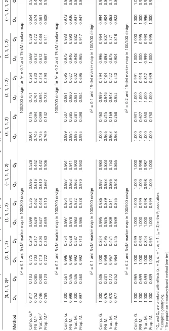
Table 5 presents the detection powers obtained by com-plete genotyping and different selective genotyping methods in the four settings under the cases of different designs, heritabilities, and marker maps. In general, the proposed method is more powerful than the PFB method and the truncated model, especially, for detecting QB in the (a1=
3,d1= 1,a2= 1,iaa= 2) setting. For example, forh2= 0.2
in the 100/200 (100/500) design, the powers of detecting QBby our proposed method are of 0.560 (0.809) and 0.498
(0.750), under 5- and 15-cM marker maps. The powers of detecting QB by the PFB method are 0.436 (0.699) and
0.385 (0.627), respectively, and the powers of detecting QB by the truncated model are 0.436 (0.593) and 0.381
(0.550), respectively. Besides, in most cases, the (proposed) modelfitting full data is more powerful than the truncated model fitting only the genotyped data, which is more evi-dent in the 100/500 design. For example, in the (a1=21,
d1= 1,a2= 1,iaa= 2) setting of the 100/500 design, the powers to detect QAand QBby the proposed (PFB) method
are 0.948 (0.933) and 0.865 (0.833), and the powers by the truncated model are 0.896 and 0.750 under h2= 0.1 and
the 5-cM marker map. Also, the detecting powers obtained by the proposed method in the 100/200 design are roughly close to those obtained by complete genotyping in the 200/ 200 design. For example, in the case of h2= 0.1 and the
5-cM marker map in the 100/200 design (200/200 design), the powers to detect QAand QBare 0.765 and 0.123 (0.817
and 0.103), 0.722 and 0.280 (0.775 and 0.249), 0.659 and 0.510 (0.699 and 0.536), and 0.667 and 0.506 (0.696 and 0.528), respectively, in the (a1= 3,d1= 1,a2= 1,iaa= 2), (a1= 2,d1= 1,a2= 1,iaa= 2), (a1= 1,d1= 1,a2= 1,iaa= 2), and (a1=21,d1= 1,a2= 1,iaa= 2) settings. Similar trends can be observed in the other cases in the 100/200 design as compared to the results from their 200/200 design (the slightly higher power with selective genotyping may be due to simulation error). It shows that our proposed method (in 100/200 design) has a better ability to maintain the similar power to complete genotyping (in 200/200 design) than the other two models (in the 100/200 design). Never-theless, depending on the (relative) sizes of the QTL, the detecting powers obtained by the selective genotyping methods in the 100/500 design are obviously lower than those obtained by complete genotyping in the 500/500 de-sign (see Table 5).
Conclusion and Discussion
The approach of selective genotyping has been widely used for the detection and validation of QTL in genetic studies (Lander and Botstein 1989; Manichaikulet al.2007; Vikram
et al.2012; Luet al.2013; Fontanesiet al.2014). Statistical QTL mapping methods developed for selective genotyping can consider either full data or only genotyping data in the
QTL analysis (Xu and Vogl 2000). When only the genotyp-ing data are used in the analysis, the truncated mixture model can be applied to the QTL analysis. If the full data are considered in the analysis, the mixture model can be readily implemented to the QTL detection. In this article, we pro-posed a novel mixture model on the basis of the multiple-QTL model for selective genotyping when full data are included in the analysis. Our proposed model attempts to use the proportions of QTL genotypes in the ungenotyped individuals, rather than the population proportions of QTL genotypes as in the PFB model, to fit the ungenotyped individuals in model construction. Consequently, as shown in this article, the proposed method has the ability to pro-vide better resolution for QTL detection, to analyze epistasis, and to deal with multiple QTL problems in selective geno-typing. In addition, we provide a version of the multiple-QTL approach for the truncated mixture model, so that QTL mapping under selective genotyping can be compared and investigated among the different models in multiple QTL conditions. Simulation results show that our proposed method is more powerful than the PFB and truncated meth-ods. Notably, under the 100/200 design, our selective genotyping method can produce roughly equivalent power to complete genotyping (the 200/200 design), and the PFB methods may have difficulty doing so. Under the 100/500 design, selective genotyping has difficulty matching com-plete genotyping (the 500/500 design) in QTL detection power, because the linkage information about QTL from the genotyped individuals is inadequate relative to that from the entire sample. Also, the analysis using full data, such as by using our proposed method, performs better than that using only genotyping data, because additional information from the ungenotyped individuals is incorporated into the analysis (Xu and Vogl 2000).
In the selective genotyping experiment, the individuals with intermediate trait values (in the central part of the trait distribution) contain less information about QTL than the extreme individuals (Lander and Botstein 1989) and are not genotyped for markers. When fitting them into the model, there is no marker to infer the genotypic distributions of the underlying QTL. As a result, the PFB methods use (fixed) genotypic distribution of QTL in the population as their ge-notypic distributions to model the ungenotyped individuals (Muranty and Goffinet 1997; Xu and Vogl 2000). However, the genotypic distribution of the QTL in these ungenotyped individuals will differ from that in the population and depends on several known and unknown factors. The known factors include the population structure and selection inten-sity. The unknown factors contain the modes (additive, dom-inance, epistasis) of QTL action, size of QTL, linkage strength between QTL. That is to say, the distribution of QTL genotype in the ungenotyped individuals is informative about these factors. On the contrary, the genotypic distribution of QTL in the population is not so informative about the factors in modeling the ungenotyped individuals, as it is equivalent to that in the ungenotyped individuals only under the null that
there is no QTL. Therefore, it is possible to gain advantage andfit better to the data from selective genotyping if a method can use the distribution of QTL genotypes in the ungenotyped individuals to model the trait values of the ungenotyped indi-viduals in model construction. Apparently, such a consideration is ignored by the PFB methods, but is taken into account in our proposed model (Equation 9). Hence, our proposed method can further improve QTL mapping under selective genotyping. The empirical threshold values for selective genotyping and complete genotyping have been found to be similar (Muranty and Goffinet 1997; Manichaikulet al.2007). We have further identified that the proposed, PFB, and truncated models have similar empirical threshold values, which may be because they are all constructed by assuming the same population genomic structure.
It is challenging to analytically explore how the differ-ence between QTL effects is affecting the efficiency of selective genotyping (relative to complete genotyping). Ronin et al. (1998) showed that the power of separating two linked QTL with different direction of effects is higher than that with the same direction under selective geno-typing, which is also validated by Kao and Zeng (2010) in complete genotyping. Senet al.(2009) found that when one or more QTL have large effects, the effectiveness can be unpredictable in their information analysis. This implies that selective genotyping may show better efficiency in QTL map-ping under some combinations of QTL parameters than un-der others, which is validated in our simulation study. Selective genotyping might be most convenient and suitable for the cases in which only one trait is targeted for selection and being analyzed in QTL mapping (Darvasi 1997). The multiple-trait analysis by including the targeted trait and its correlated traits in the model at a time can also improve the power of QTL detection due to taking into account the correlated structure of traits (Jiang and Zeng 1995; Muranty
et al. 1997; Ronin et al. 1998). When multiple traits are targeted for selective genotyping experiments, extreme indi-viduals in one trait may not be the extreme indiindi-viduals in the others, and the issues of which traits should be selected and of defining the criteria of selection have been important and discussed by several researchers (Lin and Ritland 1997; Muranty and Goffinet 1997; Murantyet al. 1997; Xu and Vogl 2000). Murantyet al.(1997) suggested using a selec-tion index combining all trait values to select the extreme individuals and then treated their index values as new single trait values in the analysis. Our method can be readily implemented to analyze the index values for multiple-trait analysis. For directly taking multiple traits into account in the analyses, the multivariate versions of the PFB model
fitting one and two QTL have been developed by Muranty
et al.(1997) and Roninet al.(1998), respectively, and the multivariate version for the truncated normal mixture model for fitting one QTL has been proposed by Xu and Vogl (2000). The multivariate version of our proposed model for directly analyzing multiple traits has not yet been con-sidered here and can be pursued on the foundation of
multivariate normal mixture model laid by Jiang and Zeng (1995), Murantyet al.(1997), Roninet al.(1998), and Xu and Vogl (2000) in future studies.
Acknowledgments
The authors are grateful to Mr. Po-Ying Chu for the discussions. We are also grateful to the associate editor and the referees for their valuable comments and suggestions. This study was supported partly by grants NSC102-2313-B-001-019 from the National Science Council, Taiwan, Republic of China.
Literature Cited
Abdel-Haleem, H., G.-J. Lee, and R. H. Boerma, 2011 Identification
of QTL for increasedfibrous roots in soybean. Theor. Appl. Genet.
122(5): 935–946.
Cohen, A. C., 1991 Truncated and Censored Samples: Theory and
Applications. Dekker, New York.
Darvasi, A., 1997 Interval-specific congenic strains (ISCS): an
ex-perimental design for mapping a QTL into a 1-centimorgan
in-terval. Mamm. Genome 8(3): 163–167.
Darvasi, A., and M. Soller, 1992 Selective genotyping for
deter-mination of linkage between a marker locus and a quantitative
trait locus. Theor. Appl. Genet. 85: 353–359.
Fontanesi, L., G. Schiavo, G. Galimberti, D. G. Calo, and V. Russo,
2014 A genome wide association study for average daily gain
in Italian Large White pigs. J. Anim. Sci. 92: 1385–1394.
Henshall, J. M., and M. E. Goddard, 1999 Multiple-trait mapping
of quantitative trait loci after selective genotyping using logistic
regression. Genetics 151: 885–894.
Jiang, C. C., and Z.-B. Zeng, 1995 Multiple trait analysis of genetic
mapping for quantitative trait loci. Genetics 140: 1111–1127.
Kao, C.-H., and H.-A. Ho, 2012 A score-statistic approach for
determin-ing threshold values in QTL mappdetermin-ing. Front. Biosci. E4: 2670–2682.
Kao, C.-H., and Z.-B. Zeng, 1997 General formulas for obtaining
the MLE and the asymptotic variance-covariance matrix in map-ping quantitative trait loci when using the EM algorithm.
Bio-metrics 53: 359–371.
Kao, C.-H., and M.-H. Zeng, 2010 An investigation of the power
for separating closely linked QTL in experimental populations.
Genet. Res. 92: 283–294.
Kao, C.-H., Z.-B. Zeng, and R. D. Teasdale, 1999 Multiple interval
mapping for quantitative trait loci. Genetics 152: 1203–1216.
Lander, E. S., and D. Botstein, 1989 Mapping mendelian factors
underlying quantitative traits using RFLP linkage maps.
Genet-ics 121: 185–199.
Lebowitz, R. J., M. Soller, and J. S. Beckmann, 1987 Trait-based
analyses for the detection of linkage between marker loci and quantitative trait loci in crosses between inbred lines. Theor.
Appl. Genet. 73: 556–562.
Lin, J. Z., and K. Ritland, 1997 Quantitative trait loci
differenti-ating the outbreedingMimulus guttatusfrom the inbreedingM.
platycalyx. Genetics 146: 1115–1121.
Little, R. J. A., and D. B. Rubin, 1987 Statistical Analysis with
Missing Data. Wiley, New York.
Lu, X., H. Wang, B. Liu, and J. Xiang, 2013 Three EST-SSR
markers associated with QTL for the growth of the clam Mere-trix mereMere-trix revealed by selective genotyping. Mar. Biotechnol.
15: 16–25.
Manichaikul, A., A. A. Palmer, ´S. Sen, and K. W. Broman,
2007 Significance thresholds for quantitative trait locus
map-ping under selective genotymap-ping. Genetics 177: 1963–1966.
Miller, A. R., N. A. Hawkins, C. E. McCollom, and J. A. Kearney,
2013 Mapping genetic modifiers of survival in a mouse model
of Dravet syndrome. Genes Brain Behav. 13: 163–172.
Muranty, H., and B. Goffinet, 1997 Selective genotyping for
loca-tion and estimaloca-tion of the effect of a quantitative trait locus.
Biometrics 53: 629–643.
Muranty, H., B. Goffinet, and F. Santi, 1997 Multitrait and
multi-population QTL search using selective genotyping. Genet. Res.
70: 259–265.
Ronin, Y. I., A. B. Korol, and J. I. Weller, 1998 Selective
genotyp-ing to detect quantitative trait loci affectgenotyp-ing multiple traits:
in-terval mapping analysis. Theor. Appl. Genet. 97: 1169–1178.
Sen, S., F. Johannes, and K. W. Broman, 2009 Selective genotyping
and phenotyping strategies in a complex trait context. Genetics
181: 1613–1626.
Vikram, P., B. P. M. Swamy, S. Dixit, H. Ahmed, M. T. S. Cruzet al.,
2012 Bulk segregant analysis: An effective approach for
map-ping consistent-effect drought grain yield QTLs in rice. Field
Crops Res. 134: 185–192.
Xu, S., and C. Vogl, 2000 Maximum likelihood analysis of
quan-titative trait loci under selective genotyping. Heredity 84: 525–
537.
Appendix
When applying the model in Equation 3 to analyze genotyping data from selective genotyping, the likelihood function is a mixture of truncated normals with different means and mixing proportions. By treating the truncated normal mixture model as an incomplete-data problem (Little and Rubin 1987), we can apply the EM algorithm to obtain the MLEs of QTL parameters. Lett1j¼ ðTL2mjÞ=sandt2j¼ ðTR2mjÞ=sbe the left and right truncation points after standardizing by their means and standard deviations. Then, we have
Uj¼ Z t1j
2NfðxÞdxþ
Z N
t2j
fðxÞdx¼Ft1j
þ12Ft2j
;
wheref() andF() denote standard normal p.d.f. and c.d.f., respectively. For illustration, we take an additive model form
QTL in the model as an example. The EM algorithm for obtaining the MLE of the parameters in the likelihood (Equation 5) is described as below. In E step, the conditional expected complete-data log-likelihood
Q
QjQðtÞ ¼X ns
i¼1
X3m
j¼1
log
0 @f
yijmj;s2
Uj pij 1 ApðtÞ
ij
¼X
ns
i¼1
X3m
j¼1
h
logf
yijmj;s2 2logUjþlog
pij
i pðtÞij
¼X
ns
i¼1
X3m
j¼1
h
logf
yijmj;s2 þlog
pij
i pðtÞij 2
Xns
i¼1
X3m
j¼1
logUjpðtÞij
is computed, wherepij’s are the posterior probabilities of QTL genotype. The last term in the right-hand side is a correction term for truncation.
The M step is to find Q(t+1) that maximize the conditional expected log-likelihood Q(Q|Q(t)). We first obtain the
derivatives of log Ujwith respect to each parameter as follows. For the effect, say ai, associated with the ith column of the genetic design matrix D(Di), the derivative is
@ @ailog
Uj¼ @ @ailog
Ft1j
þ12Ft2j
¼ð@=@aiÞ
Ft1j
þ12Ft2j
Ft1j
þ12Ft2j
¼f
t1j
ð@=@aiÞt1j2f
t2j
ð@=@aiÞt2j Ft1j
þ12Ft2j
¼f
t1j
ð@=@aiÞhTL2mj
. s
i
2ft2j
ð@=@aiÞhTR2mj
. s
i
Ft1j
þ12Ft2j
¼f
t1j
2ð1=sÞð@=@aiÞmj 2ft2j
2ð1=sÞð@=@aiÞmj
Ft1j
þ12Ft2j
¼ 2ð1=sÞ f
t1j
2ft2j
Ft1j
þ12Ft2j Dij;
whereDijis theij-entry of design matrixD. Formands2, the derivatives are
@ @mlog
Uj¼ 21 s
ft1j
2ft2j
Ft1j
þ12Ft2j
@ @s2log
Uj¼f
t1j
@@s2t1j2f
t2j
@@s2t
2j
Ft1j
þ12Ft2j
¼f
t1j
212s2hTL2mj
. s
i
2ft2j
212s2hTR2mj
. s
i
Ft1j
þ12Ft2j
¼ 2 1
2s2
ft1j
t1j2f
t2j
t2j Ft1j
þ12Ft2j ;
respectively. For simplicity in the following derivations, we define
Aj¼ f
t1j
2ft2j
Ft1j
þ12Ft2j
and Bj¼t1jf
t1j
2t2jf
t2j
Ft1j
þ12Ft2j
; j¼1;2;⋯;3m:
The partial derivatives ofQ(Q|Q(t)) with respect of each parameters are described below, For one of the QTL effect, saya1,
the derivative is
@ @a1
Q
QjQðtÞ ¼ 1 s2
h
ðY2m1nsÞ9PðtÞD1219nsPðtÞðD1#D1Þa1219nsPðtÞðD1#D2Þa22⋯
219nsPðtÞðD1#DkÞakþs19nsPðtÞðA#D1Þ
i ;
where # denotes the element-by-element product of the two same-order matrices,P¼ fpijgns33m,A¼ ðA1;A2;⋯;A3mÞ9.
The derivatives for other effects have the similar expressions. For mands2, the derivatives are @
@mQ
QjQðtÞ ¼ 1 s219ns
Y2m1ns2PðtÞDEþsPðtÞA
@ @s2Q
QjQðtÞ ¼ 1
2s4
h
ðY2m1nsÞ9ðY2m1nsÞ22ðY2m1nsÞ9PðtÞDEþE9VðtÞE2s2
ns219nsP ðtÞB i
whereB¼ ðB1;B2;⋯;B3mÞ9and
V¼
0 B B @
19nsPðD1#D1Þ 19nsPðD2#D1Þ ⋯ 19nsPðDk#D1Þ
19nsPðD1#D2Þ 19nsPðD2#D2Þ ⋯ 19nsPðDk#D2Þ
19nsPðD1#DkÞ 19nsPðD2#DkÞ ⋯ 19nsPðDk#DkÞ 1 C C A:
The solutions of the above partial derivatives can be obtained in close forms. For the effecta1,
aðtþ1 1Þ¼
Y2mðtÞ1ns
9PðtÞD
12⋯219nsPðtÞðD1#DkÞaðtÞk þsðtÞ19nsPðtÞ
AðtÞ#D
1
19nsPðtÞðD1#D1Þ
:
The solutions for the other effects have similar expressions and can be easily formulated accordingly by operating their corresponding column vectors inD. These solutions for the effects can be arranged together and expressed in matrix form as Equation 7. The solutions formands2are
mðtþ1Þ¼ 1 ns
h
19nsY2PðtÞDEðtþ1Þ þ19nssðtÞPðtÞAðtÞ i
;
s2ðtþ1Þ¼ 1 ns219nsPðtÞBðtÞ
Y2mðtþ1Þ1ns 9
Y2mðtþ1Þ1ns 22
Y2mðtþ1Þ1ns 9PðtÞDEðtþ1ÞþEðtþ1Þ9VðtÞEðtþ1Þ
: