Integrated Techno-economic and Environmental Analysis in Support of Biorefinery Technology Commercialization and Product Scheme Decision-making.

(1)

ABSTRACT

REEB, CARTER WALKER. Integrated Techno-economic and Environmental Analysis in Support of Biorefinery Technology Commercialization and Product Scheme Decision-making. (Under the direction of Richard Venditti, Stephen Kelley, Ronalds Gonzalez and Elizabeth Nichols).

The bioeconomy is a relatively new market sector comprising bio-energy, bioplastics,

biofuels, bio-based textiles and packaging, and pharmaceuticals. Government support for the bioeconomy has incentivized the production of bioproducts for companies endeavoring to bring bio-based products to market. Critical tools for predicting the commercialization feasibility of a bioproduct or biorefining scheme include process modeling and

techno-economic analysis, bench- and pilot-scale experimental results, and market analysis. Whereas financial and technical metrics are good predictors of operational and economic feasibility at commercial scale, these metrics lack the ability to quantify essential product or system utility functions as mandated for governmental incentives, which require positive socio-economic and environmental outcomes. Unfortunately, once numerous criteria are measured for scenarios and bioproducts under comparison, the complexity of subsequent scenario comparison disallows objective, normative decision-making. Decision science, specifically methodologies classified as multi-criteria decision-making analysis (MCDA) allow for systematic, objective scenario comparison via weighted single-scoring.

The objective of this research is to employ MCDA as an integrated analysis and decision-making tool to evaluate the holistic feasibility of various biorefinery conversion technologies and bioproduct schema using technological, economic, social, logistical, environmental and financial criteria. This MCDA tool may facilitate more objective decision-making for biorefinery investors and operators; the success of which will promote the continued growth of the U.S. bioeconomy. This integrated assessment will present data from many robust modeling and analysis tools and methodologies and will explore the integration of these data and methodologies to develop a clearer picture of holistic biorefinery feasibility and

conversion technology scalability for stakeholders.

(2)

conversion technologies such as gasification to mixed alcohols. In Chapters 2, 3, and 4, in-depth biomass supply system models were developed for eighteen biomass types including primary agricultural and forestry crops as well as agricultural and forestry residues in order to better measure feasibility metrics for biomass supply. Cradle-to-gate feasibility analysis was conducted as a truncated assessment of unspecified product biorefining feasibility.

Experimental weight sets were developed which weighted feasibility criteria differently in order to approximate a stakeholder’s values during decision-making. Results of this biomass supply analysis were used to select scenarios which are more likely to be feasible for cradle-to-grave analysis of biosugar, bioethanol oxygenate, fuel pellet, and transportation fuels conversion technologies and biorefining/bioprocessing scenarios.

Conversion technologies assessed herein include (a) various pretreatment options followed by enzymatic hydrolysis and distillation to biosugar (biochemical conversion, Chapter 5 and Chapter 6), (b) fast pyrolysis followed by hydrodeoxygenation, catalytic cracking, and distillation to gasoline range molecules (Chapter 7), (c) biochemical saccharification and fermentation of corn to bioethanol (Chapter 5 and Chapter 8), (d) biochemical

saccharification and fermentation of cellulosic biomass to bioethanol (Chapter 5 and Chapter 8), and (e) densification to fuel pellets for bioenergy production via combustion (Chapter 8). Outcomes of this completed research include evidence of the successful integration of disparate feasibility analysis methodologies and the identification of technologies which are most feasible and which provide the greatest utility for stakeholders. Implications of

(3)

(4)

Integrated Techno-economic and Environmental Analysis in Support of Biorefinery Technology Commercialization and Product Scheme Decision-making

by

Carter Walker Reeb

A dissertation submitted to the Graduate Faculty of North Carolina State University

in partial fulfillment of the requirements for the Degree of

Doctor of Philosophy

Forest Biomaterials

Raleigh, North Carolina

2015

APPROVED BY:

_______________________________ ______________________________

Stephen Kelley Richard Venditti

Committee Co-chair Committee Co-chair

________________________________ ________________________________

(5)

DEDICATION

(6)

BIOGRAPHY

Carter Reeb was born in Canada and moved to North Carolina in 1995 with his family. His love for the environment brought him to North Carolina State University in 2005 to study Environmental Technology and Management where he conducted independent research in biogeochemistry. He then went on to work as a project manager of environmental

remediation and industrial water treatment sites throughout the US and Canada until he returned to NC State in 2012 to pursue his Ph.D. Carter’s passion for the environment is the main driver behind his doctoral research of alternative fuels and sustainability metrics, including novel research into the integration of techno-economic analysis, environmental life cycle assessment and multi-criteria decision-making analysis. During graduate school, Carter completed an internship at Albemarle Corporation’s Heavy Oil Upgrading catalyst research and development laboratory in Houston, Texas, worked as a contract journal article editor, and co-founded Triangle Life Cycle Assessment, a consultancy implementing novel

(7)

ACKNOWLEDGMENTS

I would like to acknowledge, first and foremost, my committee co-chairs and advisers Stephen Kelley and Richard Venditti, who helped frame my work, improve my critical thinking and problem solving abilities, and guide my research interests. I learned to truly love my research during our many conversations and projects together. Your great example as scientists and as people has made graduate school a transformative experience for me. Equally, I would like to acknowledge my committee members, Elizabeth Guthrie Nichols and Ronalds Gonzalez, whose invaluable guidance and challenging questions helped me ask better questions in return. Thanks also to Richard Phillips, who has helped me immensely as I continue to learn process model development and techno-economic analysis.

I would also like to acknowledge my office mates, Jesse Daystar, Trevor Treasure, Steve Pires, Charles Grant Culbertson, Tyler Hays, Robert Radics, Neethi Rajagopalan, and Priscilla Morris, who I value greatly as colleagues and friends.

(8)

TABLE OF CONTENTS

LIST OF TABLES ... xvi

LIST OF FIGURES ... xxx

CHAPTER 1 ... 1

1. Introduction ... 1

1.1 Introduction to the Bioeconomy ... 1

1.2 Economic Drivers for the Bioeconomy ... 2

1.3 Financial Drivers for the Bioeconomy ... 5

1.4 Environmental Drivers for the Bioeconomy ... 6

1.5 Policy Drivers for the Bioeconomy... 8

1.6 Overview of Current Technologies and Bioproducts ... 14

1.7 Current Status of Commercialization Efforts... 18

1.8 Implications for Research ... 20

1.9 Biorefinery Commercialization Feasibility ... 22

1.10 Techno-economic Analysis ... 24

1.11 Environmental Life Cycle Assessment ... 27

(9)

1.11.2 Stochastic Multi-Attribute Analysis for Life Cycle Impact Assessment ... 30

1.12 Multi-Criteria Decision-making Analysis for Feasibility Analysis ... 31

1.13 Gaps in the Literature ... 31

1.14 Objectives and Research Questions ... 33

1.15 References Cited ... 36

CHAPTER 2 ... 54

2. Environmental LCA and Financial Analysis to Evaluate the Feasibility of Bio-based Sugar Feedstock Biomass Supply Globally: Part 1. Supply Chain Analysis ... 54

2.1 Abstract ... 54

2.2 Introduction ... 54

2.3 Methods ... 56

2.3.1 Feedstock Supply Chains ... 58

2.3.2 Delivered Cost ... 61

2.3.3 Life Cycle Assessment ... 61

2.4 Results and Discussion ... 62

2.4.1 Supply Chain Analysis ... 62

2.4.2 Delivered Cost ... 66

(10)

2.5 Conclusions... 76

2.6 Acknowledgements ... 77

CHAPTER 3 ... 91

3. Biomass Feasibility Case Study: Supply Chain Analysis, Delivered Cost, and Life Cycle Assessment of Oil Palm Empty Fruit Bunch Biomass for Green Chemical Production in Malaysia... 91

3.1 Abstract ... 91

3.2 Abbreviations List ... 92

3.3 Introduction ... 92

3.4 Methods ... 97

3.4.1 Goal and Scope... 97

3.4.2 Supply Chain Analysis ... 100

3.4.3 Life Cycle Assessment ... 101

3.4.4 Land Use Change ... 101

3.4.5 Delivered Cost ... 102

(11)

3.5.2 Mass Balance around a Palm Oil Extraction Facility ... 103

3.5.3 Life Cycle Inventory ... 105

3.5.4 Life Cycle Impact Assessment ... 107

3.5.5 Sensitivity Analysis ... 112

3.5.6 Delivered Cost ... 114

3.5.7 Biomass Supply Feasibility ... 119

3.5.8 Bio-based Chemical Platform Feasibility ... 119

3.6 Conclusions... 120

CHAPTER 4 ... 130

4. Environmental LCA and Financial Analysis to Evaluate the Feasibility of Bio-based Sugar Feedstock Biomass Supply Globally: Part 2. Application of Multi-Criteria Decision-making Analysis as a Method for Biomass Feedstock Comparison ... 130

4.1 Abstract ... 130

4.2 Introduction ... 131

4.3 Methods ... 133

(12)

4.3.2 Data Generation ... 140

4.3.3 Multi-criteria Decision-making Analysis ... 141

4.3.4 Sensitivity Analysis and Rank Stability ... 144

4.4.1 Unweighted Ranking Method ... 145

4.4.2 Weighted, Rank-order Distributed Scoring Method ... 146

4.4.3 Weighted, Raw Value Distributed Scoring Method ... 149

4.4.4 Ranking Stability Analysis ... 152

4.5 Conclusions... 155

CHAPTER 5 ... 161

5. Techno-economic Analysis of Various Biochemical Conversion Platforms for Biosugar Production: Trade-offs of Co-producing Energy versus Pellets for Either a Greenfield, Repurpose, or Co-location Siting Context ... 161

5.1 Abstract ... 161

5.2 Introduction ... 162

(13)

5.3.1 Study Objective ... 165

5.3.2 Feedstock Supply... 165

5.3.3 Biochemical Conversion Process ... 166

5.3.4 Process Description ... 166

5.3.5 Techno-economic Model... 166

5.4.1 Biomass Characteristics and Feedstock Cost ... 174

5.4.2 Pretreatment and Conversion Pathways ... 177

5.4.3 Siting Context ... 179

5.4.4 Co-Product Impacts ... 182

5.4.5 Summary of Conversion Pathways ... 183

5.4.6 Financial Analysis ... 185

5.4.7 Impact of Sugar Purity ... 187

5.4.8 Comparison of First and Second Generation Sugar Financials ... 189

5.4.9 Bioethanol versus Biosugar Production ... 190

(14)

5.5 Conclusions... 195

CHAPTER 6 ... 201

6. Commercial-scale Biosugar Production Using Various Biochemical Conversion Pathways, Biomass Types, Co-products, and Siting Contexts: Integrating Technical, Financial and Environmental Feasibility Analyses ... 201

6.1 Abstract ... 201

6.2 Introduction ... 202

6.3 Methods ... 206

6.4.1 Technical, Financial and Environmental Feasibility Results ... 212

6.4.2 Single Score Results ... 217

6.4.3 Statistical Analysis ... 221

6.4.4 Contribution Analysis ... 224

6.5 Conclusions... 228

(15)

7. Process Modeling of Fast Pyrolysis of Various Biomass Feedstocks for Bio-oil Production, Techno-economic analysis, Socio-economic analysis, and Life Cycle

Assessment as Compared to Fossil-based Gasoline ... 237

7.1 Abstract ... 237

7.2 Introduction ... 238

7.3 Methods ... 243

7.3.1 Modeling Methods... 245

7.3.2 Process Modeling ... 252

7.3.3 Techno-economic Analysis ... 252

7.3.4 Economic Impact Modeling... 254

7.3.5 Environmental Life Cycle Assessment ... 258

7.4.1 Results of Process Modeling in Aspen ... 263

7.4.2 Techno-economic Analysis ... 265

7.4.3 Economic Impact Analysis ... 268

7.4.4 Life Cycle Inventory ... 272

(16)

7.4.6 Comparison with Petroleum Hydrocarbons ... 278

7.4.7 Trade-off Analysis ... 280

7.5 Conclusions... 281

CHAPTER 8 ... 294

8. Comparative Analysis of the Pyrolysis, Gasification and Biochemical Conversion Pathways Commercialization Feasibility ... 294

8.1 Abstract ... 294

8.2 Introduction ... 295

8.2.1 Conversion Technologies ... 296

8.2.2 Study Objectives and Expected Outcomes... 301

8.3 Methods ... 302

8.3.1 Techno-Economic Analysis ... 302

8.3.2 Environmental Life Cycle Assessment ... 306

8.3.3 Socio-Economic Analysis ... 306

8.3.4 Multi-criteria Decision-making Analysis ... 307

(17)

8.4.1 Feasibility Metrics ... 308

8.4.2 Scenario Single-Scoring ... 320

8.4.3 Scenario Ranking ... 321

8.5 Conclusions... 326

CHAPTER 9 ... 339

9. Dissertation Summary and Conclusions ... 339

CHAPTER 10 ... 343

10. Future Work ... 343

11. Appendices ... 345

11.1 Appendix 1-1 ... 346

11.2 Appendix 2-1 ... 353

11.3 Appendix 3-1 ... 362

11.4 Appendix 3-2 ... 363

12.1 Appendix 4-1 ... 365

(18)

12.3 Appendix 5-2 ... 369

12.4 Appendix 6-1 ... 373

12.5 Appendix 6-2 ... 379

12.6 Appendix 7-1 ... 388

(19)

LIST OF TABLES

Table 1-1. U.S. fuel ethanol production by year as barrels per day (BPD) and billion gallons per year (BGPY) ... 10

Table 2-1. Overview of biomass feedstocks chosen for analysis, the country assumed for each biomass type, and the primary literature sources used for data collection ... 57

Table 2-2. Impact categories and units included in the U.S. Environmental Protection Agency’s Tool for the Reduction and Assessment of Chemical and Other

Environmental Impacts (TRACI) 2.0 method... 62

Table 2-3. Overview of biomass feedstock options chosen for analysis and relevant feedstock characteristics ... 64 Table 2-4. National annual availability estimate for each biomass feedstock type

analyzed ... 65 Table 2-5. Total delivered cost per BDMT, per metric tonne (MT) of carbohydrates and per million British Thermal Units (MBTU) embodied energy for each biomass

feedstock type by life cycle stage... 67 Table 2-6. Carbohydrate cost and content, monomeric sugar yield, and calculated feedstock cost per tonne of sugar produced for each feedstock type, based upon

(20)

Table 3-1. Composition of EFB from recent literature sources and the mean and

standard deviation of the values ... 95

Table 3-2. Malaysian CPO extraction mill average per metric tonne of CPO produced ... 105 Table 3-3. Typical data for a Malaysian palm oil plantation that produces FFB ... 106

Table 3-4. Assumptions about the empty fruit bunch loading and delivery system from the CPO extraction facility to the biorefinery, assuming 500,000 BDMT year-1

delivered, a medium-sized CPO extraction facility, and 60% EFB diversion to CHP ... 107 Table 3-5. Results of the LCA for the four allocation scenarios per BDMT of EFB to biorefinery ... 108 Table 3-6. GHG emissions, cradle-to-gate, from FFB production by life cycle stage, employing the mass allocation method ... 110 Table 3-7. The life cycle stage-specific GHG burdens (kg CO2 eq. ha-1_yr-1_{) for this study} compared against previous LCA studies of FFB production in Malaysia ... 111 Table 3-8. Comparison of EFB cradle-to-gate environmental and human health impacts per BDMT against feedstocks from Daystar et al. (2014), assuming 500,000 BDMT yr-1 delivered to a biorefinery, using Ecoinvent v2.2 data, mass allocation and the TRACI impact assessment method (Bare et al. 2002, Bare et al. 2003) ... 112 Table 3-9. Literature values of purchase price for EFB biomass ... 115

Table 3-10. The cost of loading EFB biomass into a 20-tonne truck at the CPO

(21)

Table 3-11. Transport distance (round-trip), required area, and total delivered cost per bone dry metric tonne using three different covered area assumptions for three

biorefinery scales ... 116

Table 3-12. Delivered cost of the EFB feedstock for 500,000 BDMT yr-1_{, assuming 70%} covered area, and the breakdown of delivered cost by major cost drivers. EFB delivered cost is also compared against six North American biomass feedstocks (Daystar et al.

2014) ... 118

Table 4-1. TRACI impact categories, acronyms and units (Bare et al. 2002) ... 134 Table 4-2. Scenario parameters and assumptions used for each MCDA method ... 135 Table 4-3. Aggregate uncertainty values (Frischknecht et al. 2005) as a single standard deviation from the mean (from Ecoinvent v.2.2 for each feedstock scenario model). Used in SMAA-LCIA for stochastic modeling of weighted environmental preference ... 136 Table 4-4. Biorefiner weights from Gloria et al. (2007) and the converted form used for SMAA ... 138 Table 4-5. Coefficient of variation (CV) of impact for each feedstock by impact

category, as determined by standard deviation as a percentage of the mean ... 138 Table 4-6. Cumulative environmental preference score and probability based upon the results of stochastic multi-attribute analysis coupled with life cycle impact assessment (SMAA-LCIA). A rank order of one indicates most environmentally-preferred biomass type ... 139

(22)

Table 4-8. Criterion-specific ranking and single score ranking for all eighteen biomass feedstocks based upon delivered cost, sugar yield, transport distance, harvestable months, and environmental preference. Criterions-specific rank of 18 is best, overall rank of 1 is best. ... 146

Table 4-9. Scoring of alternatives for each criterion to generate a total weighted single-score and overall ranking, using MCDA Method 2 (M2) and weight set 1 (W1). A single-score of 5 is best. A rank of 1 is the best ... 147

Table 4-10. Scoring of alternatives for each criterion to generate a total weighted score and overall ranking for MCDA Method 3 (M3), using weight set 1 (W1). A single-score of 5 is best. An overall rank of 1 is best ... 150 Table 4-11. Spearman’s rank order correlation coefficient (Sielska 2010) calculated for pairwise comparisons of the rank order ... 153 Table 5-1. Financial accounting rules used for investment analysis ... 172 Table 5-2. Contribution to net revenue for a selection of feasible scenarios, as measured by minimized MSR. All values are in 2015 U.S. dollars per metric tonne of sugar

(23)

Table 5-5. Key indicator comparison of cellulosic-derived sugars against conventional sources of corn grain and sugar cane from Latin America. Includes low cost residual biomass types: rice hulls and empty fruit bunch, and a higher sucrose-containing agricultural crop, sweet sorghum ... 189

Table 5-6. Comparison of biosugar versus bioethanol for three feedstocks. Corn grain feedstock cost of $4.00 per bushel assumed; lower than current prices. GF and PW assumed ... 191

Table 6-1. Biosugar recovery efficiency by conversion technology, gram glucose

produced/gram OD biomass ... 209 Table 6-2. Top twenty scenarios by weight set, assuming mass allocation. Minimum, average and maximum values are for all scenarios initially considered financially feasible by MSR using the $335 tonne sugar-1_{benchmark sugar price ... 218} Table 6-3. Bottom twenty scenarios that pass the financial cut-off by weight set,

assuming mass allocation. Minimum, average and maximum values are for all scenarios initially considered financially feasible by MSR using the $335 tonne sugar-1_benchmark sugar price ... 219 Table 6-4. Analysis of the contribution of multiple major cost drivers to minimum sugar revenue for “highly-feasible” scenarios. Scenarios were selected which had an average rank position of less than 25 ... 225 Table 6-5. Analysis of the contribution of major cost drivers to MSR for the “least feasible” scenarios that passed the financial cut-off. These scenarios had average ranks between 140 and 156 for all 4 weight sets ... 226

(24)

Table 6-7. Analysis of the contribution of scenario processes, inputs and outputs to GWP impacts for the lowest ranked scenarios... 228

Table 7-1. Ultimate and proximate analyses and lower and higher heating values for biomass feedstocks supplied to the fast pyrolysis system; Inputs for the pyrolysis Aspen model ... 247

Table 7-2. Process assumptions used during aspen modeling of the fast pyrolysis process ... 250 Table 7-3. Assumptions used for modeling the fast pyrolysis of biomass to bio-oil in Aspen ... 252 Table 7-4. Assumptions used for discounted cash flow rate of return (DCFROR)

analysis ... 253 Table 7-5. Process outputs and emissions as kg per hour for hydro-upgraded bio-oil production from each biomass type, assuming feedstock input rate of 500 wet metric tonnes/day ... 262 Table 7-6. Process flow data for the fast pyrolysis of biomass to bio-oil and stabilization

via reforming of bio-crude to hydrogen for hydrodeoxygenation ... 264 Table 7-7. Process flow data for the cracking and fractionation of bio-oil to

(25)

Table 7-10. Process yield values, on a per hour basis for bio-crude production, hydro-treating, and cracking to gasoline and diesel range molecules ... 265

Table 7-11. Project assumptions, calculated capital requirement, operations costs, and cost values, the local share (with impacts on direct local economic impact accounting) ... 269 Table 7-12. Direct, indirect and induced jobs created (job years per year) and economic impact for each fast pyrolysis biorefinery scenario modeled ... 269

Table 7-13. Net energy ratio values for conventional fuels, biofuels from pyrolysis and biodiesel ... 272 Table 7-14. Direct land use change (LUC) GHG impacts associated with the production of the various biomass feedstocks and crude oil for gasoline production scenarios modeled herein ... 274 Table 7-15. Global warming potential (GWP) impacts by life cycle stage, as kg CO2 equivalents per MJ of biofuel, for fast pyrolysis biomass-to-biofuel scenarios, assuming biogenic carbon emissions do not contribute towards GWP, nor is CO2 sequestered during biomass growth ... 275 Table 7-16. Financial indicators for biofuels production from crude oil and cellulosic biomass ... 278 Table 7-17. Financial, economic, environmental, technical and social feasibility

indicators for fast pyrolysis biorefining and conventional petroleum refining... 281

(26)

Table 8-2. Overview of feasibility indicators and criteria for multi-criteria decision-making ... 302

Table 8-3. Assumptions used for all discounted cash flow rate of return (DCFROR) analyses ... 304

Table 8-4. Experimental weight sets for holistic feasibility criteria, used for single-scoring and ranking of modeled scenarios ... 320

Table 8-5. Scenario values by criterion for all studied scenarios, used to develop single-scores ... 320

Table 8-6. Example of single-score calculations for the “biorefinery investor” stakeholder group, for which minimum fuel selling price, biofuel yield, economic development, jobs created and global warming potential were weighted, respectively, 50%, 20%, 20%, 5%, and 5%. MCDA Method 3 was used (see Chapter 4). A single-score of 5 is best, whereas an overall rank of 1 is best ... 321 Table 11-1. Ethanol biorefineries currently operating or under construction in the United States, feedstock, and reported vs. actual production capacity in millions of gallons per year (MGPY) ... 346 Table 11-2. Chemical composition of studied feedstock species ... 353 Table 11-3. Environmental and human health impacts for each feedstock by TRACI impact category. Units for impact categories are: GWP (kg CO2 eq.), AC (moles of H+ eq), EU (kg N eq.), EC (kg 2,4 D-eq.), OZ (kg CFC 11-eq.), PO (kg NOx eq.), CA (kg benzene eq.), NC (kg toluene eq.), and RE (kg PM2.5 eq.) ... 354

(27)

Table 11-5. Global warming potential, in kg CO2 eq. per metric tonne delivered;

contribution by chemical and life cycle stage for each biomass feedstock ... 359

Table 11-6. Parameters for rough financial analysis for bio-succinic acid production based upon literature values and feedstock costs described herein ... 360

Table 11-7. Results of rough financial analysis for bio-succinic acid production based upon the parameters in Table A5 and literature values. Margin values in red indicate negative net earnings per tonne succinic acid produced for that feedstock conversion scenario ... 361 Table 11-8. LCA processes used in openLCA to model each life cycle stage of EFB production and the database source for each record ... 362 Table 11-9. Input table for calculations of GHG emissions due to land use change from various pre-conversion scenarios to palm oil plantation land in Malaysia ... 364 Table 11-10. Experimental weight set values (W1 – W4) for the selected criteria and weight set values generated using iterative, constrained randomization as described in the methods section (CR1 – CR3). All weight sets sum to 1.00. ... 365 Table 11-11. Rank order for all method and weighting combinations and for three constrained randomization scenarios, based upon delivered cost, sugar yield, transport distance, harvestable months, and environmental preference... 366 Table 11-12. Discounted cash flow rate of return (DCFROR) analysis for greenfield pelletization of mixed southern hardwoods ... 368

(28)

Table 11-14. Rank order for all method and weighting combinations and for three constrained randomization scenarios, based upon delivered cost, sugar yield, transport distance, harvestable months, and environmental preference... 372

Table 11-15. Sugar mass yield (SY) in kg biosugar per bone-dry metric tonne of

biomass for all scenarios modeled. Green scenarios = SY > 650, Yellow scenarios = 500 < SY < 650, Red scenarios = SY < 500 ... 373

Table 11-16. Minimum sugar revenue in US$ per tonne sugar for all scenarios modeled. Green scenarios = MSR < $250, Yellow scenarios = $251 < MSR < $335, Red scenarios = MSR > $335 ... 374 Table 11-17. Global warming potential in kg CO2 eq. per tonne sugar for all scenarios modeled. Green scenarios = GWP < -2,000, Yellow scenarios = -1,999 < GWP < -1,000, Red scenarios = GWP > -999 ... 375 Table 11-18. Coefficients of Determination for the correlation coefficient of MSR versus GWP values, holding biorefining variables such as feedstock type and co-product choice constant ... 382 Table 11-19. Correlation coefficients (r) and coefficients of determination (r2_{) values for}

MSR and GWP versus major scenario characteristics (biomass type, conversion

(29)

Table 11-22. Biomass production assumptions for fast pyrolysis financial modeling ... 388 Table 11-23. Capital asset pricing model used to determine fixed capital requirements for the fast pyrolysis process ... 389

Table 11-24. Discounted cash flow rate of return (DCFROR) analysis for the fast

pyrolysis of loblolly pine to gasoline and diesel ... 391

pyrolysis of unmanaged hardwoods to gasoline and diesel ... 392

pyrolysis of switchgrass to gasoline and diesel ... 393 Table 11-27. Discounted cash flow rate of return (DCFROR) analysis for the fast

pyrolysis of corn stover to gasoline and diesel... 394 Table 11-28. Life Cycle Inventory for conversion of loblolly pine to bio-oil via fast pyrolysis ... 395 Table 11-29. Life Cycle Inventory for conversion of unmanaged hardwood to bio-oil via

fast pyrolysis ... 396 Table 11-30. Life Cycle Inventory for conversion of switchgrass to bio-oil via fast

pyrolysis ... 397 Table 11-31. Life Cycle Inventory for conversion of corn stover to bio-oil via fast

(30)

Table 11-33. Overview of results from process and discounted cash flow rate of return models for all feedstocks/conversion technologies ... 401

Table 11-34. Discounted cash flow rate of return (DCFROR) analysis for corn ethanol production, assuming 65 mgpy, a 9-month construction period, and a fuel yield of 71.9 gasoline-equivalent gallons of ethanol per dry U.S. short ton of corn grain ... 402

Table 11-35. Discounted cash flow rate of return (DCFROR) analysis for cellulosic ethanol production from loblolly pine via biochemical conversion, assuming 65 mgpy, a 36-month construction period, and a fuel yield of 35.5 gasoline-equivalent gallons of ethanol per dry U.S. short ton of biomass ... 403 Table 11-36. Discounted cash flow rate of return (DCFROR) analysis for mixed

alcohols production from loblolly pine via indirect gasification, assuming 65 mgpy, a 36-month construction period, and a fuel yield of 66.9 gasoline-equivalent gallons of ethanol per dry U.S. short ton of biomass ... 404 Table 11-37. Discounted cash flow rate of return (DCFROR) analysis for liquid

hydrocarbon fuels production from loblolly pine via fast pyrolysis and

(31)

Table 11-39. Discounted cash flow rate of return (DCFROR) analysis for mixed alcohols production from unmanaged hardwood via indirect gasification, assuming 65 mgpy, a 36-month construction period, and a fuel yield of 66.9 gasoline-equivalent gallons of ethanol per dry U.S. short ton of biomass ... 407

Table 11-40. Discounted cash flow rate of return (DCFROR) analysis for liquid hydrocarbon fuels production from unmanaged hardwood via fast pyrolysis and hydrodeoxygenation, assuming 65 mgpy, a 36-month construction period, and a fuel yield of 52.4 gasoline-equivalent gallons of bio-oil per dry U.S. short ton of biomass ... 408 Table 11-41. Discounted cash flow rate of return (DCFROR) analysis for cellulosic ethanol production from switchgrass via biochemical conversion, assuming 65 mgpy, a 36-month construction period, and a fuel yield of 43.1 gasoline-equivalent gallons of ethanol per dry U.S. short ton of biomass ... 409 Table 11-42. Discounted cash flow rate of return (DCFROR) analysis for mixed

alcohols production from switchgrass via indirect gasification, assuming 65 mgpy, a 36-month construction period, and a fuel yield of 64.2 gasoline-equivalent gallons of

ethanol per dry U.S. short ton of biomass ... 410 Table 11-43. Discounted cash flow rate of return (DCFROR) analysis for liquid

hydrocarbon fuels production from switchgrass via fast pyrolysis and

(32)

Table 11-45. Discounted cash flow rate of return (DCFROR) analysis for mixed

alcohols production from corn stover via indirect gasification, assuming 65 mgpy, a 36-month construction period, and a fuel yield of 61.9 gasoline-equivalent gallons of

ethanol per dry U.S. short ton of biomass ... 413

Table 11-46. Discounted cash flow rate of return (DCFROR) analysis for liquid hydrocarbon fuels production from corn stover via fast pyrolysis and

hydrodeoxygenation, assuming 65 mgpy, a 36-month construction period, and a fuel yield of 42.6 gasoline-equivalent gallons of ethanol per dry U.S. short ton of biomass ... 414 Table 11-47. Discounted cash flow rate of return (DCFROR) analysis for conventional petroleum refining in North Carolina, at a crude oil charge rate of 6,000 barrels per day, a yield of 201 gasoline-equivalent gallons of transport fuel per U.S. short ton of crude oil, assuming 2% inflation, 35% tax rate, crude oil price of $55 per barrel, 36 month construction term, ten year investment term, debt interest rate of 8% and a debt-to-equity ratio of 40%/60% ... 415 Table 11-48. Rank position for all scenarios and all weight sets employed, assuming equal distribution of weighted criterion-specific scores across the quintile weight space ... 418 Table 11-49. Rank position for all scenarios and all weight sets employed, assuming distribution of weighted criterion-specific scores across the quintile weight space by magnitude ... 418

(33)

LIST OF FIGURES

Figure 1-1. Change in U.S. price and importation volume of crude oil, 2009-2014 (EIA 2015) ... 3 Figure 1-2. U.S. crude oil imports and extraction rates, 2009-2014 (EIA 2015) ... 3

Figure 1-3. Crude oil and bio-crude production in the US and Canada, 2009–2014 (EIA 2015) ... 4

Figure 1-4. Production cost per gallon of biofuels, levelized by facility size and to 2015 dollars ... 5

Figure 1-5. Biofuel volumes mandated by RFS2 (NRC 2011). Note: all volumes (except for biodiesel) are in billions of ethanol-equivalent gallons ... 9 Figure 1-6. U.S. fuel ethanol imports and exports in millions of gallons per year

(MGPY). Data from the Energy Information Administration (2015) ... 10 Figure 1-7. U.S. fuel ethanol imports from Brazil in million gallons per year (MGPY). From the Energy Information Administration (2015) ... 11 Figure 1-8. CAFE fuel economy requirements by model year and wheelbase footprint ... 12 Figure 1-9. U.S. ethanol production, renewable fuels standard targets for each year, and use of renewable identification numbers (RINs) to achieve the RFS target where

necessary. All production values are billions of gallons per year (from EIA 2013) ... 13

(34)

Figure 1-11. Annual net revenues for the most promising second-generation biofuels companies... 19

Figure 1-12. Representation of the “Valley of Death”, which typifies the innovation stage-gate process of technology and process scale-up (Hurden and Rimmer 2015) ... 21

Figure 2-1. Supply system scope and boundary for corn grain, corn syrup, corn stover, and Genera corn stover ... 58

Figure 2-2. Supply system scope and boundary for softwoods, US eucalyptus, and Brazilian eucalyptus. Adapted from Daystar et al. (2014) ... 59

(35)

Figure 2-9. Biomass feedstock delivered cost per MT carbohydrates and major cost drivers for each biomass feedstock, assuming 500,000 BDMT yr-1_{. If biomass purchase} price is not included, it is equal to establishment, maintenance and harvest costs for that biomass ... 68

Figure 2-10. Global warming potential (GWP) per BDMT biomass delivered and the life cycle stage-wise contributions. Note the y-axis has an axis break at -1,000 kg CO2 eq and two scales, for above and below the origin. The positive bars indicate actual non-biogenic emissions based GWP impact without sequestration ... 74

Figure 2-11. TRACI impact assessment results for all feedstocks cradle-to-gate. Larger squares indicate higher environmental impact within a category per BDMT. Raw TRACI impact values in table form can be found in Appendix 2-1 Table 11-3. For the GWP impact category all of the scenario values were negative; in this plot the size of the square is larger for those scenarios with larger net GWP impacts ... 75 Figure 3-1. Estimated annual available quantity of EFB, in metric tonnes per year for a bio-sugar platform in Malaysia (MPOB 2014) ... 96 Figure 3-2. Life cycle stages and major inputs and outputs for the palm oil FFB and EFB production and delivery systems... 100 Figure 3-3. A mass balance for the crude palm oil extraction process in Malaysia

whereby EFB is co-produced as a waste product and utilized to some extent for combined heat and power (CHP). EFB to the biorefinery currently is either land

(36)

Figure 3-4. Impacts using TRACI for the three allocation scenarios normalized to 100% of the largest impact for each impact category, assuming 500,000 BDMT year-1

delivered to a biorefinery from a medium-sized CPO extraction facility in Malaysia. Mass allocation assigns 26.9% and economic allocation assigns 1.67% of the FFB production to the EFB to the biorefinery. GW = global warming impact; AC = acidification; EU = eutrophication; EC = ecotoxicity; OZ = ozone depletion; PO = photochemical oxidation; CA = carcinogenics; NC = non-carcinogenics; RE =

respiratory effects. ... 109

Figure 3-5. The sensitivity of net GHG burdens (kg CO2 eq. BDMT-1_{) to changes in} major study assumptions ... 113 Figure 4-1. Graphic representation of the combined feasibility assessment method for n biomass alternatives and application of weighting values for m criteria during the multi-criteria decision-making ranking process ... 134 Figure 4-2. Probability distribution function of each TRACI impact factor used to determine environmental preference single-score. Frequency is the probability (y-axis) that a TRACI impact category will have a particular weight contribution in % to the net environmental preference score (x-axis) is shown ... 137 Figure 4-3. Multi-criteria weighted decision making cumulative preference scores by feedstock option. Weighting values were 30% delivered cost, 25% sugar yield, 20% transportation distance, 15% harvestable months, and 10% environmental preference ... 148 Figure 4-4. Cumulative preference scores, distributed for each criterion across a

(37)

Figure 5-1. Schematic representation of the process model, supply chain model, techno-economic model and life cycle environmental impacts model integration approach for the biosugar commercialization feasibility project (Phillips 2014) ... 164

Figure 5-2. Generic flowsheet of biomass-to-biosugar process. Co-product can be excess power, fuel pellets or animal feed (for corn grain scenarios) ... 168

Figure 5-3. Delivered cost per BDT of biomass divided by % carbohydrate equals the “cost per BDT carbohydrate”. Red = agricultural residues; green = purpose-grown crops; yellow = woody biomass ... 175 Figure 5-4. Carbohydrate content of the biomass types modeled in this study. No

difference in content of eucalyptus between USA and Latin America is assumed; likewise for sugar cane between Latin America and Southeast Asia. Red = agricultural residues; green = purpose-grown crops; yellow = woody biomass ... 175 Figure 5-5. Carbohydrate recovery (monomeric sugars produced per tonne of sugars in the original biomass) for dilute acid and autohydrolysis pretreatments. Note: dilute acid pretreatment and autohydrolysis pretreatment were not found to be feasible for sweet sorghum and rice hulls, respectively, and are not reported here ... 178 Figure 5-6. Relative fuel values of collected materials, $ per GJ in the most common application. “Carbohydrate” is the market price of glucose/fuel value of glucose ... 179

Figure 5-7. Influence of siting context on total installed capital (TIC) of autohydrolysis of mixed southern hardwoods per tonne sugar produced. Red = GF = greenfield, yellow = CL = co-location, green = RP = repurpose. PW = power sales from residue and FP = fuel pellets from residue ... 180

(38)

Figure 5-9. Sugar product purity of the options herein considered most financially feasible ... 188

Figure 5-10. Impact of the price per bushel of corn grain on the economics of sugar production, with comparison to autohydrolysis of hardwood in a greenfield context co-produced with fuel pellets ... 192

Figure 5-11. Sensitivity of a) SS-AH-FP-CL, b) HW-DA-FP-CL and c) LP-SCW80%-FP-CL to changes in biosugar production capacity, biomass price, Capex per annual tonne, sugar price per tonne, pellet selling price, and enzyme price. Note: values on the x-axes represent the percent change in cost drivers from baseline value ... 193 Figure 6-1. Overview of scenario parameters and feasibility metrics considered for biosugar production models ... 208 Figure 6-2. Distribution of scenarios by feasibility metrics, including sugar mass yield (SY) as kg sugar BDMT-1_{, minimum sugar revenue (MSR) as US$ tonne}-1_{sugar, and} global warming potential (GWP) as kg CO2 eq. tonne-1_{sugar. Red lines indicate past,} present and projected 2025 global sugar prices ... 214 Figure 6-3. Distribution of scenario single-scores for all scenarios initially considered feasible by an MSR value less than the $335 metric tonne-1_{biosugar using mass}

allocation for GWP for different weight sets ... 218 Figure 6-4. GWP and MSR ranges for scenarios modeled, organized by feedstock type ... 222 Figure 6-5. MSR and GWP values, assuming system expansion, for biorefining

(39)

Figure 7-1. General process overview for fast pyrolysis of lignocellulosic biomass to fuels... 241

Figure 7-2. Diagram of integrated techno-economic, socio-economic, and environmental life cycle analyses as feasibility assessment approach ... 244

Figure 7-3. Process depiction for mass and energy flow through the fast pyrolysis process, from Jones et al. (2013) ... 246

Figure 7-4. Study parameters which most impact the financial feasibility of biorefining (adapted from Hytönen and Stuart 2011) ... 253

(40)

Figure 7-11. Sensitivity of economic impact to various scenario parameters ... 271 Figure 7-12. Cradle-to-grave global warming potential impacts for fast pyrolysis of biomass to transport fuels, as kg CO2 eq. per MJ fuel. Biomass supply impacts included in Fast Pyrolysis life cycle stage and assumed to be offset by emissions during

conversion, storage, and combustion. Gasoline impacts modeled in GREET (DOE 2015) ... 276 Figure 7-13. Cradle-to-grave global warming potential (GWP) impacts for fast

pyrolysis of different biomass types and their percent reduction as compared to

(41)

Figure 8-5. Internal rate of return from projected cash flows, discounted using a 15% hurdle rate, and fuel production costs, as 2015 dollars per gallon of gasoline equivalent fuel (GGE)... 310

Figure 8-6. Change in net present value (NPV, 2015 US$) with change in hurdle rate for a selection of biorefinery scenarios ... 310

Figure 8-7. Reported cost of different biofuels from the literature in US$ per gallon fuel produced. Fuel costs presented assume different dollar years and energy densities ... 311

Figure 8-8. Levelized cost of fuel (LCOF) in 2015 US$ per gallon fuel produced. Black column represents gasoline, red columns represent biofuels production costs for

scenarios modeled herein. A detailed list of these scenarios is included in Appendix 8-1. ... 313 Figure 8-9. Levelized cost of fuel (LCOF) and plant capacity for biofuels production scenarios from literature, adjusted for inflation to 2015 US$ per gallon of gasoline equivalents (GGE) ... 314 Figure 8-10. Average direct, indirect and induced local economic development impacts of biorefining and petroleum refining scenarios per project year ... 315 Figure 8-11. Global warming potential impacts of biofuels, as compared to conventional fossil-fuel (kg CO2 eq. per MJ fuel) ... 316 Figure 8-12. Biofuels conversion yield values, in gallons of gasoline equivalent (GGE) fuel per oven-dry US short ton of biomass for biorefinery scenarios modeled ... 317

(42)

Figure 8-14. Rank order of single-scores for the biorefinery investor weight set and contribution of each feasibility indicator to single-score. Weight values for MFSP, yield, economic development, jobs created, and global warming potential were, respectively, 50%, 20%, 5%, 20%, and 5%. A single-score of 5 is best, a rank order of 1 (most left-hand alternative) is best... 322

Figure 8-15. Range of rank positions for each conversion scenario as weight set changes, using MCDA Method 2. Rank of 1 is most preferred ... 324

Figure 8-16. Range of rank positions for each conversion scenario as weight set changes, using MCDA Method 3. Rank of 1 is most preferred ... 325 Figure 11-1. Mass balance of the corn grain, corn syrup, and corn stover co-production system ... 356 Figure 11-2. TRACI impacts normalized to 100% of the greatest impact for each

category ... 357 Figure 11-3. Global warming contribution analysis for feedstock production and

delivery per bone-dry metric tonne of biomass delivered; biomass growth is not

included ... 358 Figure 11-4. Global warming contribution analysis for feedstock production and

delivery per metric tonne of biosugar produced; biomass growth is included here ... 358 Figure 11-5. Process flow diagram of a greenfield biorefinery scenario for the

production of fuel pellets from mixed southern hardwoods ... 367

Figure 11-6. Process flow diagram of a greenfield biorefinery scenario for the

(43)

Figure 11-7. Free cash flow over the financial lifetime of the greenfield cellulosic ethanol biorefinery scenario, assuming 500,000 bone-dry metric tonnes/year of mixed southern hardwood as feedstock and co-producing fuel pellets ... 371

Figure 11-8. Future value of net revenues by investment term (year) over the lifetime of a greenfield cellulosic ethanol biorefinery, assuming 500,000 bone-dry metric

tonnes/year of mixed southern hardwood as feedstock and co-producing fuel pellets. 371

Figure 11-9. Scenario single-scores, in descending order for all scenarios which passed the $335 per tonne financial cut-off. A weight set of 20/6/20 was used for SY/MSR/GWP and system expansion was used for calculating global warming potential... 376 Figure 11-10. Scenario single-scores, in descending order for all scenarios which passed the $335 per tonne financial cut-off. A weight set of 5/80/15 was used for SY/MSR/GWP and system expansion was used for calculating global warming potential... 377 Figure 11-11. Sugar pricing model, historic values until 2015 (year-to-date) and

projected under uncertainty to 2030 ... 378 Figure 11-12. Scatter plot of global warming potential (GWP) versus minimum sugar revenue (MSR) for all scenarios studied, assuming mass allocation of GWP burdens by scenario-specific mass allocation ratio. Blue box identified scenarios which are most preferred for both GWP and MSR ... 379 Figure 11-13. Scatter plot of global warming potential (GWP) versus minimum sugar revenue (MSR) for all scenarios studied, assuming system expansion to account for co-product GWP burdens ... 380

(44)

Figure 11-15. Scatter plot of global warming potential (GWP) versus minimum sugar revenue (MSR) for all scenarios studied, assuming system expansion to account for co-product GWP burdens ... 381

Figure 11-16. Distribution of SY, MSR and GWP, including mean values (center line of box and whisker plots), 1st_{and 3}rd_{quartile markers (outside lines of box and whisker} plots), and minimum and maximum (error bars) ... 384

(45)

CHAPTER 1

1. Introduction

A bioproduct is any saleable good which, being derived from recently living plant matter, can be thought of as a renewable alternative to corresponding fossil-based products, assuming use of the renewable product offsets actual production and use of the fossil-based product. Unlike fossil-based products, bioproducts sequester, at least temporarily, carbon from the atmosphere, contributing to the net reduction in greenhouse gases in the atmosphere,

anthropogenic gases which research suggests have accelerated global climate change (IPCC 2007). To date, bioproduct commercialization has been met with mixed results. Unintended consequences such as market overshoot, project financial insolvency, negative net fossil energy ratios, and environmental trade-offs may have contributed to commercialization failure in the past.

In order to understand the potential for the commercialization of various bioproducts in the modern bioeconomy, it is critical to understand the major drivers for the bioeconomy. The purpose of this dissertation research is to predict the feasibility of various

pre-commercialized bioproducts and biorefinery scenarios using process modeling, techno-economic analysis, microtechno-economic models and environmental life cycle assessment. Results of this research may help decision-makers predict the critical characteristics of holistic feasibility and select biorefinery technologies and products that will return the promised financial rewards and reduce environmental impacts.

1.1Introduction to the Bioeconomy

(46)

fungible (nominal quality) and economically viable (financially competitive) as compared to the non-renewable product being displaced.

The natural development of the modern bioeconomy has come about in response to perceived economic, environmental, societal and political utility for those decision-makers investing money in research & development and commercializing products within the bioeconomy. 1.2Economic Drivers for the Bioeconomy

In the fifty years from 1961 to 2011, annual electrical energy use in the United States increased by approximately 112%, from 45.74 Quadrillion British Thermal Units (BTU) to 97.16 Quadrillion BTU (EIA 2012). Over this same time-frame, liquid transportation fuel usage increased by approximately 96%, an increase from 9.7 million to 19.2 million barrels of petroleum consumed per day (Clement and Schultz 2011, EIA 2012). Various phenomena contributed to the increase in energy and transportation fuel use, but the most obvious are the increase in standard of living, an approximate 5% increase in people living in urban areas, and a greater than 100% increase in gross domestic product (GDP) and the resulting rise in collective buying power in the US (Clement and Schultz 2011). At the same time that energy use has increased dramatically, the percentage of the US energy consumption portfolio that is considered “renewable” has only increased by 0.93%, from 6.49% of the total energy

consumption to 7.42%. Over the fifty-year period from 1961 – 2011, total energy

(47)

Figure 1-1. Change in U.S. price and importation volume of crude oil, 2009-2014 (EIA 2015)

In addition, while crude imports have dropped since 2009, U.S. crude extraction has increased over the same period, partially meeting the increased demand for petroleum products and transport fuels in the U.S. as importation declines, Figure 1-2.

(48)

If US crude production is increasing but still not meeting US transportation fuel demand, the decline in imports of crude oil must be met somewhere else. Canadian oil sands crude and biomass to crude have, in fact, increased since 2009, Figure 1-3.

Figure 1-3. Crude oil and bio-crude production in the US and Canada, 2009–2014 (EIA 2015)

(49)

Clearly the economic recession in the U.S. in 2008/2009 greatly impacted the price of oil, the consumption of goods, the rate of inflation/deflation, the value of the dollar, and many other factors which has led the U.S. government and businesses to prioritize energy independence, economic development, and the creation of jobs.

1.3Financial Drivers for the Bioeconomy

One of the greatest drivers for the bioeconomy is the individual decisions that firms make about biorefinery investments and bioproduct commercialization. Assuming a bioproduct is truly equivalent to the fossil-based conventional product equivalent, a firm is only

incentivized to invest in a commercial-scale biorefinery if the project exceeds the firms hurdle rate. If alternative investment options are projected to return 8-12%, and accounting for the increased risk associated with non-demonstrated conversion technologies, a firm may require a 15% discount rate to invest.

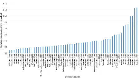
Past studies have investigated the techno-economic feasibility as measured by minimum sugar revenue (MSR) or fuel production cost, Figure 1-4.

(50)

For more analysis of biofuels production costs and cost levelization, see Section 8.3. From this survey of past biofuels techno-economic studies, levelized by facility size and to 2015 dollars using the consumer price index (see Section 8.3), the majority of studies (60%) show a production cost of less than $3.50, 38% report a production cost of less than $2.50, and only 9% report a production cost of less than $1.50. As currently reported, this means that the majority of biofuels technologies and product are not competitive against a tax-free production cost of $2.20 per gallon of gasoline in 2015 dollars (EIA 2015).

Individual firms may not always act “rationally” in economic terms, nor is it possible to perfectly predict an investor’s decision-making process with regards to perceived vs. actual technological risk and future market capacity. If a firm does not act rationally with respect to investment decisions and the emerging biofuels and bioenergy technologies and markets, it may not be helpful to calculate firm-level financial feasibility for various bioproducts and biorefinery technologies. On the other hand, “the market”, the field of possible investors, en

masse, has been described as being more economically rational. In terms of predicting the

level of participation of the whole field of investors in such a potentially-lucrative market, firm-level financial feasibility analysis is actually quite helpful for predicting the enticement necessary (hurdle rate required) for investor participation.

1.4Environmental Drivers for the Bioeconomy

As energy use has been increasing rapidly over this fifty-year period, renewable energy usage has been increasing at an increased rate of 282%, representing a total energy share of 9% in 2011 (EIA 2012). Despite an increase in the share of the energy market that is renewable, net fossil energy use has continued to increase, resulting in a net increase in CO2 and other

greenhouse gas (GHG) emissions. This is significant because many studies have been conducted which suggest that anthropogenic GHG emissions are accelerating global climate change and warming trends (IPCC 2007, Oreskes 2007, Solomon et al. 2009). As evidence continues to point towards anthropogenic sources of carbon dioxide and other GHG

(51)

reduction for climate change mitigation has led to increased innovation within the liquid transportation fuels field of research.

It has been suggested that renewable energy and transportation fuel technologies could significantly reduce the net environmental impact of energy use (Hoekman 2009, Banerjee et al. 2010, Repo et al. 2012, IPCC 2012). Traditionally renewable fuels included nuclear energy, photovoltaic arrays for capturing and converting solar energy, wind turbines, and more recently, liquid biofuel from corn and grains (Brown et al. 2000, Jungbluth et al. 2004, Turner et al. 2011). Convergence of policy, economic and market drivers has resulted in an increase in interest in biofuel as a renewable energy source for reduction of environmental impacts, increase in energy independence, jobs creation, and an increase in energy diversity and security.

Certainly the increase in renewable energy as part of the U.S. energy portfolio should be promoted, however as each of the first-generation biofuels technologies has been further developed and studied, negative environmental or economic aspects of the technology have been uncovered which has led to cautious commercialization or, in some cases, to shelving of the technology (Pimentel and Patzek 2005, Pineiro et al. 2009, de Vries et al. 2010, Feng et al. 2010). One such technology, the commercialization of which has slowed recently is corn grain-based bioethanol production via thermal hydrolysis of starches and fermentation of resulting monomeric saccharides. As it became more evident that there are serious concerns about environmental feasibility and the ethicality of reducing food stock for first-generation biofuels from corn grain and soybeans, research has shifted to various conversion pathways for non-food lignocellulosic biomass-to-biofuels (second-generation) and algae-to-biofuels (third-generation) (Phillips et al. 2007, Oliver et al. 2009, Lindquist et al. 2010, Singh et al. 2010).

(52)

emissions, and regulations that dis-incentivize products and services which either increase emissions over time or exceed an absolute emission limit. Public policies specific to the creation and use of second-generation biofuels (biofuels policies) have also been adopted and updated iteratively as further research has been conducted. This group of relevant policies can be categorized as either economic, environmental, or energy security policies.

The Southern United States has been suggested as a possible wood basket for cellulosic biofuels due to current elevated tree density, environmental conditions which suggest continued increases in productivity and yield, and an existing supply chain infrastructure which removes some of the initial cost and supply chain risk for biorefiners (Wright 2006, Johnson et al. 2007, Galik et al. 2009, Krishnakumar and Ileleji 2010, Larson et al. 2010, Miao et al. 2012). Therefore, research related to second-generation biofuels should focus heavily on biomass production and implementation of biofuels technologies in the Southern US.

1.5Policy Drivers for the Bioeconomy

Despite a recent decline in fossil fuel prices here in the U.S., issues with respect to energy security and independence, the depletion of finite resources such as crude oil and natural gas, and the environmental impacts of non-renewable energy sources still exist for these fuel types and downstream products. The Energy Policy Act of 2005 (EPAct) and Energy Independence and Security Act of 2007 (EISA) were established and implemented and the Renewable Fuels Standards (RFS) as a result of these ongoing concerns.

(53)

RFS2 requires 35 billion gallons of biofuel be produced and blended with gasoline and 1 billion gallons of biodiesel be produced annually by 2022; a 15 billion gallon subsidy cap has been enacted for corn-based biofuel, the balance which must consist of ‘Advanced Biofuel’ and ‘Cellulosic Biofuel’, no less than 16 billion gallons deriving from cellulosic material (Figure 1-5).

Figure 1-5. Biofuel volumes mandated by RFS2 (NRC 2011). Note: all volumes (except for biodiesel) are in billions of ethanol-equivalent gallons

(54)

Table 1-1. U.S. fuel ethanol production by year as barrels per day (BPD) and billion gallons per year (BGPY)

Source: EIA 2015

This continued increase in ethanol production may be caused by an increase in hybrid vehicles which can accommodate greater than 10% (v.b.) ethanol, or by a large spike in fuel ethanol exports from 5 to 14 BGPY between 2010 and 2011, Figure 1-6, and a downturn in fuel ethanol importation, Figure 1-7.

Figure 1-6. U.S. fuel ethanol imports and exports in millions of gallons per year (MGPY). Data from the Energy Information Administration (2015)

Year BPD BGPY

2009 713,083 10.9

2010 867,417 13.3

2011 908,500 13.9

2012 860,250 13.2

2013 866,667 13.3

2014 933,417 14.3

(55)

Figure 1-7. U.S. fuel ethanol imports from Brazil in million gallons per year (MGPY). From the Energy Information Administration (2015)

The EISA also authorized $25 Million in grants for research and development pertaining to cellulosic conversion technologies and repurposing of corn-grain ethanol (first-generation) conversion facilities for cellulosic ethanol (second-generation) production (Pub. L. 110-140). An additional $125 Million was authorized for training workers for new green jobs, including for advanced biofuels production.

The biofuel classifications such as ‘advanced biofuel’ and ‘cellulosic biofuel’ are defined by the EISA and enforced by the U.S. EPA. These categories are defined by percent GHG reductions as compared to conventional fossil fuel using the life cycle assessment (LCA) method. ‘Advanced biofuel’ requires a 50% reduction of GHGs across the life cycle as compared to fossil-fuel and the only feedstock expressly excluded is corn-grain. ‘Cellulosic biofuel’ refers to alcohols from cellulosic biomass and a 60% GHG reduction from fossil-fuel is mandated (Leggett et al. 2007, Sissine 2007, Szulczyk et al. 2010, McPhail et al. 2011, Mullins et al. 2011, Winters 2011, Slating et al. 2012).

(56)

ft2 (Sissine 2007, Yacobucci et al. 2007). The 2015 fleet average requirement for light-duty transport vehicles is currently 38 MPG at a 45 ft2 wheel footprint (Figure 1-8).

Figure 1-8. CAFE fuel economy requirements by model year and wheelbase footprint

If the CAFE standard is not met for a particular vehicle manufacturer a tax per vehicle is implemented which, in theory, should incentive the production of flexible-fuel vehicles which are able to utilize a higher ethanol-gasoline ratio blend (Urbanchuk 2006). This was intended to broaden the market for bioethanol, particularly (in light of the 15 billion gallon cap under RFS2) cellulosic ethanol. Unfortunately, the majority of vehicles ten years after the first RFS was enacted still have a 10-15% technological blend-wall. Instead, auto

(57)

production for cellulosic biofuel in the U.S. was determined by the EPA with guidance from the Energy Information Administration (EIA). Kumarappan (2011) suggests that to meet the 21 billion gallons/year mandated production limit for cellulosic biofuel production by 2022, a feedstock quantity of 220-300 million tons of cellulosic biomass is needed, which is well within the estimated available biomass quantity (500+ million tons) in the U.S.

Due to the fact that no annual ethanol-equivalent gallons of mandated biofuels production has been met by fossil fuel manufacturers which are required to meet production quantities, the EPA’s Moderated Transaction System (EMTS) will be used to track the sale of RINs to obligated parties trying to meet the volumetric production mandate. If an obligated party does not purchase RINs or biofuel production wavier credits they are fined for non-compliance (McPhail et al. 2011, Schnepf and Yacobucci 2012). In 2010 the average price for biodiesel RINs was $1.56 per gallon-RIN, which dropped to $1.13 per gallon-RIN in 2011. Despite this relatively high price for biodiesel RINs, the price for cellulosic RINs has traditionally been quite low, often as low as $0.03 per gallon-RIN in 2011. The RFS2 required 800 million gallons of biodiesel production in 2011 (Pub. L. 109-58), which was exceeded; approximately 1.1 billion gallons were actually produced. The volumetric requirements for biodiesel for 2012 increased to 1.00 BGY and increased again to 1.28 BGY for 2013 (EIA 2012, EPA 2012). In fact, ethanol production in the US has exceeded RFS targets each year from 2009 – 2013, Figure 1-9.

(58)

It is evident that biofuels research and production has been incentivized by the economic implications of these policies, with commercialization often outstripping technology readiness (Juday 2011, Adusumilli and Leidner 2014, Evans 2015). Combined incentives from a guaranteed market, accelerated asset depreciation, tax breaks, and other incentives represents a substantial financial benefit for biorefiners. Many companies, drawn by the promise of volumetric production incentives, have invested heavily alongside federal and state funding in commercialization of first-, second-, and third-generation biorefineries. Despite the recent market stabilization and price drop for bioethanol, the collapse of the Chicago carbon market, and other seemingly problematic causes of the federally-incentivized biofuel commercialization effort, many countries have had an even more difficult time

commercializing these technologies (Klaphake and Sasada 2010).

After a rush to invest in bioethanol production from corn grain occurred in the Midwestern US over the past decade or so, production capacity quickly exceeded the blend-wall

constrained demand for ethanol as an oxygenation additive for blended gasoline (E10). Many companies, with millions or hundreds of millions in sunk capital divested quickly or closed their door. Production volumes stabilized and few additional investments were made to bring new first-generation biorefineries on-line alongside remaining market participants. This has led to the expiry of many of the relevant biofuels policies, an increase in the cautiousness with which investors enter second- and third-generation markets, and to the realization that non-ethanol second-generation biofuels need to be researched further.

1.6Overview of Current Technologies and Bioproducts

There exist many different second-generation biofuel conversion platforms and product schemes, however the most notable are biochemical conversion to ethanol via enzymatic hydrolysis (El-Ahmady El-Naggar et al. 2014) accompanied by various pretreatment

methods (Alvira et al. 2010), indirect gasification to synthesis gas (Daystar et al. 2012, Dutta

et al. 2014) and mixed alcohol production via catalysis (Phillips 2007), and fast pyrolysis

liquefaction followed by hydrodeoxygenation (HDO) for stable bio-crude production (Jones