Integrated Volt/Var Control on Smart Distribution Systems

ABSTRACT

SHI, YUE. Integrated Volt/Var Control on Smart Distribution Systems. (Under the direction of Dr. Mesut Baran).

This study investigates the integrated Volt/Var Control (VVC) on smart distribution systems with PV penetration.

First, a two-phase VVC method is proposed to solve the Volt/Var Optimization (VVO) problem efficiently by decoupling the VVO problem into voltage problem and Var problem. In Phase I, a search based approach is used to find the optimal tap position setting for voltage regulation devices, such as load tap changer (LTC) and voltage regulator (VR). Phase II adopts the gradient based approach to determine the optimal Var injection of smart PV inverters, or solid state transformers (SST) such that the system power loss is minimized. To facilitate the coordination between the conventional slow-acting VVC devices (e.g. LTC and VR) and the fast-acting VVC devices (e.g. smart inverter and SST), a new coordinated VVC method is proposed based on the two-phase method. The proposed coordinated VVC scheme assigns the voltage problem and Var problem at two control levels. The first level uses LTC and VR to adjust the voltage level on the circuit to keep the voltages along the circuit within the range desired. The second level determines Var support needed from smart inverters or SSTs to smooth the fast voltage variations while providing effective power factor correction to keep the system power losses at minimum. For real-time implementation

purpose, a master-slave based decentralized control architecture is introduced to fit the proposed VVC methods.

VVC is more practical since it can reduce the excess operations of conventional VVC devices due to the variability of PV generation. Simulation results also show the

computational efficiency of the methods. In this dissertation, accomplishment of real-time VVC on an Hardware-In-the-Loop system and Green Energy Hub system will also be presented.

Since the proposed methods are model-based approach, load modeling for VVC in smart distribution systems is also discussed in this work. A real-time load parameter estimation approach is proposed to facilitate real-time VVC such that the VVC application has knowledge of a more accurate load model and monitors the real-time performance of VVC.

Integrated Volt/Var Control on Smart Distribution Systems

by Yue Shi

A dissertation submitted to the Graduate Faculty of North Carolina State University

in partial fulfillment of the requirements for the degree of

Doctor of Philosophy

Electrical Engineering

Raleigh, North Carolina 2018

APPROVED BY:

_______________________________ _______________________________

Dr. Mesut Baran Dr. Ning Lu

Committee Chair

DEDICATION TO MY PARENTS

BIOGRAPHY

ACKNOWLEDGMENTS

My sincere gratitude goes to the people who made this work possible.

To my advisor, Dr. Mesut Baran, who has continuously guided and encouraged me with his insight and patience throughout the time I was at NC State University.

To my committee members, Dr. Ning Lu, Dr. David Lubkeman and Dr. Thomas Reiland, for their time, valuable suggestions and help.

To my research fellows in the FREEDM Systems Center and colleagues in Quanta

Technology, GE and ABB. It is a great pleasure to work with all of you.

To all my friends, for the time we’ve been through together. I feel so lucky to have you all.

And last and foremost, to my parents, Baode Shi and Zhimin Sun, for their love and support

TABLE OF CONTENTS

LIST OF TABLES ... viii

LIST OF FIGURES ... ix

CHAPTER 1. Introduction ... 1

1.1 Overview of Volt/Var Control ... 1

1.2 Proposed Volt/Var Control Schemes ... 8

Chapter 2. Two-phase Volt/Var Control Scheme ... 13

2.1 A Two-phase VVO Method ... 13

Phase I Voltage Problem ... 14

Phase II Var Problem ... 19

2.2 Master-slave based Volt/Var Control Scheme ... 25

Grouping of the VVC devices ... 26

Master-slave based decentralized VVC architecture ... 27

2.3 FREEDM Notional Feeder Results ... 29

2.3.1 Initial System Operating Condition... 29

2.3.2 VVO Simulation Results on the FREEDM Notional Feeder ... 30

2.4 FREEDM IEEE 34 Test System Result ... 36

2.4.1 Initial System Operating Condition... 38

2.4.2 VVO Simulation Results on FREEDM IEEE 34 Test System ... 39

2.5 Conclusions ... 53

3.1 Two-level coordinated Volt/Var Control ... 54

Voltage Control Loop ... 56

Var Compensation Loop ... 58

3.2 FREEDM IEEE 34 Test System Result ... 59

Voltage Optimization by Var compensation ... 59

Case 1: Heavy load day ... 60

Case 2: Light load day ... 69

3.3 IEEE 123 Test System Results ... 74

Case 1: Heavy load day ... 75

Case 2: Light load day ... 86

3.4 Conclusions ... 92

Chapter 4. Load Parameter Estimation for Real-time Volt/Var Control ... 93

4.1 Load Models ... 93

4.2 Load Parameter Estimation ... 97

Two Types of Load Parameter Estimation Problem ... 97

4.3 Load Modeling for VVC and Parameter Estimation ... 100

4.4 Results of On-line Load Parameter Estimation on IEEE 13 system ... 104

Case 1: Winter day ... 105

Case 2: Summer day ... 112

4.5 Verification of the proposed load model ... 116

5.1 Integrated Volt/Var Control Architecture ... 122

5.2 Basic Requirements for the Proposed VVO scheme ... 125

5.3 Accomplishment ... 128

5.3.1 Hardware-In-the-Loop Test System ... 130

5.3.1 Green Energy Hub Test System ... 132

Chapter 6. Conclusion and Future Work ... 135

6.1 Conclusion ... 135

6.2 Future Work ... 136

LIST OF TABLES

Table 2.1 Possible VR tap positions when LTC tap = 1.05 p.u ... 19

Table 2.2 Convergence information of the gradient based decentralized VVO ... 32

Table 2.3 Phase I results on FREEDM IEEE 34 System ... 40

Table 2.4 Convergence information of Phase II optimization ... 42

Table 2.5 Convergence information of Phase II optimization ... 50

Table 3.1 Tap search comparison for example case ... 57

Table 3.2 Nodes with PV systems ... 75

Table 3.3 Tap positions after searching... 83

Table 3.4 Results of Gradient VVC ... 84

Table 4.1 Statistics of error of LS method and Recursive method... 111

LIST OF FIGURES

Figure 1.1 Feeder voltage under heavy load condition ... 2

Figure 1.2 Yukon IVVC Application from Eaton [16] ... 5

Figure 1.3 Simple diagram of FREEDM Notional Feeder ... 10

Figure 2.1 Decoupled Volt/Var Optimization ... 14

Figure 2.2 Search method for Phase I ... 17

Figure 2.3 Updated gradient based Volt/Var optimization ... 22

Figure 2.4 An iterative step-size searching method ... 23

Figure 2.5 Interaction between master VVO and slave VVO ... 28

Figure 2.6 Partition of the solution in Phase II... 28

Figure 2.7 Feeder phase A voltage on FREEDM Notional Feeder ... 29

Figure 2.8 Simple one-line diagram of the FREEDM Notional Feeder ... 30

Figure 2.9 Power loss during the gradient based decentralized VVO ... 32

Figure 2.10 System minimum voltage during the gradient based decentralized VVO . 33 Figure 2.11 Qinj at SST4 during the gradient based decentralized VVO ... 33

Figure 2.12 Primary feeder voltage on FREEDM Notional Feeder ... 34

Figure 2.13 Load level tested on FREEDM Notional Feeder ... 35

Figure 2.14 Performance of VVO on FREEDM Notional Feeder ... 35

Figure 2.15 Simple diagram of the original IEEE 34 Test System [32] ... 36

Figure 2.16 Simple diagram of FREEDM IEEE 34 Test System ... 37

Figure 2.17 Primary voltage on FREEDM IEEE 34 System ... 38

Figure 2.19 Convergence profile of steepest descent method [21] ... 42

Figure 2.20 Power loss of gradient based decentralized VVO ... 43

Figure 2.21 Reactive power injection of SST at Node 840 Phase C ... 43

Figure 2.22 Reactive power injection at Phase A SSTs ... 44

Figure 2.23 Primary feeder voltage in FREEDM IEEE 34 System ... 44

Figure 2.24 PV and load profile in 24 h ... 45

Figure 2.25 LTC position during 24 hours ... 47

Figure 2.26 VR phase A tap positions during 24 hours ... 48

Figure 2.27 Power loss profile for FREEDM IEEE 34 System ... 48

Figure 2.28 Reactive power injection at Phase C SST840 profile ... 49

Figure 2.29 Vmax and Vmin profile of FREEDM IEEE 34 System ... 49

Figure 2.30 Modified FREEDM IEEE 34 Test System ... 51

Figure 2.31 Power loss of gradient based VVO... 51

Figure 2.32 Qinj on modified FREEDM IEEE 34 system before Phase II ... 52

Figure 2.33 Qinj on modified FREEDM IEEE 34 system after Phase II ... 52

Figure 3.1 Two-level coordinated Volt/Var Control ... 55

Figure 3.2 Search method for voltage control loop ... 57

Figure 3.3 Box plot of voltage variation in voltage optimization ... 60

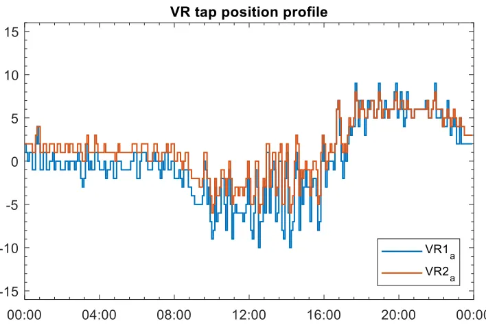
Figure 3.4 LTC and VR tap positions for a heavy load day ... 61

Figure 3.5 Operation sequence of VVC devices in a heavy load day ... 61

Figure 3.8 Apparent power at Inverter 840 A in a heavy load day ... 63

Figure 3.9 Power loss profile in a heavy load day ... 64

Figure 3.10 VR tap operation profile under conventional VVC ... 65

Figure 3.11 Comparison of LTC tap position profile in a heavy load day ... 66

Figure 3.12 Comparison of VR phase A tap position profile in a heavy load day ... 66

Figure 3.13 Comparison of power loss profile in a heavy load day ... 67

Figure 3.14 Comparison between expected power loss and actual power loss ... 68

Figure 3.15 Boxplot of absolute error of expected power loss in VVC ... 68

Figure 3.16 PV and load profile in a light load day ... 69

Figure 3.17 LTC and VR tap positions in for light load day ... 70

Figure 3.18 Operation sequence of VVC devices ... 70

Figure 3.19 Vmax and Vmin profile in a light load day ... 71

Figure 3.20 Power loss profile in a light load day ... 72

Figure 3.21 VR tap operation profile under conventional VVC ... 72

Figure 3.22 Reactive power at Inverter 840 A in a light load day ... 73

Figure 3.23 Apparent power at Inverter 840A in a light load day ... 73

Figure 3.24 Simple diagram of the IEEE 123 Test System [35] ... 74

Figure 3.25 Normalized load and PV profile in a heavy load day ... 76

Figure 3.26 VR4 Tap positions for a heavy load day ... 76

Figure 3.27 Operation sequence of VVC devices in a heavy load day ... 77

Figure 3.28 Vmax and Vmin profile in a heavy load day ... 77

Figure 3.30 Apparent power at Inverter 76 A in a heavy load day ... 79

Figure 3.31 Power loss profile in a heavy load day ... 80

Figure 3.32 Comparison of VR phase A tap position profile in a heavy load day ... 80

Figure 3.33 Comparison of voltage variance in a heavy load day ... 81

Figure 3.34 Voltage statistics in voltage optimization ... 82

Figure 3.35 Power loss of gradient based Var Optimization ... 84

Figure 3.36 Phase A feeder voltage after Var Optimization ... 85

Figure 3.37 Qinj on modified IEEE 123 node system after Var Optimization ... 85

Figure 3.38 Normalized load and PV profile in a light load day ... 86

Figure 3.39 VR4 Tap positions for a light load day ... 87

Figure 3.40 Vmax and Vmin profile in a light load day ... 87

Figure 3.41 Reactive power at Inverter 76 A in a light load day ... 88

Figure 3.42 Apparent power at Inverter 76 A in a light load day ... 88

Figure 3.43 Power loss profile in a light load day ... 89

Figure 3.44 Comparison of VR4 Tap positions in a light load day ... 90

Figure 3.45 Comparison of voltage variance in a light load day ... 90

Figure 4.1 Step voltage change and power response of simple recovery model... 95

Figure 4.2 VVC architecture in system with partial SST deployment ... 101

Figure 4.3 Actual real power measurement of a single-family home ... 102

Figure 4.4 Zoom-in view of power measurement of a single-family home ... 102

Figure 4.7 Voltage measurement at transformer in a winter day ... 106

Figure 4.8 Estimated load parameter in a winter day ... 107

Figure 4.9 Estimation error of recursive estimator... 108

Figure 4.10 Power measurement in selected interval in a winter day ... 108

Figure 4.11 Estimated parameter in selected interval in a winter day ... 109

Figure 4.12 Estimation error in selected interval in a winter day ... 109

Figure 4.13 Comparison of estimated power of load in a winter day ... 111

Figure 4.14 Histograms of error of LS method and Recursive method ... 111

Figure 4.15 Power measurement at transformer in a summer day ... 112

Figure 4.16 Voltage measurement at transformer in a summer day ... 112

Figure 4.17 Estimated load parameter in a summer day ... 113

Figure 4.18 Estimation error of recursive estimator ... 114

Figure 4.19 Comparison of estimated power of load in a summer day ... 115

Figure 4.20 Histograms of error of LS method and Recursive method ... 115

Figure 4.21 Error% of estimated power of load for no-CVR case ... 117

Figure 4.22 Zoomed-in box plot of Error% ... 117

Figure 4.23 Difference between measured of no-CVR case and CVR case ... 118

Figure 4.24 Estimation error of power of load for no-CVR case ... 119

Figure 4.25 Power measurement of CVR case and No CVR case ... 119

Figure 4.26 Estimation error of recursive estimator in selected time interval ... 120

Figure 5.1 A generic architecture of a centralized DMS ... 122

Figure 5.3 Architecture of proposed VVO ... 125

Figure 5.4 DGI architecture... 129

Figure 5.5 FREEDM HIL System ... 130

Figure 5.6 Hardware system of HIL Testbed [58] ... 131

Figure 5.7 Results of VVO implementation on FREEDM HIL Testbed ... 132

Figure 5.8 Hardware system of GEH Testbed ... 133

CHAPTER 1. Introduction

Volt/Var Control (VVC) is the process of managing voltage levels and reactive power (Var) to make the power distribution system work at a desirable operating point. Utilities have been using VVC for many years to maintain acceptable voltages for distribution systems. With the advancement of device technology and analysis methods in power

systems, more advanced VVC, named Volt/Var Optimization (VVO), is under development. In this chapter, the motivations, control devices, benefits and challenges of VVO is

discussed, and a formulation of VVO problem for a smart distribution system is also presented.

1.1 Overview of Volt/Var Control

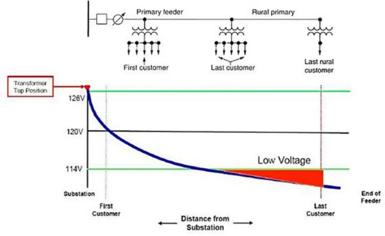
For a distribution system with a radial structure, the voltage drops gradually as the distance from the substation increases. The ANSI C84.1 standard [1] specifies the

recommended “service voltage” for “range A” as ±5% of the nominal value (i.e., 114 V ─ 126 V for a nominal service voltage of 120 V). Under heavy load conditions, without VVC, a distribution system may experience under-voltage violation as shown by the blue line on Figure 1.1. Since distribution system voltage regulation is a fundamental requirement for all utilities, the primary goal of VVC is to maintain the voltages along a distribution feeder within an appropriate range under all operating conditions.

The means to achieve VVC falls into the two following categories: 1) Voltage regulation by LTC or VR

Figure 1.1 Feeder voltage under heavy load condition

In conventional distribution systems, voltage regulators (VRs), load tap changers (LTCs) and capacitor banks (CAPs) are the devices that have been used for Volt/Var control (VVC) purpose. With the increasing penetration level of distributed renewable energy resources (DRERs) on distribution system, PV with smart inverters or solid state transformers (SSTs) are considered as Var control devices [2]. In traditional VVC, VRs and LTCs are controlled based on local measurements, and they are coordinated by differentiating the time-delay setting [3], [4]. In this local control mode, the user can configure the voltage set point of a VR or LTC, and then the controller gives command of increasing/decreasing the tap position to regulate the voltage to the set point by changing the turns ratio. The control of The

current-With the extension of supervisory control and data acquisition (SCADA) to distribution system, the traditional VVC can be improved to achieve more benefits while keeping the voltages acceptable. More advanced controllers with remote control function enable VR, LTC and Caps to receive command by the SCADA system. In remote control mode, VR and LTC receive command of tap increasing/decreasing from the control center [5], [6], and Cap receive command of on/off. On the other hand, high level of DRER penetration imposes new challenges on traditional VVC. Therefore, researchers started to develop more advanced VVC schemes, Volt/Var optimization (VVO), which is a process of optimally managing voltage levels and reactive power to achieve more efficient gird operation by solving an optimization problem.

Although the primary goal of VVO is to keep voltages within acceptable range, the benefit of VVO falls into the following three aspects:

1) Power quality, such as the improvement of voltage profile and power factor. 2) Energy saving, for example power loss reduction and peak demand reduction. 3) Reduction of control cost.

Among the proposed approaches, [7] uses power loss, and [8] uses control cost

minimization as the objective function. Other objectives including demand reduction and power factor correction are mentioned in [9] .

With the promotion of smart grid technology, the planning and operation of distribution systems evolves and VVO should take the challenges associated with the smart features in distribution systems. A traditional distribution system considers discrete control variables (LTC, VR and CAPs) only: LTC and VR change the voltage by moving the taps, and Caps change the reactive power flow by connecting/disconnecting to the feeder. However, in modern distribution system, with the proliferation of DRERs, smart inverters and SSTs reactive power can be injected into the system in continuous amount. Therefore, VVO should be able to handle both continuous and discrete variables. Besides, DRER generation adds more uncertainty to the system net load profile. Traditional VVC runs in an offline manner due to the unavailability of data from real-time monitoring. Even though, with short-term forecasting technology the PV prediction can be updated as frequently as 15 min [15], the actual PV generation may vary in much smaller time interval. In smart distribution system, the SCADA system has the access to real-time data from smart meters at the loads, inverters and/or SSTs at the DRERs, enabling VVO to run in real-time to optimize the system

operation timely. However, for a large distribution with many DRERs and loads, a

centralized VVO scheme has a high communication requirement due to the large number of real-time data exchanged at the control center. This drives the centralized VVO structure into decentralized VVO structure. To address the issues mentioned above a master-slave based master-slave based decentralized VVO architecture is proposed in Chapter 2.

application from Eaton, as shown in Figure 1.2, as an example, IVVC application utilizes the real-time data from LTC, VR, CAPs and monitoring points such as customer meter and medium voltage sensor to find the optimal operation of VVC devices to minimize the operational cost [16]. In centralized IVVC, each device with communication capability exchanges real-time data directly with the RTU (Remote Terminal Unit, a component of SCADA). And the real-time data collected by the RTUs at different substations and remote locations on the feeder are pooled by the MTU (Master Terminal Unit, a component of SCADA) at control center [17]. In some of the available products, the IVVC function will run periodically at a user adjustable time interval (typically ≥ 15 min), or when a significant change in feeder loading occurs.

Figure 1.2 Yukon IVVC Application from Eaton [16]

optimal power flow problem. To formulate the Volt/Var control as an optimization problem, one needs to determine the objective and then the constraints.

The objective of VVO would be minimizing one or a weighted combination of the following terms:

1) Power loss or energy loss [7] 2) Control cost [13]

3) Voltage variation [18] 4) Peak demand [19]

The constraints of VVO include both equalities and inequalities. The equality constraints represent power flow of the system. Due to the high R/X ratio of distribution networks, the non-linear and non-convex power flow equations is not recommended to be simplified into linear form, which makes it challenging to solve the VVO problem. The inequality

constraints include, but are not limited to: 1) Voltage limits

2) Tap position limits of LTC and VR 3) Maximum number of switches for CAPs 4) Line current limits

5) Power factor limit at either substation or other points in the system 6) Three-phase balancing constraints on the main feeder

Based on different selected objective functions and constraints, the VVO problem can be generally classified into the following categories:

2) Mixed Integer Linear Programing problem (MILP), where both the objective function and the constraints are linear, but the variables include both continuous and discrete variables.

3) Non-linear Programing problem (NLP), where either the objective function selected is non-linear or the constraints has non-linear term, and the variables are all continuous variables.

4) Mixed Integer Non-linear Programing (MINLP) problems, where either the objective function selected is non-linear or the constraints has non-linear term, and the variables include both continuous and discrete variables.

The above four types of VVO problem can be solved centrally by directly applying various optimization techniques[20], [21]. An LP VVO can be solved by either simplex method or interior point method, however it applies to a distribution system with continuous control variables only. [10] models the VVO as an MILP problem. Although the accuracy of the MILP model is adequate, the computation time is too long for real-time implementation. In [10], it takes 200-400 s to solve and MILP VVO for a system with 34 nodes. For an NLP VVO, successive linear programing can be used to find the optimal solution. Like the LP approach, this method cannot handle the VVC device operating in a discrete manner, such as Caps and VR. The MINLP VVO is the most difficult one to be solved. [22] uses the mixed integer conic programming technique to solve an MINLP VVO, however it also suffers long computation time, thus not suitable for real-time implementation.

optimization [22], [23]. However, little research has been done to integrate the decentralized optimization based VVO into the DMS system.

1.2 Proposed Volt/Var Control Schemes

In this work, the Volt/Var Control problem is formulated as an optimization problem aiming at minimizing power loss with operating constraints considered.

In conventional distribution systems, voltage regulators, and load tap changers (LTCs) and capacitor banks (CAPs) are the devices that have been used for Volt/Var control (VVC) purpose. With the increasing penetration of DRERs, smart inverters are encouraged to be used as Var control devices [25], [26]. The main contribution of this work is to propose effective Volt/Var Control schemes which utilize both conventional VVC devices and DRER, especially PV systems.

A general formulation of VVO problem to minimize power loss is shown in formulas (1-1) to (1-4).

 

( , ) _loss

min f x u P x (1-1) s.t. g x u( , )0 (1-2)

min max

V  V V (1-3)

min max

u u

u   (1-4)

wherex[ ; V]is the state variable which is the vector containing voltage angles and magnitudes, and u are the control variables which will be discussed in detail later. The full expression of power loss function is in the following equation [27]:





2 2

( , ) g 2 Vcos ,

where gij is the branch conductance, is the set that contains all the nodes in the system. The equality constraints in (1-2) correspond to power flow equations [27]:

 









cos s

, 0 ,

sin s

i

co n

G i Li i j ij ij

inj i i j ij ij ij ij

j

ij ij j

g x u i j

Q V

P P V G

V G B

V B                        





where P_{G i}is the real power generation from the PV at node i, P_{L i}is the real power

consumption at node i, Qinj iis the reactive power injection at node i, i j   i jis the

voltage angle difference between node i and node j, G_{i j} jB_{i j} Y_{i j}is the element of Y-bus matrix.

This work focuses on developing an effective Volt/Var Control scheme for smart

distribution systems with DRERs, especially PV systems. PV systems generating DC power need inverters or SSTs to connect to the grid. These devices have the capability to act as a reactive power sources or sink. Therefore, the dispatchable Var from DRER will be considered as one of the control variables to realize the goal of VVC.

The VVO for smart distribution systems aims at minimizing power loss while keeping feeder voltages acceptable under all operating conditions. The FREEDM Notional Feeder, as shown in the dashed box in Figure 1.3, is used to illustrate how the VVO problem is

within acceptable range. Therefore, on this test feeder there is no need to install VR, LTC or Cap. The objective of the VVO problem on the FREEDM Notional Feeder system is to minimize the power loss as shown by equation(1-5). The voltage magnitude on the feeder is restricted by the constraint in (1-3). Constraint (1-4) indicates that the reactive power from SST should be limited by the capacity of SST. The solution u* of the VVO problem represented in (1-1) – (1-4) is the optimal reactive power injection *

inj

Q of the nine SSTs on FREEDM Notional Feeder.

In a large FREEDM system, for example the FREEDM IEEE 34 System, both voltage regulating devices (LTC and/or VR) and SSTs are using as VVC devices. The solution of VVO u* should give the optimal tap position of each voltage regulating device and the optimal reactive power injection of each SST. The inequality constraint in (1-4) should be expanded into the following inequalities.

inj

min max

Q Q Q (1-7)

min max

LTC LTC LTC

Tap Tap Tap (1-8)

min max

VR VR VR

Tap Tap Tap (1-9)

where Q_injis continuous variable, Tap_LTC and Tap_VR are discrete variables representing the tap positions of LTC and VR. (1-7) indicates that the reactive power injection should be limited by the reactive power capacity of SSTs. The tap position limitations of LTC and VR are represented by the inequalities in (1-8) and (1-9) .

Hence, to be general, the VVO problem for FREEDM System is a non-linear optimization problem with both discrete and continous variables. The discrete variables correspond to voltage control devices, LTC and VR. The continous variables correspond to Var control devices, SST. The solution of the VVO problems should the give the optimal setting of all VVC devices. In reality, LTC and VR are remotely controlled by command of tap

LTC. The SST in the FREEDM system has a local controller to process the command, Q_inj*, therefore no conversion is needed.

In order to solve the optimization problem above efficiently, a two-phase method is proposed in Chapter 2.

1) Phase I: Voltage Problem 2) Phase II: Var Problem

By decompsing a MINLP problem into an integer problem and an NLP problem, the proposed two-phase method is comuputationally efficient to be implemented in real-time VVO. The proposed method can be applied to a master-slave based decentralized control scheme to realized power loss minimization and acceptable feeder voltage. Details of this VVC scheme can be found in Chapter 2.

Chapter 2. Two-phase Volt/Var Control Scheme

Since the IVVC designed for smart distribution systems should be able to react to load and DRER generation change in real-time, a Mixed-Integer Programing solver is not

recommended to be used due to long runtime when discrete variables involved. In this

chapter, a two-phase decoupled VVO method is proposed and implemented as a master-slave based VVC architecture. The effectiveness of the proposed VVC scheme is verified by case studies on two FREEDM Systems, FREEDM Notional Feeder and FREEDM IEEE 34 System.

2.1 A Two-phase VVO Method

Based on the linear model of VR in [7], the power loss change due to VR depends on voltage magenitude change only [7]. Pratically, VR in the system keeps the voltages on the feeder within a tight limits, therefore within the small voltage range power loss change due to VR is small. With voltages regulated in a small, the power loss change is mainly due to CAP’s Var support. Hence, a VVO problem presented in section 1.3 can be decoupled into two problems, Voltage problem (to adjust VR to limit the voltage to a tight range) and Var problem ( to change the Var compensation to minimize the power loss [7]. Since a well-regulated voltage profile is required for decoupling the original VVO, Voltage problem needs to run before solving the Var problem. Figure 2.1 shows a diagram of the two phased

Figure 2.1 Decoupled Volt/Var Optimization Phase I Voltage Problem

combinations are visited in the search, can be adopted to search for the possible tap position combinations of LTC and VRs.

LTC or VR usually has usually 33 taps, including the zero-tap position, and each tap corresponds to a 0.00625 p.u. of turns ratio change. The LTCs are typically three-phase controlled and installed at the substations. In this work, since we use the secondary side voltage of LTC as the slack bus to solve the power flow, the secondary side voltage of LTC can be represented by a set of discrete voltage values in p.u., which indicates the tap position of LTC. Therefore, In the examples and simulation results in this chapter, the tap position of LTC is represented by voltage in p.u.. The tap positions of VR are still represented by integer numbers. For VRs, the three phases are usually controlled independently. For example, a system with one LTC and one VR has possible tap position combinations of 33 × 33 × 33 × 33 = 1,185,921. Therefore, the complete search is not an efficient way to obtain the solution of Phase I problem.

For an operating distribution system, voltages change after the change of system load and/or the output of DG and/or storage devices, therefore VVC devices are expected to make adjustment to follow such changes to achieve feasible voltages. In the proposed two-phase VVO, Phase I brings the system voltages to a small range within 0.95-1.05 p.u. by

time interval is not desired as well. Considering the practical operation of VR and LTC, a complete search on all taps is not necessary.

To avoid such huge number of searches, a searching approach based on [28] is proposed. Instead of searching all possible 33 taps, [28] considers initial tap and two taps up and down for LTC and VR: Tap





smaller number. The proposed search method can narrow down the searching further by applying additional rules to determine Tap.

In this work a backward-forward distribution power flow solver, DPF[29], is utilized to provide power flow solution to evaluate the feasibility of the tap position combinations found. To start the Phase I –Voltage problem, an initial tap position should be given. The search always starts from the substation and moves towards the downstream devices. This is to mimic the time setting to coordinate multiple voltage regulating devices in the system. In the proposed method, the following rules for VR are used to reduce the number of search:

Starting from the voltage control device closest to the substation (e.g. LTC), run DPF for each possible tap position of that device while keeping the taps constant for any other downstream voltage control devices.

1) If no voltage violation occurs, a full search for downstream devices in which





p VR

Tap

    is conducted.

2) If voltage violation occurs, for the downstream devices

i) If 𝑉𝑝𝑚𝑖𝑛< 0.95, TapVRp  





ii) If 𝑉_𝑝𝑚𝑎𝑥 _{> 1.05,} p





Tap

    is conducted, where p represents phase a, b or c, 𝑉_𝑝𝑚𝑎𝑥 _{is the maximum system voltage in phase p.}

The idea of the rules is to avoid searching the increasing taps when over-voltage violation occurs and to avoid searching the decreasing taps when under-voltage violation occurs. Figure 2.2 summarizes the rules above.

Consider the following case as an example:

• Voltage control devices in the system: 1 LTC (three-phase controlled) at substation and 1 feeder VR (single-phase controlled)

• Initial tap positions: Tap_LTC 1.05p.u. and TapVR 





• Initial power flow: 𝑉_𝑏𝑚𝑖𝑛< 0.95 𝑝. 𝑢. and 𝑉_𝑐𝑚𝑖𝑛 < 0.95 𝑝. 𝑢..

• Load condition: heavy load

The first step in the proposed search method is to determine the possible tap position combinations. The next step is to use power flow solver to find the feasible combinations.

In this example, the initial setting of LTC is 1.05 p.u. Since 1.05 p.u. hits the upper voltage limit of the ANSI requirement [1], LTC tap positions higher than 1.05 p.u.

Table 2.1 Possible VR tap positions when LTC tap = 1.05 p.u

∆𝑇𝑎𝑝 -2 -1 0 +1 +2

𝑇𝑎𝑝_𝑉𝑅𝑎 5 6 7 8 9

𝑇𝑎𝑝_𝑉𝑅𝑏 6 7

𝑇𝑎𝑝_𝑉𝑅𝑐 7 8

In the second step, power flow results of all the possible combinations are compared with the voltage upper and lower limits to find the feasible solutions for Phase I problem. Since the solution from Phase I is not unique, a criterion is needed to determine the best solution to initialized Phase II problem. Since Phase II is to minimize the power loss, in order to save the computation effort in Phase II, the tap position combination with least power loss can be selected as the criterion. Solution with the least voltage variance can also be used to initialize Phase II, because power loss with small voltage variance is very close to the minimum power loss.

Phase II Var Problem

tap positions. Therefore, the Var problem only involves continuous and therefore it becomes an NLP optimization problem.

This NLP problem can be solved approximately by a sequential line search method [20], [21] , or Successive Linear Programming (SLP) method. In SLP method, the optimal of an NLP problem is found by solving a sequence of first-order approximations (i.e.

linearizations). In [30] , the Var problem is solved by a SLP method. However, the SLP based method takes much time to update linear model and the determination of linear trust region is challenging for a complicate problem like Var optimization.

In each search along the steepest descent, the gradient f i_u( ) is calculated first (details of calculating f_u is given in Appendix A) and then the control variable is updated as

*

( ) ( 1) ( ) _u( )

u i u i  i f i (2-1)

In each gradient update, the challenge is to determine the best step size *( )i such that the objective function (power loss) is minimized without violating voltage constrains. The best-step size can be found by an inner loop search as shown in Figure 2.4. The power loss shown in Figure 2.3 and Figure 2.4 comes from the power flow solver, DPF, instead of the

summation of objective functions for each phase. As the figure shows, is updated as

(

k

1)

( )

k



 







for some γ > 1. The largest ( )k which achieves the maximum power loss reduction without violating the voltage constraints is selected as*( )i . There’re also other methods

such as Armijo’s rules [21] to determine *

( )i

 . However, to use Armijo’s rules, an effective (neither too large nor too small) (0) should be selected based on Lipschitz constant which is usually unknown for a complicate function like power loss function in VVO [20], [21]. In the proposed method, the initial value (0) is selected such that the minimum change for the

In the proposed method, the gradient is calculated phase by phase, which means problem modeled in equation (1-1) – (1-4) is formulated for each phase. Although, setting total power loss of three phases as the objective and using three-phase power flow equations can be more accurate, the single-phase formulation reduces the dimension of the matrices involved (e.g. Jacobian matrix of power flow equations) in gradient calculation by 2/3.

Start

k=0

Initialization of step-size: β(0) k=0

Initialization of step-size: β(0)

Calculate power loss based on f(i) and β(k)

to get Ploss_old(k)

Calculate power loss based on f(i) and β(k)

to get Ploss_old(k)

β_new(k)= γβ(k) β_new(k)= γβ(k)

Calculate power loss based on f(i) and

β_new(k) to get Ploss_new(k)

Calculate power loss based on f(i) and

β_new(k) to get Ploss_new(k)

Ploss_new(k)<Ploss_old(k)? And there’s no voltage violation Yes k=k+1 k=k+1 No β* =β(k) β(k)=β_new(k-1) Ploss_old(k)=Ploss_new(k-1)

Real-time implementation of VVO involves updating the control every 5-10 minutes. In each control updating period, an 𝑢∗is determined by the proposed VVO method. The

2.2 Master-slave based Volt/Var Control Scheme

In conventional distribution systems, there’s no processing capability at the substation. The VVO problem is solved at the control center managing multiple substations. In centralized VVO scheme, the SCADA system at the control center receives data from all intelligent devices at feeder level. “Centralized” here refers to the topology of the

communication network. Real-time centralized VVO places heavy communication burden on the control center in a system with large number of remote monitoring devices.

Distributed Volt/Var control on smart inverters or SSTs is effective to avoid voltage violation [26], [27]. In this approach, the control is generated locally at the inverter or SST and no centralized communication to the control center is needed. However, such distributed Volt/Var control scheme mainly focus on voltage issue without considering other benefits of VVO, such as power loss reduction. Due to approximations of system models, this approach is lack of system level optimization.

Recent efforts have been made to develop decentralized VVO and there’re several reasons as listed below:

1) Communication requirement is high for centralized VVO scheme 2) The size of a centralized VVO problem can be very large

3) Smart distribution systems enable communication and processing capability at the feeder level

decomposed into smaller sub-problems, have been proposed to solve a large NLP problem. [11] and [14] implement the Dantzig-Wolfe decomposition to decompose the SLP based VVO problem into sub-problems coordinated by the master problem. However, this decomposition technique solves a LP problem at the cost of more iterations to update the master and sub-problems [20] and it has the same drawbacks as the SLP based VVO. Therefore, the proposed two-phase VVO method is computationally more efficient to be considered for real-time implementation for smart distribution systems.

In a smart distribution system, multiple intelligent agents (for example the DGI nodes in FREEDM systems) in the network can compute and communicate. This enables the

implementation of a decentralized control architecture.

Hence, as a trade of between centralized and purely decentralized approach, a master-slave based decentralized VVC architecture is proposed for implementation in smart

distribution systems. In the proposed master-slave VVC architecture, intelligent agents at the feeder level can utilized the real-time data to generate the control for the VVC devices in the system. Therefore, there’s no need to send those real-time data to the control center to utilize the DMS system to run VVO. The proposed master-slave VVC architecture can greatly reduce the data exchange at the control center.

Grouping of the VVC devices

Since a distribution feeder line section can be rather short, the distance between SSTs can be short. And therefore, sensitivity of the power loss to Qinj for the SSTs that are close to

is the case. This observation indicates that we can group the SSTs that are close to each other together and put them under a local “slave controller”, so that all the SSTs in this group can be controlled together. This is the approach used to group the SSTs on a feeder into smaller clusters and develop a decentralized scheme based on this clustering. The grouping results of FREEDM IEEE 34 systems later in section 2.4 can also be verified by applying data mining techniques to power loss sensitivity of each nodes (see in Appendix B).

Master-slave based decentralized VVC architecture

To coordinate the control among the groups, a “master controller” is used to act as a supervisory controller feeding the updated signals to slave units based on the gradient method. In the master, the two-phase approach can solve the VVO problem more efficiently than using MINLP optimization techniques, which enables the proposed VVO to run in real-time. After the solution in Phase II is obtained by the gradient method, the solution vector u* is partitioned according the grouping of SSTs, and then sended to the corresponding slave units, as shown in Figure 2.5. Figure 2.6 shows the participation. The index mi refers to index of VVO slaves, and umi* corresponds to all SSTs managed by slave mi.

After receiving the message for the gradient, each slave allocates the reactive power injection based on the capacity of reactive power support of SSTs. For each SST under a VVO slave, max max * max max 1 1 i i

i i i

i i i Q u u Q     _{ }

Where i max is the total number of SSTs under the slave, i is the index of SST and Qimaxis

the reactive power capacity of SST i. In real-time VVO, u_iis determined in very control period, for example every 5 minutes.

Figure 2.5 Interaction between master VVO and slave VVO

2.3 FREEDM Notional Feeder Results

As shown in Figure 1.3, there is no voltage regulator or shunt capacitor on FREEDM Notional Feeder system. Therefore, without any voltage regulating devices, the VVO

problem becomes an NLP problem, and Phase I is skipped since the SSTs regulate the system voltages well. An SLP based centralized VVO is also simulated to be compared with the proposed decentralized VVO scheme.

2.3.1 Initial System Operating Condition

As mentioned in the previous chapter, SST can automatically work at a unity power factor. Therefore, in the initialization of the algorithm, we set Q_inj 0 , which means the SSTs provide the reactive power demanded by the loads. The loads in the system are set to their peak load values. The substation voltage is assumed to be 1.0 p.u.. Feeders in the

FREEDM Notional Feeder systems, are all three-phase and loads are three-phase unbalanced. Figure 2.7 shows the feeder voltage in phase A at the original system operating condition.

The lowest voltage in phase A in the system occurs at feeder end Node 9. The power flow results of this feeder show that voltages on the primary side are between 1.0052 p.u. and 0.9603 p.u. Therefore, there is no voltage issue on this feeder. The voltages form Node 0 to Node 4 is not monotonically decreasing because of the unbalance of the loads and the coupling effect of three-phase feeder lines. The power loss can be calculated from the power flow results by subtract the total loads from the power at the substation. Under the initial condition above, system has a power loss of 126.7053kW.

2.3.2 VVO Simulation Results on the FREEDM Notional Feeder

Based on the sensitivity test results, the nine SSTs in the system are divided into three groups, shown in Figure 2.8.

Since there’s no voltage control devices in this system, and the voltage profile under the initial condition is satisfactory, we will skip Phase I and go directly to Phase II.

For simplicity, the “updated gradient approach” refers to the sequential line search based on steepest descent. The initial step-size to search for β* in each line search is selected such that the minimum change for the control (SSTs) min

u

 is 0.1 kVar. The detailed convergence information is shown in Table 2.2. The initial system power loss is 126.705 kW. After the first line search along the steepest descent, the power loss is reduced to 122.789 kW. The optimal step-size for the first line search is obtained after 29 inner loop iterations. From the results in the table, the first line search has a power loss reduction of about 4 kW, which is significantly larger than the power loss reduction in other line searches. This verifies the fact that the performance of gradient method gets worse when getting close to the optimal point [20]. The “NA” in the last row of the table means that in the last line search the power loss cannot be further reduced by a small change of control based on initial step-size (0). It takes four sequential line searches (i.e. gradient is updated four times) to converge to the optimal solution. Figure 2.9 shows that the power loss decreases as the gradient is updated, and a total power loss reduction of 4.99 kW is achieved after convergence. Figure 2.10 shows that the minimum voltage is always greater the 0.95 p.u., meanwhile the maximum voltage is always 1.05 p.u.. This indicates the voltages are kept feasible during the Var optimization process. Figure 2.11 shows the path of the reactive power injection of SST4 phase A to reach the optimal.

121.711 kW which is very close to the optimal power loss 121.704 kW calculated by the VVO master. The minimum voltage after decentralized control is 0.977 p.u. From Figure 2.12, we can observe a slight voltage rise within the feasible range in [1] due to the decentralized gradient based VVO.

Table 2.2 Convergence information of the gradient based decentralized VVO

Figure 2.9 Power loss during the gradient based decentralized VVO Iteration for gradient

updating

Power loss (kW)

Vmin (p.u.)

Iteration for step-size search

0 126.7053435 0.960272 29

1 122.7890484 0.977779 24

2 122.5769644 0.976918 25

3 121.7705037 0.979355 21

Figure 2.10 System minimum voltage during the gradient based decentralized VVO

Figure 2.12 Primary feeder voltage on FREEDM Notional Feeder

Figure 2.13 Load level tested on FREEDM Notional Feeder

2.4 FREEDM IEEE 34 Test System Result

IEEE 34 node test feeder is an actual feeder with a nominal voltage of 24.9 kV, as shown in Figure 2.15. It is characterized by its long line length and heavy peak load. An in-line distribution transformer, between node 832 and 888, steps down the voltage to 4.16 kV for a short section of the feeder. Besides, there are two VRs connected between node 814-850 and node 852-832, and two capacitor banks connected at node 844 and 848 separately [32]. These Var compensation and voltage regulation devices are needed to maintain a good voltage profile under all operating conditions. The voltage regulators have 16 tap position range with 10% of maximum voltage change. And the three phases of the VRs are controlled separately. The original IEEE 34 system does not have any DRER.

Figure 2.15 Simple diagram of the original IEEE 34 Test System [32]

FREEDM IEEE 34 system and it is put in the same place as VR1 in the original system. The LTC is assumed to have the same tap range and ratio range as the VRs. However, since the feeder voltage should be between 0.95 p.u. and 1.05 p.u. [1], only taps with voltage in this range is feasible for the LTC. All shunt capacitors are removed as well, since SSTs can provide sufficient reactive power for the purpose of VVC. Figure 2.16 shows the diagram of FREEDM IEEE 34 test system.

Figure 2.16 Simple diagram of FREEDM IEEE 34 Test System

point for peak load condition is simulated. A 24-h simulation is also performed to verify that the proposed method is suitable for real-time implementation. Since results in section 2.3 show that the first line search can provide a solution very close to the optimal, in the following case studies the sequential line search method simplified into single line search along the steepest descent.

2.4.1 Initial System Operating Condition

2.4.2 VVO Simulation Results on FREEDM IEEE 34 Test System

Phase I – Voltage Problem

The number of the possible LTC and VR tap combinations is 3 5 5 5 375    using the method in [28]. By applying the reduced search approach proposed in section 2.1, the number of possible combinations is 168. Since the feasible tap position combination is not unique, Phase II - Voltage Problem returns a list of all feasible tap position combinations. Since the DPF runs for every possible tap position combination, the power loss which comes from DPF results for all feasible combination is also available. It may happen that the

reducing search method proposed finds less number of feasible tap position combinations than the original method in [28]. Thus, the proposed method has the potential to miss the feasible combination with the least power loss, which means a global optimal is not guaranteed. However, it should always finds a solution good enough to initialized the Var Optimization as long as the system is well-designed.

Table 2.3 shows the results of Phase I of the two searching methods, method in [28] and the proposed reducing search method. The results show that the proposed searching method is able to find all feasible combinations and has more than 50% runtime improvement. The runtime results is abtained by running the two methods on the same PC (Intel® Core™ i7-6600U CPU @2.60GHz 2.81GHz, RAM 16.0 GB, 64-bit OS). Since the searching method gives a list of feasible combinations, some criteria are needed to determine which

combination is the one to intialized the Var Optimizaiton process. In this case, the

magnitude) or the metrics proposed in [33]. Results show that the two searching methods give the same feasible solutions.

Table 2.3 Phase I results on FREEDM IEEE 34 System Original Method in

[28]

Proposed method

Number of possible solutions 375 168

Number of feasible solutions 64 64

Best solution found VR=[8 8 8]

and LTC = 1.05 p.u.

VR=[8 8 8] and LTC = 1.05

p.u. Power loss associated with the best

solution (kW)

211.742 211.742

Runtime (s) 4.479 2.021

Phase II – Var Optimization

The updated gradient approach is not adopted to the Var problem on this feeder for the ease of implementation, since the first iteration of the updated gradient approach gives a much more significant power loss reduction compared with the next few iterations. The initial step-size to search for β* is selected such that the minimum change for the control (SSTs) min

u

 is 0.02 kVar. Figure 2.20 shows power loss for the optimal step-size search. As the figure shows, the power loss decreases gradually until it reaches the 16th iteration. After the 16th iteration, power loss starts to increase. And a total power loss reduction of 1.665 kW is achieved at the 16th iteration. Figure 2.21 shows the reactive power injection at Node 840 Phase A of each iteration. As Figure 2.20 and Figure 2.21show, after 16th iteration,

increasing the Var support won’t further reduce the power loss, which means the step-size search stops at the 16th iteration. The minimum voltage before Var Optimization runs is 0.9654 p.u.; after convergence the minimum voltage is 0.9721 p.u.. Figure 2.22 shows the reactive power injection of all phase A SSTs after convergence. The voltage profile before and after VVO is shown in Figure 2.23. As the figure shows, the VVO helps also raise the voltage profile.

Runtime of the proposed VVO for the above case is 0.97s and considerably less than the 3.38s runtime of the SLP based VVO (same PC). This is not only because the gradient based approach has less iterations, but also because each iteration of SLP VVO takes more time to update and solve the LP problem.

Table 2.4 Convergence information of Phase II optimization for FREEDM IEEE 34 System

Iterations Vmin (p.u.)

Vmax (p.u.)

Loss (kW)

Loss Reduction(kW)

Before Phase II 0.965 1.05 211.742

Gradient Method

16 0.972 1.05 210.077 1.665

SLP Method 21 0.973 1.05 209.992 1.750

Figure 2.20 Power loss of gradient based decentralized VVO

Figure 2.22 Reactive power injection at Phase A SSTs

VVO results of a 24-hour simulation

To simulate the operation of the test feeder on a typical day, a 24-hour PV and load profile with a 5-min resolution, shown in Figure 2.24, is used. The goal of this simulation is to test the effectiveness of the proposed VVO in adjusting reactive power injection of SST as the system net load changes.

Figure 2.24 PV and load profile in 24 h

initialize Phase II. In Phase II, the proposed decentralized VVO runs to minimize the power loss and provide additional voltage boost/buck if needed.

In single operating point simulation, the VVO is initialized by a unity power factor at SSTs and certain tap positions of LTC and VR. For a 24-hour simulation, in each control period the VVO is initialized by the present net load condition and the VVC device status returned by the VVO in previous control period. Due to non-convexity of the VVO problem, the line-search method provides solution to a local optimal. For the same peak load condition, in this 24-hour simulation the VVO results is different from the results of the single operating point simulation shown previously, because the same VVO problem is initialized differently.

loss energy is slightly higher than that in the decentralized scheme. Figure 2.28 shows the reactive power injected by SST 840 Phase C at each control period. As the figure confirms, with small load variation at each step, variations of Qinj 840C are small, although the

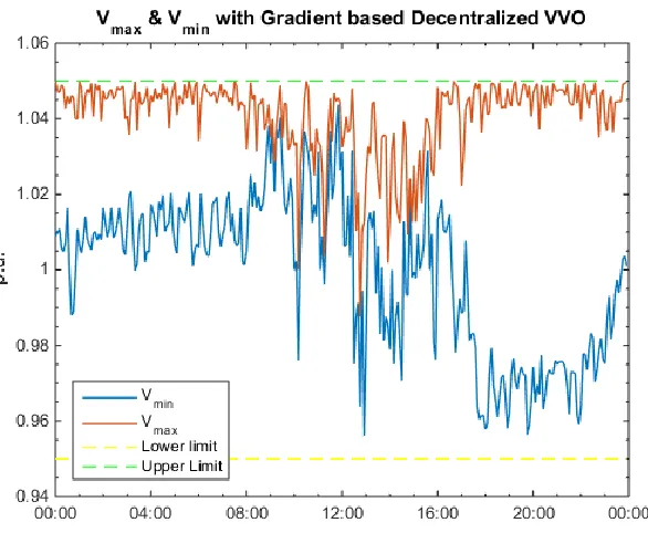
magnitude of Qinj 840C can be considerable especially during the high load conditions. Figure 2.29 shows that the proposed VVC scheme keeps the node voltages within the acceptable range of 0.95-1.05 p.u..

Figure 2.28 Reactive power injection at Phase C SST840 profile

Partial SST deployment

Previous simulations show the test results of systems in which all loads and PV are accommodated by SSTs. However, practically SSTs are installed only at some locations. Therefore, the proposed VVO scheme are test on a modified FREEEDM IEEE 34 system with a few SSTs. In Figure 2.30, locations with SSTs are circled in red. Node 822 has phase A only. Node 844, Node 860, Node 836 and Node 890 have three-phase SSTs.

At peak load condition after Phase I, the system voltage as still within the range of 0.95 p.u. – 1.05 p.u. as shown in Table 2.5. And a total power loss reduction of 10.24 kW is achieved after convergence. Figure 2.31 shows the power loss decreases monotonically and the search stops at the 72nd iteration. The 3-D plots, Figure 2.32 and Figure 2.33 show the initial Qinj and the Qinj after the gradient based method converges. The black line segments on z = 0 plane represents the actual feeder topology. The stems represent the Qinj of at the

locations with loads. After Phase II converges, the Qinj at locations with SSTs become negative, which means SSTs are providing extra reactive power support for the system to minimize power loss.

Table 2.5 Convergence information of Phase II optimization for modified FREEDM IEEE 34 System

Iterations Vmin (p.u.)

Vmax (p.u.)

Loss

(kW) Loss Reduction(kW) Before Phase II 0.957 1.05 221.169

Figure 2.30 Modified FREEDM IEEE 34 Test System

Figure 2.32 Qinj on modified FREEDM IEEE 34 system before Phase II

2.5 Conclusions

In this chapter, a two-phase decentralized Volt/Var optimization scheme is proposed. Two FREEDM test feeders are used to test the proposed scheme. Based on the simulation results, the proposed scheme can effectively reduce power loss while maintaining voltages within feasible region. The two-phase method decouples the MINLP problem into an integer problem and an NLP problem, greatly reducing the computation time. Therefore, the

Chapter 3. Coordinated Volt/Var Control Scheme

Adoption of Photovoltaics (PV) based systems at both residential and commercial scale has accelerated recently. As more PV systems are integrated into a distribution feeder, they will start affecting the voltage control on the feeder, and when the voltage variations become excessive, some mitigation is needed. Conventional Volt/Var control (VVC) devices on the circuit, Load Tap Changer (LTC), Voltage Regulators (VRs), and capacitor banks (Caps), are slow-acting devices. The variability of PV output can also cause excessive operation of traditional VVC devices when PV penetration gets high on the circuit [34], which is also verified by the results shown in previous chapter. This chapter presents a two-level VVC architecture which coordinates the slow-acting devices with the fast-acting devices, providing effective voltage control and mitigating excessive operation of LTC and VRs. 3.1 Two-level coordinated Volt/Var Control

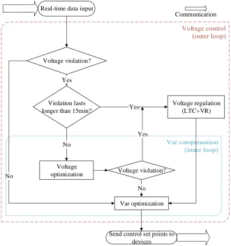
Voltage Control loop – uses LTC and VRs to adjust the voltage level on the circuit to keep the voltages along the circuit within the desired limits. The second level is the reactive power compensation loop which determines reactive power output of inverters needed to smooth the fast voltage variations while providing effective power factor correction to keep the power losses at minimum. Figure 3.1 shows the proposed architecture. The proposed coordinated two-level VVC scheme is computationally efficient, easy for practical implementation, and accommodates the operating constraints.

Real-time data input

Voltage regulation (LTC+VR)

Voltage optimization

Send control set points to devices

Var optimization Violation lasts

longer than 15min? Yes Voltage violation?

Yes

No

No Voltage violation?

No

Communication

Yes

Voltage Control Loop

The voltage control devices, LTC and VRs, are very effective in adjusting the voltage along the feeder, but they are slow acting devices. Hence, the goal in voltage control loop is to monitor the net load variations along the feeder, filter out the fast variations and have the voltage control devices respond only to slow variations. This prevent excessive device operation. This loop is slow, (which is chosen as 15 min in this paper) and provides the supervisory set points for the LTC and VRs. Details of the method adopted for this module has been presented in previous chapter.

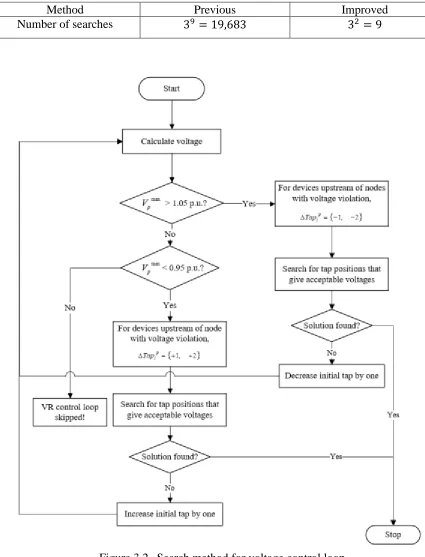
However, the searching increases exponentially as voltage regulation devices increase. In a system with 3 single-phase controlled three-phase VR, ±2 tap range would result in 59 ₌ 1953125 searches, which will increase the computation effort significantly. To resolve this, the topology information of the test feeder is used to reduce the searches.

Practically, the backbone of a feeder has no more than 2 single-phase controlled VRs and other VRs are placed at the beginning of the laterals connected to the backbone, which means there is no more than 2 VR zones from the source of the feeder to one end of the circuit. When a voltage violation is detected, the VVO start to trace voltage regulation device and the phase of taps that are upstream of the nodes of violation. Then only VRs that are upstream of the violation nodes react to the violation with tap changes on respective phases. Figure 3.2 shows this voltage control loop logic.

Table 3.1 Tap search comparison for example case

Method Previous Improved

Number of searches 39 = 19,683 32 = 9

Var Compensation Loop

As indicated above, this module uses an optimization method to determine the proper Var support needed from inverters or SSTs in the system. The objective of Var compensation, under normal conditions, is to improve system efficiency by reducing power loss on the system. However, when there is need for extra Var support to correct voltage violations, the module determines this extra Var support first. In the latter case, the problem formulation is the same as Phase II problem in (1-1) – (1-4), but with a different objective function as shown in (3-1).









( ) 1.0

1

n

f x _i V_i i 

   

 (3-1)

where





0 0.95, 1.05 1 if V i i otherwise i     







3.2 FREEDM IEEE 34 Test System Result

To demonstrate the effectiveness of the proposed VVC scheme in a more practical case, we assume that smart inverters with a lower cost than SSTs accommodate all PV systems on 34 node system. In previous tests, the SST rating is oversized with 25% more than peak load, i.e. 1.25 max

load

N

S  S . In the following case studies, the rating of the smart inverters is

oversized with 25% more than peak generation, i.e. 1.25 max

PV N

S  P . The available reactive power varies as the PV output changes:

2 2

max

( ) _N ( )

PV

Q t  S P t _(3-2)

In this chapter, the proposed coordinated VVC method is tested on two smart distribution systems, 1) FREEDM IEEE 34 Test System with PV systems at all locations, and 2) a modified IEEE 123 System with PV at some locations. The performance of the coordinated VVC method for both a heavy load day and light load day are presented as well.

Voltage Optimization by Var compensation

To test the effectiveness of the gradient based method to determine Var support to resolve voltage violation, a light load condition where voltage violation occurs due to sudden change in PV output (event corresponds to 10:05 am in Figure 2.24) is tested. In this case, LTC and VR do not respond to this event, but the Var support module reacts and determines extra Var support needed from the inverter to eliminate the voltage violation. Here, the updated

gradient method is adopted, because as the indicator variables 𝑤𝑖 changes the gradient vector

of the method. As the figure shows, the node voltages move towards the acceptable ranges quite rapidly and it takes only a few iterations to bring the voltages within 0.95 – 1.05 p.u..

Figure 3.3 Box plot of voltage variation in voltage optimization Case 1: Heavy load day

The goal of this simulation is to test the effectiveness of the proposed VVO in adjusting reactive power injection of smart inverters as the system net load changes in a heavy load day. Figure 2.24 represents a heavy load day which is used to create the PV generation and load profile.

occurs due to sudden change in PV output. These points thus show that indeed Var support helps to respond the sudden voltage violations quickly and this in turn reduces the excessive operation of voltage regulation devices.

Figure 3.4 LTC and VR tap positions for a heavy load day

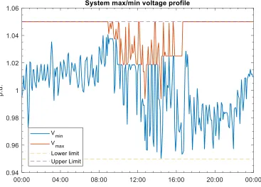
Figure 3.6 Vmax and Vmin profile in a heavy load day

Figure 3.6 confirms that the system maximum and minimum voltages are always kept within the range 0.95 – 1.05 p.u.. In the original IEEE 34 system with conventional control scheme, there’s over voltage violation during the day time with high PV generation [33] and under voltage violation during the time with heavy load[32]. Compared with the

Figure 3.7 Reactive power at Inverter 840 A in a heavy load day

Figure 3.9 shows the power loss profile under both the proposed method and the conventional VVC (used on the IEEE 34 node test feeder) during the day. The results indicate that the proposed VVC provides considerable power loss reduction compared to the conventional VVC scheme: the total energy loss during the day in this case is 36.7% lower than that of the conventional VVC scheme. Figure 3.10 shows the Phase A tap operations of two VRs in the original system. As expected, with variability of system PV output and load, as shown in Figure 2.24, conventional VR control results in excessive tap operations. Compared with Figure 3.4, the proposed coordinated VVC scheme reduces the operation of VR and LTC significantly.

Figure 3.10 VR tap operation profile under conventional VVC

To verify the effectiveness of the proposed voltage control scheme, the 24-h simulation is repeated with a different voltage control scheme. In this case, an exhaustive search method employed for determining the optimal tap settings for voltage control devices when they need to respond to slow load changes. Figure 3.11 and Figure 3.12 show the LTC and VR Phase A tap profiles for the two methods. The two figures show that the exhaustive search method moves the taps more often with finer adjustments, as expected. The main benefits of these adjustments are better loss reduction, as shown in Figure 3.13. However, the cost associated with excessive tap operation may outweigh the additional improvement in power loss reduction.

average, with same PC Tech Spec as simulations in Chapter 2). This clearly indicates the feasibility of the method in practice.

Figure 3.11 Comparison of LTC tap position profile in a heavy load day