Volume 4, No. 9, July-August 2013
International Journal of Advanced Research in Computer Science
RESEARCH PAPER
Available Online at www.ijarcs.info
ISSN No. 0976-5697
HPAARM: Hybrid Parallel Algorithm for Association Rule Mining
Prathyusha Kanakam
Dept. of Computer Science & Engineering University College of Engineering, JNTUK
Vizianagaram, A.P, India. [email protected]
S Radha Krishna
Assistant Professor of CSE University College of Engineering, JNTUK
Vizianagaram, A.P, India [email protected]
Abstract: Data mining is one of the vast areas of research and nowadays the research is going on the most important techniques for decision making processing in data mining. Discovering patterns or frequent episodes in transactions is an important problem in data mining for the purpose of inferring rules from them. So, mining association rules is considered as powerful technique in the data mining process. The problem of mining association rules is composed of finding the large itemsets and to generate the association rules from these itemsets. To find the large itemsets, the dataset must be scanned many times. Many algorithms have been developed to increase the performance of mining association rules through reducing the number of scans over the dataset. In this paper, we aims to enhance and optimize the process even further by developing techniques to reduce the number of database scans to just only once. To deal with the huge size of the data, we have designed a parallel algorithm for reducing both the execution time and the number of scans over the database, in order to minify I/O overheads as much as possible. In this paper, we introduce some approaches for the implementation of two basic algorithms for association rules discovery (namely Apriori and Eclat). Our approach combines efficient data structures (Radix Trees) to code different key information (line indexes, candidates). We also introduced different types of efficient data structures and their merits and de-merits of using them in deducting association rules.
Keywords: Data mining; Patterns, Association Rules; Parallel Algorithm Item Sets; Apriori; Eclat; Radix Trees; Line Indexes;
I. INTRODUCTION
Data mining is an interdisciplinary subfield of computer science, and it is the computational process of discovering patterns in large data sets involving methods at the intersection of artificial intelligence, machine learning, statistics, and database systems. The overall goal of the data mining process is to extract information from a data warehouse and transform it into an understandable structure for further use.
Association Rule Mining (ARM) is one of the most important data mining tasks. Association rule learning is a popular and well researched method for discovering interesting relations between variables in large databases. It is intended to identify strong rules discovered in databases using different measures of interestingness [16]. Association rules are introduced for discovering regularities between products in large-scale transaction data recorded by point-of-sale (POS) systems in supermarkets based on the concept of strong rules [17]. One of the excellent applications of ARM is market-basket analysis [1], here in the market basket analysis the items represent products, and the records represent point-of-sales data at large grocery stores or department stores. For example association rules might be, “90% of customers buying product A also buy product B.” like, 80% people who buy a cot may also buy mattress or who buy a computer may also buy antivirus software. In addition to the above example from market basket analysis association rules are employed today in many application domains including Web usage mining, intrusion detection, Continuous production, bioinformatics, Medical diagnosis and Protein sequences, CRM of credit card business, customer segmentation, catalog design, store layout, and telecommunication alarm prediction [15].
In ARM for ‘m’ items, there are potentially 2m itemsets, whose support is above minimum support. Enumerating all itemsets is thus not realistic. However, for practical cases, only a small fraction of the whole space of itemsets is above a minimum support requiring special attention to reduce memory and I/O overheads. In order to reduce these memory and I/O overheads, we introduced a hybrid parallel algorithm along with efficient data structures (Radix trees) to store the dataset and to perform set operations for the purpose of generating frequent itemsets and association rules by scanning dataset only once.
We organized our paper in 8 sections. In section 1, we introduced ARM. We define our problem statement in section 2. In section 3, we introduce sequential, parallel algorithms and their characteristics, as well as basic sequential and parallel frameworks that are widely used in the literature. In section 4, we introduce different data structures and their merits and de-merits. Radix Tree data structures and their potential use in the process of association rules discovery are described in section 5. We proposed a hybrid parallel algorithm for association rule discovery in order to generate frequent itemsets by combining the features of both APRIORI and ECLAT algorithms by using Radix Trees in section 6. We show some results based on our experimental evaluation in section 7. Finally we conclude our paper in section 6.
II. PROBLEMSTATEMENT
The rule A⇒B has confidence c in the transaction set D, where c is the percentage of transactions in D containing A that also contain B. This is taken to be the conditional probability, P(B∣A).
Rules that satisfy both minimum support threshold (min sup) and a minimum confidence threshold (min conf) are called Strong Association Rules. Association rules are created by analyzing data for frequent patterns and using the criteria support and confidence to identify the most important relationships.
Support is an indication of how frequently the items appear in the database i.e., the occurrence frequency of an itemset is the number of transactions that contain the itemset [1]. This is also known, simply, as the frequency, support count, or count of the itemset.
Confidence indicates the number of times the if/then statements have been found to be true i.e., It is the “trustworthiness” of pattern. It is the measure of certainty associated with validity [1].
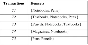
To illustrate the concepts, we use a small example from the Bookshop domain. The set of items is I= {Notebooks, Pens, Pencils, Textbooks, Magazines} and the different transactions in the database are,
Table 1:Data Base of Transactions
Transactions Itemsets
T1 {Notebooks, Pens}
T2 {Textbooks, Notebooks, Pens }
T3 {Pencils, Notebooks, Textbooks}
T4 {Magazines, Notebooks}
T5 {Pens, Pencils}
For the above mentioned data in Table I, let us assume min_sup = 40% (i.e.., support threshold = 2) and min_conf = 80%. Now, we obtain the frequent set = {Pens, Notebooks, Textbooks, Pencils} with sup = 2/5 and we generate the following association rules as,
Pens → Notebooks, Textbooks [sup = 2/5, conf = 4/3] …
…
Pencils → Pens, Notebooks [sup = 2/5, conf = 4/3].
Association rules are useful for analyzing and predicting customer behavior. They play an important part in shopping basket data analysis, product clustering, store layout and catalog design.
III. ASSOCIATIONMININGALGORITHMSANDTHEIR
CHARACTERSTICS
Many algorithms are used for generating association rules and for mining frequent itemsets. Some well known algorithms are Apriori, Eclat and FP Growth.
A. Sequential Algorithms:
Sequential pattern mining finds interesting patterns in sequence of sets. Mining sequential patterns has become an important data mining task with broad applications. For example, supermarkets often collect customer purchase records in sequence databases in which a sequential pattern would indicate a customer’s buying habit.
Sequential pattern mining is commonly defined as finding the complete set of frequent subsequences in a set of sequences. Much research has been done to efficiently find such patterns. But to the best of our knowledge, no research has examined in detail what patterns are actually generated from such a definition. In this paper, we examined the results of the support framework closely to evaluate the frequent patterns.
The design space for the sequential methods is composed of the following characteristics [3][4].
a. Bottom-up Vs. Hybrid search: ARM Algorithms differ in the manner in which they search the itemset lattice spanned by the subset relation. Most approaches use a level-wise or bottom-up search of the lattice to enumerate the frequent itemsets. If long frequent itemsets are expected, a pure top-down approach might be preferred. Some authors proposed a hybrid search, which combines top-down and bottom-up approaches.
b. Complete Vs. Heuristic Candidate Generation: ARM algorithms can differ in the way they generate new candidates. A complete search, the dominant approach, guarantees that we can generate and test all frequent subsets. Here, complete doesn’t mean exhaustive; we can use pruning to eliminate useless branches in the search space. Heuristic generation sacrifices completeness for the sake of speed. At each step, it only examines a limited number of “good” branches. It is also possible to locate the maximal frequent itemsets by using Random Search. Genetic algorithms and simulated annealing are the various methods used for Heuristic generation. Because of a strong emphasis on completeness, ARM literature has not given much attention for these two methods.
c. All Vs. Maximal Frequent Itemset Enumeration: Comparing to all algorithms, ARM algorithms were differ in depending on whether they generate all frequent subsets or only the maximal ones. In ARM algorithms, identifying the maximal itemsets is the core task, because an additional database scan can generate all other subsets. Nevertheless, the majority of algorithms list all frequent itemsets.
Table 2: Horizontal Layout
Transactions Itemsets
T1 I1,I2,I3,I5
T2 I2,I3,I4
T3 I4,I5,I6
Table 3: Vertical Layout
Transactions Itemsets
The sequential ARM algorithms developed are designed to find frequent itemsets and generate association rules. Here, we discuss few of them. These algorithms are classified on the basis of data layout and the data structure [4] used as shown in the following Table IV.
Table 4: Classification of Algorithms
Algorithm Data
Apriori, DHP Horizontal Bottom-up Hash Tree
SEAR,SPEAR,SPINC Horizontal Bottom-up Prefix Tree
Eclat, Clique Vertical Bottom-up None
Partition Vertical Bottom-up None
MaxEclat, MaxClique
Vertical Hybrid None
DIC Horizontal Bottom-up Trie
SPTID Vertical Bottom-up Prefix Tree
e. Apriori Algorithm: In this paper, we explained the basic sequential algorithm: APRIORI. The “Apriori” algorithm forms the core [5] of all parallel [3] association rules discovery algorithms. It uses the principle that a subset of frequent itemset is also frequent, i.e.., frequent k+1 set is generated if and only if there exists frequent k itemsets. This algorithm has three main steps, iterated while new candidates are generated:
Construction of the set of new candidates; Support Evaluation for each new candidates;
Pruning of candidates that have not a sufficient support regarding to a minimum support arbitrarily chosen;
The Apriori algorithm is as follows: Ck:Candidate itemset of size k
Lk: frequent itemset of size k
L1= {frequent items}; for(k= 1; Lk!=∅; k++) do begin
Ck+1= candidates generated from Lk;
for each transaction t in database do increment the count of all candidates in Ck+1 that are contained in t Lk+1= candidates in Ck+1 with min_support;
end
return ∪kLk;
Note that Ck is the Candidate itemset of size k and Lk is the frequent itemset of size k at transaction t ∊ D (data base).
B. Parllel Algorithms:
Researchers expect parallelism to relieve current ARM methods from the sequential bottleneck, providing scalability to massive data sets and improving response time. Achieving
good performance on today’s multiprocessor systems is not trivial. The main challenges include synchronization and communication minimization, workload balancing, finding good data layout and data decomposition, and disk I/O minimization (which are especially important for ARM).
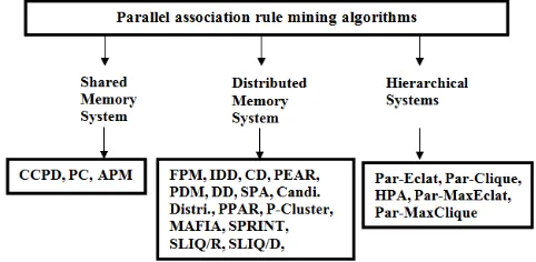
The parallel design space spans three main components: the hardware platform (Fig. 1), the type of parallelism, and the load-balancing strategy [3].
a. Distributed Vs. Shared Memory Systems: Mainly we use two approaches for multiple processors. They are, distributed memory (where each processor has a private memory) and shared memory (where all processors access common memory) [3][4].
A Shared Memory Processor has direct and equal access to all the system’s memory and they used to implement parallel programs on themselves.
Figure 1. List of Parallel association rule mining algorithm developed so far for homogeneous system that uses static load balancing technique on different
machines i.e. shared memory, distributed and hierarchical memory system.
In Distributed-Memory (DMM) architecture, each processor has its own local memory which can access directly. It solves the scalability problem by eliminating the bus, but at the expense of programming simplicity.
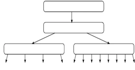
b. Data Vs. Task Parallelism: Task and data parallelism are the two main paradigms for exploiting algorithm parallelism as shown in Fig 2. For ARM, data parallelism corresponds to the case where the database is partitioned among P processors-logically partitioned for SMPs, physically for DMMs.
Task parallelism corresponds to the case where the processors perform different computations independently, such as counting a disjoint set of candidates, but have or need access to the entire database.
Figure 2. Categorization of parallel ARM algorithms on the basis of different Parallelism technique used.
c. Static Vs Dynamic Balancing: Static load balancing initially partitions work among the processors using a heuristic cost function; no subsequent data or computation movement is available to correct load imbalances resulting from ARM algorithms’ dynamic nature. Dynamic load balancing incurs additional costs for work and data movement, and also for the mechanism used to detect whether there is an imbalance. Dynamic load balancing is especially important in multiuser environments with transient loads and in heterogeneous platforms, which have different processor and network speeds.[3][4].
Here, in our paper, we discuss two basic parallel algorithms namely count distribution and Eclat algorithm.
d. Count Distribution: The Count Distribution parallel algorithm is simply a parallel version of Apriori algorithm. Each processor has a copy of the database. It computes "local" candidates and evaluates the "local" supports and transmits them to a dedicated processor to perform the prefix sum of all of them to obtain the global support of the itemset[2].
a) It is required to scan the database for each iteration. Furthermore they enumerate each candidate itemset as many times as we find it in the database even if the transactions are identical.
b) The transaction database is considered to have a horizontal layout.
e. Eclait Algorithm: An advantage of “Eclat” [6] over “Count Distribution” is that it scans the database only two times. Firstly it builds the 2-itemsets and secondly to transform it into a vertical form. Eclat algorithm has three steps.
a) The initialization phase: construction of the global counts for the frequent 2-itemsets.
b) The transformation phase: partitioning of the frequent 2-itemsets and scheduling of partitions over the processors. Vertical transformation of the database. c) The Asynchronous phase: construction of the frequent
k-itemsets. Algorithm for Eclat:
Begin Eclat
/*Initialisation phase*/
Scan local database partition
Compute local counts for all 2-itemsets Construct global L2 count
/*Transformation phase*/
Partition L2 into equivalence classes Schedule L2 over the set of processors P Transform local database into vertical form Transmit relevant tid-lists to other processors
/*Asynchronous Phase*/
for each equivalence class E2 in local L2 ComputeFrequent(E2)
/*Final Reduction Phase*/
Aggregate Results and Output Associations
End Eclat
This algorithm uses an equivalence class partitioning schema of the database. The equivalence class is based on common prefix assuming that itemsets are lexicographically sorted. For instance AB, AC, AD are in the same equivalence SA class because of the common prefix A. Then candidate itemsets can be generated by joining the members of the same equivalence class [2].
We can observe that itemsets produced by an equivalence class are always different of those produced by a different class, then the equivalence partitioning scheme can be used to schedule the work over the processors. This method is used in other algorithms such as Candidate Distribution [2].
The transformation phase is the most expensive step of the algorithm. In fact, the processors have to broadcast the local list corresponding to transaction identifier, for the itemsets to all other processors [2][6].
IV. DIFFERENTDATASTRUCTURESANDTHEIR
MERITS,DE-MERITS
In order to store different transactions, we need data structures to store the data in the database because it is the structure to hold the data. There are different types of data structures available in the literature. Let us discuss a few among them.
A. Balanced Search Trees:
A tree is balanced of each sub-tree is balanced and the height of two sub-trees differ by most one. It is also known as Self-Balancing or Height Balanced binary search tree that automatically keeps its height (maximal number of levels below the root) small in the face of arbitrary item insertion and deletions [8].
The tree is only balanced if
The left and right subtrees heights differ by at most one. The left sub-tree is balanced.
The right sub-tree is balanced.
In the above Un-Balanced tree, node accesses take 3.27 on an average while we traverse from the root to the node. In Balanced tree, node accesses take 3.00 on an average while we traverse from root to the node. So, the path effort decreased in balanced tree.
Most operations on a binary search tree (BST) [8] take time directly proportional to the height of the tree. So it is desirable to keep the height small. A Binary tree with height h can
contain at most nodes. If
follows that for a tree with n nodes and height h.
a. Merits: These structures provide efficient implementation for mutable ordered lists, and can be used for other abstract data structures such as associative arrays, priority queues and sets.
They justified in the long run by ensuring fast executions of later operations.
b. De-Merits: They did not permit lookup, insertion, deletion in O (k) time rather than O(logn). It is not an advantage since normally k log n.
It takes ‘m’ comparisons to look up a string of length ‘m’. But radix tree can perform in fewer comparisons.
B. Prefix Tree:
A Prefix tree is also known as ‘trie’. The term trie comes from retrieval [7] [9]. It is an ordered multi-way tree data structures which is used to store strings over an alphabet. Unlike a binary search tree, no need in the tree stores the key associated with that node; instead its position in the tree shows what key it is associated with. Each node contains an array of pointers, one pointer for each character in the alphabet and all the descendants of a node have a common prefix of the string associated with that node. The root is associated with the empty string and values are normally associated with every node, only with leaves.
A trie is a tree data structure for storing strings or other sequences in a way that allows for a fast look-up. In its simplest form it can be used as a list of keywords or a dictionary. By associating each string with an object it can be used as an alternative to a hash map.
The basic idea behind a trie is that each successive letter is stored as a separate node. To find out if the word 'cat' is in the list you start at the root and look up the 'c' node. Having found the 'c' node you search the list of c's children for an 'a' node, and so on. To differentiate between 'cat' and 'catalog' each word is ended by a special delimiter.
The below Fig. 3 shows a schematic representation of a partial trie:
Figure 3. Schematic representation of a partial trie.
a. Merits:
Look ing up d ata in a trie is faster in worst case. Ο(m)
time(where m is the length of search string) compared to imperfect hash table.
There are no collisions of different keys in a trie.
Buckets in a trie which are analogous to hash table buckets that store key collisions are necessary only if a single key is associated with more than one value.
There is no need to provide a hash function or to change hash functions as more keys are added to a trie.
A trie can provide an alphabetical ordering of the entries by key.
b. De-Merits:
They are slower in some cases than hash tables for looking up data, especially if the data is directly accessed on a hard disk drive or some other secondary storage vice where the random access time is high compared to main memory.
Some keys such as floating point numbers, can lead to long chains and prefixes that are not particularly meaningful.
Some tries require more space than a hash table, as memory may be allocated for each character in the search string.
C. Adaptive Radix Tree
Adaptive Radix Tree is the space efficient and solves the problem of excessive worst case consumption, by adaptively choosing compact and efficient data structures for internal nodes [10] as shown in Fig.6.
ART which is fast and space efficient in-memory indexing structure specifically tuned for modern hardware. ART adapts the representation of every individual node. By adapting each inner node locally, it optimizes the local space utilization and access efficiency at the same time.
Nodes are represented using a small number of efficient and compact data structures, chosen dynamically depending on the number of child nodes. Two additional techniques, path compression and lazy expansion allow ART to efficiently index long keys by collapsing nodes and thereby decreasing the tree height.
Figure 4. Adaptively Sized Nodes
Normally, a tree contains two types of nodes: Internal nodes (or) Inner nodes and Leaf nodes. Unlike other trees (Fig 5.), ART contains special nodes called adaptive nodes [10] along with these nodes as per Fig.4. These nodes are for pure lookup performance, it is desirable to have a large span (determines the height of the tree for a given key length). When arrays of pointers are used to represent inner nodes, usage of space can be excessive when most child pointers are null.
Figure 5. Other Trees with Array Nodes
idea that achieves both space and time efficiency is to adaptively use different node sizes with the same, relatively large span, but with different fan-out. Adaptive nodes do not affect the structure (height) of the tree, only the sizes of the nodes. By reducing space consumption, adaptive nodes allow to use a large span and therefore increase performance too.
Figure 6. ART with Adaptive Node
a. Merits:
It maintains the data in sorted order as hash table.
It performs additional operations like range scan and prefix lookup.
It solves the problem of excessive worst-case consumption. It optimizes the local space utilization and access efficiency at the same time.
b. De-Merits:
Each ART is of variable length.
It is not suitable for comparing two trees which plays a key role in our paper.
It is very difficult to implement these data structures.
D. Radix Tree:
Radix tree plays a crucial role in our paper and we discuss in next section.
V. ACTOFRADIXTREEINASSOCIATIONRULE
MINING
A Radix Tree (also patricia trie or radix trie or compact prefix tree) is a space-optimized trie data structure where each node with only one child is merged with its child [11] . The result is that every internal node has at least two children. Unlike in regular tries, edges can be labeled with sequences of elements as well as single elements. This makes them much more efficient for small sets (especially if the strings are long) and for sets of strings that share long prefixes. As an optimization, edge labels can be stored in constant size by using two pointers to a string (for the first and last elements).
The tree shown below in Fig.7 is of three levels deep. When the kernel goes to look up a specific key, the most significant six bits will be used to find the appropriate slot in the root node. The next six bits then index the slot in the middle node, and the least significant six bits will indicate the slot containing a pointer to the actual value. Nodes which have no children are not present in the tree, so a radix tree can provide efficient storage for sparse trees.
Figure 7. Structure of Radix Tree
Radix Trees [2] are used to store sets of strings over an alphabet. In this paper, the binary alphabet is used because we handle integers representing indexes of transactions.
There are two types of Radix Trees based on the kind of strings we use. If we use Fixed length strings – all strings are of same length for instance 001,011,101,110 here all the example strings of same length 3. In these type of radix trees, all the leaf nodes stores the words (Black nodes indicates that it stores a string) where as variable length strings are of different lengths for instance 0, 10, 110, 111 unlike fixed length strings each are of distinct lengths and the words can be stored in not only leaf nodes but also internal nodes (Black nodes indicates that it stores a string).
Figure 8. Fixed Length Strings
Figure 9. Variable Length Strings
In the above fig. 8 and fig. 9, we represent two types of nodes: black nodes and white nodes. The white color node means that no word is stored in a node. Conversely, a black node means that a word is stored in the node. For instance, if we are looking for word 1 0 in a Radix Tree with variable length strings [2], we follow the right edge (1), then we follow the left edge (0) and we check the color of the node. If the color is white, then the word does not exist in the tree, otherwise the color is black by construction.
In a Radix Tree with fixed length strings [2], we don’t need any color because if a word doesn’t exist then there is no path for it in the tree. It is more convenient for implementing tree management operations efficiently and easily by using these types of structures.
A. Operations on Radix Trees:
Radix Trees represent sets of string in a sorted way. Their tree structure makes the set operations (union, intersection) easier to parallelize. In order to do this, the size of data is constant and known.
paper we perform intersect operation between two Radix Trees to discover association rules as shown in the below fig. 10.
Figure 10. Intersection of Two Radix Trees
For instance for the intersect operation [2], we consider the two roots of two trees to be intersected. If they have two left children in common, then we add a left child to the new tree and we start a new pointer in order to build the “left part” of the intersection. The same procedure is followed for right child and its part.
B. Storing the data using Radix Trees:
In practical applications, we have to deal with huge quantity of data so we need methods to store that large data on disk. In “A hierarchical database management algorithm”, a method has been introduced and implemented successfully to store that large amount of data[12]. This method represents the Radix Tree by bit vectors stored on disk. This solution implements Radix Trees on disk is to store them on an organization with multiple files.
A file organization is adapted which consists some files contained in a directory in order to avoid expensive file system operations. Too large files cause poor response time for updates in the same way too mini files in the same directory could slowdown the application. So, we use a directory structure containing small files which are quickly updateable. In [12], the items of the database are indexed by storing their identifier in a Radix Tree stored in a directory tree structure, in which each directory contains three files.
A file to store the thesaurus (database item lexicon) of the items and the offset of their bit vector on the second file (1).
A file to store the bit vectors of the identifiers for level n (2).
A file to store a permutation of the words giving the lexicographical order (3).
In order to search the lines where an item appears, we consult the permutation file (file 3). This gives the position the word in the thesaurus (file 1) where we can read its bit vector offset in the file (file2).
The representation of integer set with Radix Trees allows us to save space and to implement efficient searches. Indeed, the common prefixes of different integers are stored only once. The computation of key for efficient parallel implementations of tree management operations (union, intersection) can be achieved concurrently on each node at same level in the Radix Tree. We also use Radix Trees in the context of association rules discover, for candidate generation.
C. Representation of item:
Radix Trees are used to code the line indexes of each item in a database [12]. For instance, Consider student table (Table V) which contains the student details contains columns
student_id, student_name, date of admission, course_name
each of them is treated separately: for each of these columns, one builds its thesaurus and for each word of the thesaurus we build the set of line indexes it occurs at.
Table 5. Student Details Table
From the above Table V, we generate association rule as
Course_name = MCA and Student_id = 1004. For
Course_name, it will generate {1,2} and for Student_id {2} appears. So, the frequent item which satisfies this association rule is {2}.
The intersection can be implemented efficiently because we use the number of bits in the representation of integers (in fact we use fixed size alphabet) and not the number of items in the two sets.
The candidate’s k-itemsets are then represented in the same way. For example, if the path in the Radix Tree to the item A is 00 and the path to B is 01, then the path to AB will be 0001.
D. Generation of itemset:
The new candidates for association rules discovery can be generated by joining the members of a same equivalence classes the radix tree is same as prefix tree [2]. It is clearly explained in [2][7][9] respectively.
In order to generate next candidate sets, we have to join the members of the equivalence classes. According to join operation, Radix Tree implementation of the itemsets consists in rooting the initial subtree on each leaf, considering only leaves obtained by following the left neighbors to the current itemset.
For instance, consider the following Fig.11. To obtain the ABC candidate, we join AB and AC with a Radix Tree rooting operation. To get all the candidate sets, we just have to proceed the rooting of subtrees (with the elimination of left nodes) on each leaf. In our case ABC = AB ∪ AC, ABD = AB
∪ AD, ACD = AC ∪ AD.
Figure 11. Candidate Representation
Moreover, by performing the intersection of the identifier trees in parallel we obtain the support of the new candidate. As with the Count Distribution Algorithm, we only broadcast local supports to evaluate the global support.
Student_ id Student_ name Date_Of_ Admission
Course_ name
Index_no
1000 Sampath 02-jun-07 MCA 1
1004 Raju 07-may-07 MCA 2
1007 Jothsna 09-jun-09 MSc 4
Before obtaining the different supports of a candidate set we can eliminate the candidates from the local tree that don’t appear in the local database (i.e supports = 0). If AB doesn’t appear in the database, ABC cannot appear later. Eliminating an invalid candidate which is detected after total support evaluation leads to low cost operation.
VI. EVALUATIONOFASSOCIATIONRULESUSING
HYBRIDPARALLELALGORITHM
The key role of our paper is to implement Hybrid parallel (HP) algorithm for association rule discovery in order to generate frequent itemsets. HP algorithm is obtained by combining the features of both APRIORI and ECLAT algorithms. Unlike Apriori algorithm, HP algorithm generates the frequent itemsets in only one scan i.e.., frequent k+1 -itemsets can be generated automatically by using frequent k-itemsets and the candidates with low support threshold are automatically eliminated before constructing frequent k+1-itemsets. We used Radix trees to store the candidates, as they are the efficient to store the data.
A. HP Algorithm Generation Procedure:
a. Construction of Item Trees: Our algorithm requires only one pass over the database and this pass is used to build the radix trees and we operate only on radix trees.
b. Support Evaluation: We can make the count of tree leaves at the same time we construct the transaction tree i.e. by doing intersection operations.
The time complexity of an intersection is bounded by the number of different items in the database and not by the number of items in the database. This property justifies the use of Radix Trees.
Thus, the local support is known when the candidate set is constructed.
c. Weak Candidate Elimination: If an itemset support is null (i.e. the itemset do not appear in local database), we can immediately eliminate it, even if the itemset appears in another partition of the database.
d. Construction of Candidate Set: The construction of new candidates consists in rooting subtrees on leaves.
B. HP Algorithm:
a. In parallel for each processor:
Scanning of the local database for construction of 1-itemset tree.
b. In parallel for each processor: do
Broadcast supports.
/* This part can be de-synchronized */ /* To perform overlapping (see above) */
Wait for all supports from others. Perform the sum reductions.
Elimination of unsufficient itemsets support. Lk = rest of Ck
Construction of new candidates sets Ck+1. while (Ck+1≠ ∅ )
c. frequent itemsets = U Lk.
We eliminate candidates from the tree that have insufficient supports and the nodes that make repetition in the subtree
rooted (for instance we don’t add the item A to the itemset ABCxxx).
To obtain the support of newly created candidates, we need to proceed to the intersection of the transaction tree of the added item with the transaction tree of the leaf where it has been rooted.
VII.EXPERIMENTALEVALUATION
In our paper, we evaluate our algorithm to generate association rules by using some synthetic datasets. As per our dataset in Table VI, we noticed that the data is completely in unsupervised manner (i.e. macro data).we designed a new data set which is supervised for our database.
Table 6. Representation of Items with Possible Values
Item No Item Name Possible Values
1 Sweater {1,2}
The data set consists of 23 columns with 2 possibilities for each column, i.e., first possibility represents shopped items and Second possibility represents UN shopped items. So, there are 46 (23 x 2 = 46) items in our dataset as shown in the above Table VI.
In the above table VI, all the Items are represented as the pair of even and odd numbers to indicate the status of the item whether it was shopped or not shopped.
Even number→ the item is shopped. Odd number → the item is not shopped.
Each item name was assigned with the pair of numbers as {1, 2} for item 1, {3, 4} for item 2 and so on…. For 23rd item, the possible values are {45, 46} where,
Value=45→23rd item Cream is not shopped and Value=46→ 23rd item Cream is shopped.
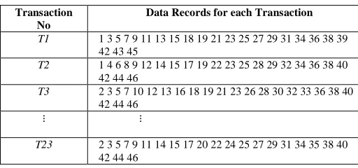
Now, let us consider Table VII in which our dataset file consists of 20 transactional records and each record consists of 23 items in the dataset. So, we have (23*2), i.e., 46 possible values in the dataset and count of each item is calculated by column wise. If Even number appears throughout the column, then the item is shopped otherwise it is not shopped.
Table 7. Transaction and Data Record Details
Transaction No
Data Records for each Transaction
As we mentioned earlier, each item will have two different possibilities i.e., even and odd number for making decision (yes or no). We generating frequent itemsets based on Boolean association rules i.e., there are only two possibilities (Yes/No) for each item.
Figure 12. HP Algorithm: Frequent Itemset Generation
The above Fig. 12 provides a high level illustration of the frequent itemset generation part of HP algorithm for the transaction shown in the table VII.
If we denote the possibilities in un-supervised learning there may be some disadvantages like missing values, incorrect values as the, unsupervised learning refers to the problem of trying to find hidden structure in unlabeled data. Since the examples given to the learner are unlabeled, there is no error or reward signal to evaluate a potential solution. This distinguishes unsupervised learning from supervised learning and reinforcement learning. So, in order to secure the dataset we have to denote it in supervised manner.
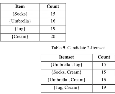
We assume that support threshold is 75% which is equivalent to minimum support of 15. Initially candidate 1-itemset (Table VIII) is generated with support threshold as specified earlier. By using our HP algorithm, we eliminate the weak candidate itemsets (whose support count less than support threshold) before counting the supports by scanning database only once unlike prior algorithm eliminates itemsets after counting the supports.
For example, let us take Min Support Count =15, then we get candidates itemsets as shown in the below.
Table 8. Candidate 1-Itemset
Item Count
{Socks} 15
{Umbrella} 16
{Jug} 19
{Cream} 20
Table 9. Candidate 2-Itemset
Itemset Count
{Umbrella , Jug} 15
{Socks, Cream} 15
{Umbrella , Cream} 16
{Jug, Cream} 19
Table 10. Candidate 3-Itemset
Itemset Count
{Umbrella , Jug, Cream} 15
Here {Socks, Umbrella}, {Socks, Jug} are not generated as candidate 2-Itemsets in Table IX, because their support is not satisfied the support threshold (<15). So, they eliminated automatically. Finally, frequent 3-itemsets are generated as shown in Table X with support count (=15) in single scan.
In the below Fig. 13, we obtain the graph among the maximum size of frequent itemsets generated for different transactional datasets at different intervals of support count, where number of records were differ in each transactional dataset.
Figure 13. Maximum Size of Itemsets generation for Different Support Treshold.
From the above figure we observe that, lowering the support threshold results in more number of maximum size of frequent itemsets and it increases the execution time. Thus we declare maximum size of frequent itemsets increases when there is low support threshold.
VIII.CONCLUSIONSANDFUTUREWORK
In our paper, we have introduced a hybrid parallel algorithm using Radix Trees structures in order to discover association rules in a transaction database. The main aim of our paper is to generate the frequent itemsets which have association among them.
Our algorithm has many features. It scans the database only once, it performs candidate generation in parallel with only few integer exchanges (representing supports computed locally) between processors.
By using [12][2], our HP Algorithm will give best results when compared to previous implementations because the association mining is performed by intersect operation using one key and we proposed a new approach to compute the candidate support by the intersection of Radix Trees.
We currently working on Randomized Search Trees [14] instead of Radix Trees in order to perform intersect operation between two trees to generate association rules.
IX. REFERENCES
[1] Data Mining Concepts and Techniques, Second Edition, Jiawei Han and Micheline Kamber.
[2] C.C´erin, Koskas and Le-Mahec, “Efficient data-structures and parallel algorithms for association rules discovery”. in 3rd International Conference on Parallel Computing Systems (PCS'04), Colima, Mexico, September 2004.
[3] Mohammed J. Zaki. Parallel and distributed association mining: A survey. IEEE Concurrency, 7(4):14–25,/1999.
[4] R.Garg, P.K. MishraK, Exploiting parallelism in Association Rule Mining Algorithms.
[5] Rakesh Agrawal, Tomasz Imielinski, and Arun N.Swami. Mining association rules between sets of items in large databases. In P. Buneman and S. Jajodia, editors, Proceedings of the 1993 ACM SIGMOD Int. Conf. on Management of Data, pages 207–216, Washington, D.C., 26–28 1993.
[6] Mohammed Javeed Zaki, Srinivasan Parthasarathy, and Wei Li. A localized algorithm for parallel association mining. In ACM Symposium on Parallel Algorithms and Architectures, pages 321–330, 1997.
[7] Trie Trees Laboratory Module D.
[8] http://en.wikipedia.org/wiki/selfbalancing-binarysearchtree.
[9] http://en.wikipedia.org/wiki/trie
[10] Viktor Leis, Alfons Kemper, Thomas Neumann, The Adaptive Radix Tree: ARTful Indexing for main-memory databases.
[11] http://en.wikipedia.org/wiki/Radixtree
[12] Michel Koskas. A hierarchical database management algorithm, To appear in the annales du Lamsade, 2004, url: http://www.lamsade.dauphine.fr.
[13] Jeffrey D. Ullman and Jennifer D. Widom. First Course in Database Systems, A, 2/e. Prentice Hall, 2002.
[14] Guy E. Blelloch, Margaret Reid-Miller, Fast Set Operations using Treaps.
[15] Akash Rajak and Mahendra Kumar Gupta, Association Rule Mining: Applications in Various Areas.
[16] Piatetsky-Shapiro, Gregory (1991), Discovery, analysis, and presentation of strong rules, in Piatetsky-Shapiro, Gregory; and Frawley, William J.; eds., Knowledge Discovery in Databases, AAAI/MIT Press, Cambridge, MA.