Ranking by Quality in Spatial Data Using Top k Preference Theory

Volume 3, No. 5, Sept-Oct 2012

International Journal of Advanced Research in Computer Science

RESEARCH PAPER

Available Online at www.ijarcs.info

ISSN No. 0976-5697

Ranking by Quality in Spatial Data Using Top-k Preference Theory

Dwibhashyam Srilalitha*

Student II Year M.Tech (CSE)

Department of Computer Science and Engineering Chaitanya Institute of Science and Technology (CIST)

Madhavi Patnam E.G.Dist. AP India [email protected]

K.Venkata Ramana

Asst. Professor

Department of Computer Science and Engineering Chaitanya Institute of Science and Technology (CIST)

Madhavi Patnam E.G.Dist. AP India [email protected]

M.Vamsi Krishna

Head of the Department

Department of Computer Science and Engineering Chaitanya Institute of Science and Technology (CIST)

Madhavi Patnam E.G.Dist. AP, India [email protected]

Abstract: This spatial preference query ranks objects based on the qualities of features in their spatial neighbourhood. For example, using a real estate agency database of flats for lease, a customer may want to rank the flats with respect to the appropriateness of their location, defined after aggregating the qualities of other features (e.g., restaurants, cafes, hospital, market, etc.) within their spatial neighbourhood. Such a neighbourhood concept can be specified by the user via different functions. It can be an explicit circular region within a given distance from the flat. Another intuitive definition is to consider the whole spatial domain and assign higher weights to the features based on their proximity to the flat. We formally define spatial preference queries and propose appropriate indexing techniques and search algorithms for them. Extensively evaluation of our methods on both real and synthetic data reveals that an optimized branch-and-bound solution is efficient and robust with respect to different parameters

Keywords: Databases, Spatial Data, Spatial databases, querying, analysis of data, ranking data, query processing.

I. INTRODUCTION

All SPATIAL database systems manage large collections of geographic entities, which apart from spatial attributes contain non spatial information (e.g., name, size, type, price, etc.). In this paper, we study an interesting type of preference queries, which select the best spatial location with respect to the quality of facilities in its spatial neighborhood.

Given a set D of interesting objects (e.g. candidate Locations), a top-k spatial preference query retrieves the k objects in D with the highest scores. The score of an object is defined by the quality of features (e.g., facilities or services) in its spatial neighborhood. As a motivating example, consider a real estate agency office that holds a database with available flats for lease. Here “feature” refers to a class of objects in a spatial map such as specific facilities or services. A customer may want to rank the contents of this database with respect to the quality of their locations, quantified by aggregating non spatial characteristics of other features (e.g., restaurants, cafes, hospital, market, etc.) in the spatial neighborhood of the flat (defined by a spatial range around it). Quality may be subjective and query-parametric. For example, a user may define quality with respect to non spatial attributes of restaurants around it (e.g., whether they serve sea food, price range, etc.).

II. SCOREFUNCITON

Given a set of data objects and scored feature objects Query Spatial neighborhood Features of interest (e.g., bars) Returns Ranked set of k best data objects Score of a data object Obtained from feature objects in its spatial neighborhood as per Figure 1.

A. Aggregation of partial scores:

Using sum, max, and min Partial score of a data object for a set of feature objects Defined by the score of a single feature object Highest score, Satisfies the spatial constraint, Spatial constraint, Range, nearest neighbor, and influence.

Figure 2. Range Score Influence Score [1]

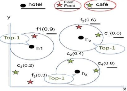
B. Using Max and Min functions in Range and Influence score:

As another example, the user (e.g., a tourist) wishes to find a hotel p that is close to a high-quality restaurant and a high quality cafe. Figure. 2a illustrates the locations of an object data set D (hotels) in white, and two feature data sets: the set F1 (restaurants) in gray, and the set F2 (cafes) in black. The score T(p) of a hotel p is defined in terms of: 1) the maximum quality for each feature in the neighborhood region of p, and 2) the aggregation of those qualities. A simple score instance, called the range score, binds the neighborhood region to a circular region at p with radius e (shown as a circle), and the aggregate function to SUM. For instance, the maximum quality of gray and black points within the circle of p1 are 0.9 and 0.6, respectively, so the score of p1 is T(p1) = 0.9 + 0.6 =

1.5. Similarly, we obtain T(p2) = 1.0 + 0.1 = 1.1 and T(p3) =

0.7 + 0.7 = 1.4. Hence, the hotel p1 is returned as the top result.

For ease of understanding the qualities are normalized to values in [0,1]. In fact, the aggregate function is relevant to the user’s query. The SUM function attempts to balance the overall qualities of all features. The MIN function, the top result becomes the p3, with the score T(p3) = min{0.7 , 0.7} =

0.7. The MAX function, here the top result is p2, with T(p2) =

max{1.0 , 0.1} = 1.0. This is used to optimize the quality in a single feature.

A meaningful score function is the influence score. Figure 2b illustrates the influence score smoothens the effect of e and assigns higher weights to cafes that are closer to the hotel. A hotel p5 and three cafes S1, S2,S3. The circles have their radii

as multiple of e. The score of a café Si is computed by

multiplying its quality with the weight 2-j, where j is the order of the smallest circle containing Si. Let us assume the scoresof

S1, S2, S3 are 0.3/21 = 0.15, 0.9/22 = 0.225 and 1.0/23 = 0.125,

the influence score of p5 is taken as the highest value(0.225)

[1].

III. LITERATURE REVIEW

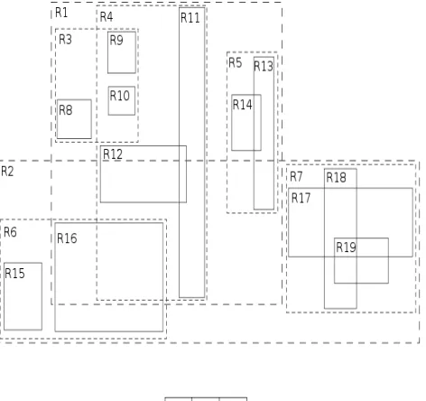
R-trees ar as

was proposed by Antonin Guttman in 1984 and has found significant use in both research and real-world applications. [4] A common real-world usage for an R-tree might be to store spatial objects such as restaurant locations or the polygons that typical maps are made of: streets, buildings, outlines of lakes, coastlines, etc. and then find answers quickly to queries such as "Find all museums within 2 km of my current location", "retrieve all road segments within 2 km of my location" (to display them in a station" (although not taking roads into account).

Figure 3 R-Tree

To group nearby objects and represent them with the the tree; the "R" in R-tree is for rectangle. Since all objects lie within this bounding rectangle, a query that does not intersect the bounding rectangle also cannot intersect any of the contained objects. At the leaf level, each rectangle describes a single object; at higher levels the aggregation of an increasing number of objects. This can also be seen as an increasingly coarse approximation of the data set. As with most trees, the searching algorithms (e.g., bounding boxes to decide whether or not to search inside a sub tree. In this way, most of the nodes in the tree are never read during a search.

Like B-trees, this makes R-trees suitable for large data sets and needed, and the whole tree cannot be kept in main memory.

search, fewer sub trees need to be processed). For example, the original idea for inserting elements to obtain an efficient tree is to always insert into the sub tree that requires least enlargement of its bounding box. Once that page is full, the data is split into two sets that should cover the minimal area each. Most of the research and improvements for R-trees aims at improving the way the tree is built and can be grouped into two objectives: building an efficient tree from scratch (known as bulk-loading) and performing changes on an existing tree (insertion and deletion).

R-trees do not guarantee generally perform well with real-world data. While more of theoretical interest, the (bulk-loaded) the R-tree is also worst-case optimal, but due to the increased complexity, has not received much attention in practical applications so far.

When data is organized in an R-Tree, the

computed using a spatial join. This is beneficial for many algorithms based on the k nearest neighbors.

IV. SPATIALQUERYEVALUATIONONR-TREES

A real estate agency maintains a database that contains information of flats available for rent. A potential customer wishes to view the top 10 flats with the largest sizes and lowest prices. In this case, the score of each flat is expressed by the sum of two qualities: size and price, after normalization to the domain [0, 1] (e.g., 1 means the largest size and the lowest price). In spatial databases, ranking is often associated to nearest neighbor (NN) retrieval. Given a query location, we are interested in retrieving the set of nearest objects to it that qualify a condition (e.g., restaurants). Assuming that the set of interesting objects is indexed by an R-tree, we can apply distance bounds and traverse the index in a branch-and-bound fashion to obtain the answer [5],. Nevertheless, it is not always possible to use multi dimensional indexes for top-k retrieval.

First, such indexes break down in high-dimensional spaces [6], [7]. Second, top-k queries may involve an arbitrary set of user-specified attributes (e.g., size and price) from possible ones (e.g., size, price, distance to the beach, number of bedrooms, floor, etc.) and indexes may not be available for all possible attribute combinations (i.e., they are too expensive to create and maintain). Third, information for different rankings to be combined (i.e., for different attributes) could appear indifferent databases (in a distributed database scenario) and unified indexes may not exist for them. Solutions for top-k queries [3], [8], [9], focus on the efficient merging of object rankings that may arrive from different (distributed) sources.

Their motivation is to minimize the number of accesses to the input rankings until the objects with the top k aggregate scores have been identified. To achieve this, upper and lower bounds for the objects seen so far are maintained while scanning the sorted lists In the following sections, we first review the R-tree, which is the most popular spatial access method and the NN search algorithm of [5] . Then, we survey recent research of feature-based spatial queries.

Figure 4. Spatial Queries on R-Tree [1]

qualities. Hong [10] indexed the data set by a MAX a R-tree and developed an efficient tree traversal algorithm to answer the query. Instead of finding the best k qualities from F in a specified region, our (range score) query considers multiple spatial regions based on the points from the object data set D, and attempts to find out the best k regions (based on scores derived from multiple feature data sets Fc).

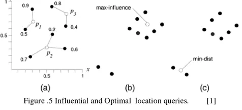
Feature – Based Spatial Queries solved the problem of finding top-k sites (e.g. restaurants) based on their influence on feature points (e.g., residential buildings).[11] As an example, Figure. 5a shows a set of sites (white points), a set of features (black points with weights), such that each line links a feature point to its nearest site. The influence of a site pi is

defined by the sum of weights of feature points having pi as

their closest site. For instance, the score of p1 is 0.9 + 0.5 =

1.4. Similarly, the scores of p2 and p3 are 1.5 and 1.2,

respectively. Hence, p2 is returned as the top-1 influential site.

Related to top-k influential sites query are the optimal location queries studied in [12], [13]. The goal is to find the location in space (not chosen from a specific set of sites) that minimizes an objective function. In Figures. 5b and 5c, feature points and existing sites are shown as black and gray points, respectively. Assume that all feature points have the same quality.

Figure .5 Influential and Optimal location queries. [1]

(a) Top –k influential. (b) Max influence (c) Min distance

The maximum influence optimal location query [12], finds the location (to insert to the existing set of sites) with the maximum influence (as defined in [11]), whereas the minimum distance optimal location query [13], searches for the location that minimizes the average distance from each feature point to its nearest site. The optimal locations for both queries are marked as white points in Figure. 5b, and 5c, respectively. The techniques proposed in [11], [12], [13], are specific to the particular query types described above and cannot be extended for our top-k spatial preference queries. Also, they deal with a single-feature data set whereas our queries consider multiple feature data sets. Recently, novel spatial queries and joins [14], [15], have been proposed for various spatial decision support problems. However, they do not utilize non spatial qualities of facilities to define the score of a location.

V. PROBINGALGORITHMSUSED

A. Simple Probing Algorithm:

The baseline algorithm (Brute Force Algorithm) Simple Probing computes the scores of every object by querying on

feature datasets. This algorithm deals with the collection of information from single reference point.

B. Group Probing Algorithm:

The algorithm Group Probing is a variant of SP that reduces I/O cost by computing scores of objects in the same leaf node concurrently. This algorithm deals with the collection of information from multiple reference point.

In Group Probing the procedures for computing the cth component score for a group of points. Consider a subset V of D for which we want to compute their range score at feature tree Fc. Initially, the procedure is called with N being the root

node of Fc. If e is a non-leaf entry and its mildest from some

point p ∈ V is within the range c, then the procedure is applied recursively on the child node of e, since the sub tree of Fc

rooted ate may contribute to the component score of p. In case e is a leaf entry (i.e., a feature point), the scores of points in V are updated if they are within distance c from e.

Algorithm 1 : Group Range Score Algorithm

Algorithm group_ range (Node N,, Set V,, Value c,, Value e) a. for each entry e ∈N do

b. If N is non-leaf then

c. If ∃p ∈ V, min dist(p, e) ≤ e then d. read the child node N` pointed by e; e. Group_ Range(N`,V, c, e);

f. Else

g. for each p ∈ V such that dist(p, e) ≤ e do

h. Tc (p) := max { Tc (p), w(e)}; [1]

C. Branch and Bound Algorithm:

GP is still expensive as it examines all objects in D and computes their component scores. We now propose an algorithm that can significantly reduce the number of objects to be examined. The key idea is to compute, for non-leaf entries e in the object tree D, an upper bound Z (e) of the score T(p) For any point p in the sub tree of e. If Z (e) * r then we need not access the sub tree of e, thus we can save numerous score computations.

Algorithm 2: Branch and Bound Algorithm Wk: = new min-heap of size k (initially empty); γ : = 0;

Algorithm BB (Node N) a. V: = {e\e ∈ N}; b. If N is non-leaf then c. for c: = 1 to m do

d. compute Tc (e) For all e ∈ V concurrently;

e. remove entries e in V such that T+ (e) ≤ γ; f. sort entries e c V in descending order of? (e); g. for each entry e c V such that Z (e) > v do h. read the child node N pointed by e; i. BB (N);

j. else

k. for c: =1 to m do

l. computeTc (e) For all e ∈ V concurrently;

D. Spatial Data Events:

Spatial database system contains spatial and non-spatial information for road network. Select the spatial location according to client preference. Score is defined by the quality of features and features refer to classes of object in spatial map. Quality of the spatial events may be subjective or query parametric. If the spatial events are subjective then the quality with respective to non-spatial attributes, qualities are normalized to values 0 to 1 and quality values can be obtained from rating providers. The Query-parametric Values are based on the queries. Range score binds neighborhood region to crisp radius and the aggregation of qualities. Influence score smoothens the effect of radius and assign the higher weights.

E. Preferential Queries:

The preference queries involve selecting the best spatial location based on multiple feature data sets on road network. It retrieves k points in a data set with highest score. In the preference queries apply the R-tree indexing feature to data sets with three concepts such as MAX a R-tree to road network, efficient tree traversal algorithm and obtain the quality from rating providers.

F. Ranking of spatial query points:

The two classic ways for ranking objects in spatial data is as follows - 1.Spatial Ranking - It orders according to their distance. 2. Non Spatial Ranking- It orders based on aggregate function. By applying the brute-force approach, compute score of all objects in given set and select the top-k ones. Its very expensive and also complex. We go for Branch bound and optimizing the performance.

G. Top-k Spatial Query:

Top-k spatial preference query retrieves k objects in database with the highest scores. It uses the concept of Branch-and-bound (BB) algorithm and feature join (FJ) algorithm to compute the upper bound score of objects in optimized way. The solution for top-k queries is obtained via merging of object rankings and minimizes the number of access until top-k aggregates reached. An alternate method for top-k query is multi-way spatial join.

The algorithm 2 Branch and Bound derives upper bound scores for non-leaf entries in the object tree and prunes those that cannot lead to better results. This algorithm is responsible for integrating the collected data and performs operations to give the rank for the spatial data.

Adaptations of the proposed algorithms for aggregate functions other than SUM, e.g., the functions MIN and MAX.

VI. ACKNOWLEDGMENT

I thank my Internal guide, and the HOD of our department (who are my co authors) and also Sri Surya Associates who helped me to gather data of houses / flats which are available for let out by allowing me to gather from their database in our area. Also they were interested in our project implementation in real time.

VII. CONCLUSION

Top-k spatial preference queries, which provide a novel type of ranking for spatial objects based on qualities of features in their neighborhood. The neighborhood of an object p is captured by the scoring function:

a. The range score restricts the neighborhood to a crisp region centered at p, whereas

b. The influence score relaxes the neighborhood to the whole space and assigns higher weights to locations closer to p. Search for their relevant objects in the object tree. Here we are using priority based algorithm by selecting the customer who books the flat first by taking the average while calculating Euclidean distance and aggregate obtained when two aggregates or the distances are same with reference to reference points (hospital, school, market, railway station etc) that are located near the flats. Solutions for the top-k spatial preference query based on the influence score can also be developed. In future we will be using this to locate in general the places requested by customers and also the possible way of transportations

VIII. REFERENCES

[1]. Man Lung Yiu, Hua Lu, Member, IEEE, Nikos Mamoulis, and Michail Vaitis, “Ranking Spatial Data by Quality Preference,” Proc. IEEE Transactions on Knowledge and Data Engineering VOL 23, NO. 3, March 2011.

[2]. M.L. Yiu, X. Dai, N. Mamoulis, and M. Vaitis, “Top-k Spatial Preference Queries,” Proc. IEEE Int’l Conf. Data Eng. (ICDE), 2007.

[3]. N. Bruno, L. Gravano, and A. Marian, “Evaluating Top-k Queries over Web-Accessible Databases,” Proc. IEEE Int’l Conf. Data Eng. (ICDE), 2002.

[4]. A. Guttman, “R-Trees: A Dynamic Index Structure for Spatial Searching,” Proc. ACM SIGMOD, 1984.

[5]. G.R. Hjaltason and H. Samet, “Distance Browsing in Spatial Databases,” ACM Trans. Database Systems, vol. 24, no. 2, pp. 265-318, 1999.

[6]. R. Weber, H.-J. Schek, and S. Blott, “A Quantitative Analysis and Performance Study for Similarity-Search Methods in High-Dimensional Spaces,” Proc. Int’l Conf. Very Large Data Bases (VLDB), 1998

[7]. K.S. Beyer, J. Goldstein, R. Ramakrishnan, and U. Shaft, “When is „Nearest Neighbor‟Meaningful?” Proc. Seventh Int‟ l Conf. Database Theory (ICDT), 1999.

[8]. R. Fagin, A. Lotem, and M. Naor, “Optimal Aggregation Algorithms for Middleware,”Proc. Int‟l Symp. Principles of Database Systems (PODS), 2001.

[9]. I.F. Ilyas, W.G. Aref, and A. Elmagarmid, “Supporting Top-k Join Queries inRelational Databases,” Proc. 29th Int‟l Conf. Very Large Data Bases (VLDB), 2003.

Information and Systems, vol. 88-D, no. 11, pp. 2544-2554, 2005.

[11]. T. Xia, D. Zhang, E. Kanoulas, and Y. Du, “On Computing Top-t Most Influential Spatial Sites,” Proc. 31st Int’l Conf. Very Large Data Bases (VLDB), 2005.

[12]. Y. Du, D. Zhang, and T. Xia, “The Optimal-Location Query,” Proc.Int’l Symp. Spatial and Temporal Databases (SSTD), 2005.

[13]. D. Zhang, Y. Du, T. Xia, and Y. Tao, “Progessive Computation of The Min-Dist Optimal-Location Query,” Proc. 32nd Int’l Conf. Very Large Data Bases (VLDB), 2006.

[14]. Y. Chen and J.M. Patel, “Efficient Evaluation of All-Nearest- Neighbor Queries,” Proc. IEEE Int’l Conf. Data Eng. (ICDE), 2007.